The effect of sublattice symmetry breaking on the electronic properties of a doped graphene

Abstract

Motivated by a number of recent experimental studies, we have carried out the microscopic calculation of the quasiparticle self-energy and spectral function in a doped graphene when a symmetry breaking of the sublattices is occurred. Our systematic study is based on the many-body G₀W approach that is established on the random phase approximation and on graphene’s massive Dirac equation continuum model. We report extensive calculations of both the real and imaginary parts of the quasiparticle self-energy in the presence of a gap opening. We also present results for spectral function, renormalized Fermi velocity and band gap renormalization of massive Dirac Fermions over a broad range of electron densities. We further show that the mass generating in graphene washes out the plasmaron peak in spectral weight.

I INTRODUCTION

Graphene is a single atomic layer of crystalline carbon on the honeycomb lattice consists of two interpenetrating triangular sublattices A and B, has opened up a new field for fundamental studies and applications. novoselov1 ; novoselov2 ; novoselov3 ; novoselov4 Peculiar electronic properties of graphene give rise possibility to come over silicon-based electronics limitations. carbon The single-particle energy spectrum in graphene contains two zero-energy at $K^{+}$ and $K^{-}$ points of the Brillouin zone which are called as valleys or Dirac points. Due to the presence of the two carbon atoms per unit cell, the quasiparticle (QP) need to be described by a two component wave function.

The charge carriers in a pristine graphene show linear and isotropic energy dispersion relation and massless chiral behavior for the energy scales up to 1 eV. Recently, graphene has revealed a variety of unusual transport phenomena characteristics of two-dimensional (2D) Dirac Fermions such as an anomalous integer quantum Hall effect at room temperature, a minimum quantum conductivity, Klein tunneling paradox, weak and anti-localization, an absence of Wigner crystallization phase and Shubnikov-deHaas oscillations that exhibit a phase shift of $\pi$ due to Berry’s phase. graphene_rev1 ; graphene_rev2 ; graphene_rev3 ; graphene_rev4 ; graphene_rev5 ; graphene_rev6 ; tomadin One important difference between conventional electron gas and Dirac Fermion particle is that the contribution of exchange and correlation to the chemical potential is an increasing rather than a decreasing function of carrier-density. This property implies that exchange and correlation increase the effectiveness of screening, in contrast to the usual case in which exchange and correlation weakens screening. This unusual property follows from the difference in sublattice pseudospin chirality between the Dirac model’s negative energy valence band states and its conduction band states.

The massless Dirac-like carriers in graphene have almost semi-ballistic transport behavior with small resistance due to the suppression of back-scattering process, and moreover graphene is a good thermal conductor. thermal The mobility of carriers in graphene is quite high morozov1 ; morozov2 ; morozov3 ; morozov4 which is much higher than the electron mobility revealed on the semiconductor hetrostructures. eng1 ; eng2 On the other hand, by measuring the stiffness of materials it is shown that graphene is the strongest material in two-dimension structures. strong1 ; strong2 These properties as well as capability to control of the type and density of charge carriers by gate voltage or the chemical doping dop1 ; dop2 ; dop_lanzara1 ; dop_lanzara2 make graphene an ideal candidate for superior nano-electronic devices operating at high frequencies.

Most electronic applications are based on the presence of a gap between the valence and conduction bands in the conventional semiconductors. The band gap is a measure of the threshold voltage and on-off ratio of the field effect transistors (FETs). FET1 ; FET2 Therefore, for integrating graphene into semiconductor technology, it is crucial to induce a band gap in Dirac points to control the transport of carriers. Consequently, band gap engineering in graphene is a hot topic with fundamental and applied significance. gap In the literature several routes have being proposed and applied to induce and control a gap in graphene. One of them is using quantum confined geometries such as quantum dots and nanoribbons. gap_ribbon1 ; gap_ribbon2 ; gap_ribbon3 ; gap_ribbon4 ; gap_ribbon5 It is shown that the gap values increases by decreasing of nanoribbon width. Another alternative way is spin-orbit coupling whose origin is due to both intrinsic spin-orbit interactions and the Rashba interaction. gap_spin1 ; gap_spin2 ; gap_spin3 ; gap_spin4 Another method to generate a gap in graphene sheets is an inversion symmetry breaking of the sublattices when the number of electrons on A and B atoms are different gapsub1 ; gapsub2 ; gapsub3 ; gapsub4 or Kekulé kekule1 distortion, e.g. graphene on proper substrates dop_lanzara1 ; dop_lanzara2 ; lanzara1 ; lanzara2 ; eva ; gruneis1 ; gruneis2 ; giovannetti or adsorb of some molecules such as water, ammonia ribeiro1 ; ribeiro2 and CrO₃ zanella or an alkali-metal sub-monolayer on graphene sheets.

Recently angle resolved photoemission spectroscopy ( ARPES) experiments on graphene epitaxially grown on SiC and ab initio simulations reported a gap opening in the band structure of graphene placed on proper substrates, and suggested that interactions between the graphene sheet and the substrate leads to symmetry breaking of the A and B sublattices and it consequences to induce a gap in the band structure. Experimenters dop_lanzara1 ; dop_lanzara2 ; lanzara1 ; lanzara2 ; kruczynski observed a gap of 260 meV in band structure of the epitaxial graphene on SiC substrate due to interaction with substrate. In addition, Zhou et al. dop_lanzara1 found a reversible metal-insulator transition and a fine tuning of the carriers from electron to hole by molecular doping in gapped graphene. A Density Functional Theory (DFT) calculation confirmed a substrate induced symmetry breaking. kim . Their results showed a gap in the band spectra of graphene about 200 meV which is in agreement with recent experimental observation. Their calculation determined that there is a 140 meV on-site energy difference between two sublattices. In addition, a band gap is observed in spectra of graphene on Ni(111) substrate gruneis1 ; gruneis2 as well as a gap about of 10 meV in suspended graphene above a graphite substrate eva due to sublattice symmetry breaking mechanism. Moreover, based on the ab initio calculations, it is suggested that boron nitride substrate induced a gap of 53 meV. giovannetti Note that the gap value calculated within DFT is in general underestimating the true band gap value.

In this paper we consider the sublattice symmetry breaking mechanism for a gap opening in a pristine doped graphene sheet and study the impact of gap upon some electronic properties of QPs. To investigate the influence of gap in the many-body properties of QP in graphene we use the random phase approximation (RPA) and the G₀W approximation. It should be noted that a detailed analysis provided a framework for the microscopic evaluation of the QP-QP interaction in the gapless graphene by means of the RPA was carried out by us in Ref. [im1, ] At the beginning, we review briefly the results of the ground state thermodynamic properties that we have already presented elsewhere. alireza Our new results are based on the QP self-energy properties in the presence of a gap opening in the electronic spectrum. From the self-energy we then obtain the QP energies, renormalized Fermi velocity, spectral function which can be compared with ARPES spectra and finally the band gap renormalization of massive Dirac Fermions in doped graphene. We have shown that mass generating in graphene washes out a satellite band in the spectral function in agreement with recent experimental observations. lanzara1

This paper is organized as followed. In Section II we introduce our model Hamiltonian and then review some ground state properties of gapped graphene. In Section III we focus on the properties of imaginary and real parts of self- energy for gapped graphene and then calculate QP spectral function, renormalized Fermi velocity and band gap renormalization. Finally we conclude in Section IV.

II GROUND STATE THERMODYNAMIC PROPERTIES

We consider the sublattice symmetry breaking mechanism in which the densities of particles associated to on-site energy $\mu_{a(b)}$, for A(B) sublattice are different. The electronic structure of graphene can be reasonably good described using a rather simple tight-binding Hamiltonian, leading to analytical solutions for their energy dispersion and related eigenstates. The noninteracting tight binding Hamiltonian for $\pi$ band electrons is determined by gapsub1 ; gapsub2 ; gapsub3 ; gapsub4

$$\hat{H_{0}} = t\sum_{i}(a_{i}^{\dagger}b_{i}+{\rm c.c.})+\mu_{a}\sum_{i}a^{\dagger}_{i}a_{i}+\mu_{b}\sum_{i}b^{\dagger}_{i}b_{i}$$ (1)

$$= t\sum_{i}(a_{i}^{\dagger}b_{i}+{\rm c.c.})+\frac{\mu_{a}-\mu_{b}}{2}\sum_{i}(a^{\dagger}_{i}a_{i}-b^{\dagger}_{i}b_{i})+\frac{\mu_{a}+\mu_{b}}{2}\sum_{i}(a^{\dagger}_{i}a_{i}+b^{\dagger}_{i}b_{i})$$

where the sums run over unit cells, $t\simeq 2.7$ eV denotes the nearest neighbor hopping parameter and $a_{i}(b_{i})$ is Fermi annihilation operator acts on A(B) sublattice. The second term in the noninteracting Hamiltonian breaks the inversion symmetry and causes to a band gap with value of $2\Delta=|\mu_{a}-\mu_{b}|$ at the Dirac points. The last term is a constant and we left it out. The effective Hamiltonian at low excited energies lead to a 2D massive Dirac Hamiltonian, $\mathcal{\hat{H}}_{0}=\hbar v_{\rm F}{\vec{\sigma}}\cdot{\bf k}+\Delta\sigma_{3}$, where $\vec{\sigma}$ are Pauli matrices and $v_{\rm F}=3ta/2\hbar\simeq 10^{6}$ m/s is the Fermi velocity where $a\simeq 1.42$ Å is the carbon-carbon distance in honeycomb lattice. The two eigenvalues of noninteracting Hamiltonian are given by $E_{\bf k}=\pm\sqrt{(\hbar v_{\rm F}k)^{2}+\Delta^{2}}$ for conduction band (+) and valance band (-) which is a fully occupied. In addition, the model Hamiltonian can be used as an approximated model for describing a graphene antidot lattice in the vicinity of a band gap with a small effective mass value antidot , or moreover used as an effective Hamiltonian for the intrinsic spin-orbit interaction in graphene where $\Delta=\Delta_{\rm SO}$ is the strength of the spin-orbit interaction. gap_spin1 ; gap_spin2 ; gap_spin3 ; gap_spin4 If $\mu_{a}=\mu_{b}$ the Hamiltonian reduces to massless Dirac Hamiltonian with two chiral eigenstates having the conical band structures $\varepsilon_{k}=\pm\hbar v_{\rm F}k$.

We consider the long-range Coulomb electron-electron interaction. We left out the intervalley scattering and use the two component Dirac Fermion model. Accordingly, the total interacting Hamiltonian in a continuum model at $K^{+}$ point is expressed as yafis ; Giuliani

$$\hat{H}=\sum_{{\bf k},\sigma}\Psi^{\dagger}_{{\bf k},\sigma}\mathcal{\hat{H}}_{0}\Psi_{{\bf k},\sigma}+\frac{1}{2S}\sum_{{\bf q}\neq 0}V_{q}({\hat{n}}_{\bf q}{\hat{n}}_{-{\bf q}}-{\hat{N}}),$$ (2)

where $\Psi^{\dagger}_{{\bf k},\sigma}=(\psi^{a}_{+,\sigma}({\bf k}),\psi^{b}_{+,\sigma}({\bf k}))$ is two component pseudospinors of the noninteracting Hamiltonian, $S$ is the sample area, ${\hat{N}}$ is the total number operator and $V_{q}=2\pi e^{2}/\epsilon q$ is the bare Coulomb interaction where $\epsilon$ is an average dielectric constant of the surrounding medium. The coupling constant in graphene is $\alpha_{gr}=g_{s}g_{v}e^{2}/\epsilon\hbar v_{\rm F}$ where $g_{s}=g_{v}=2$ being the spin and valley degeneracy, respectively. The coupling constant in graphene depends only on the substrate dielectric constant while in the conventional 2D electron systems is density dependent. The typical value of dimensionless coupling constant is 1 or 2 for graphene supported on a substrate such a SiC or SiO₂.

A central quantity in the many-body techniques is the noninteracting dynamical polarizability function $\chi^{(0)}({\bf q},i\omega,\mu)$ where $\mu$ is the chemical potential. The problem of linear density response is set up by considering a fluid described by the Hamiltonian, $\hat{H}$, which is subject to an external potential. The external potential must be sufficiently weak for low-order perturbation theory to suffice. The induced density change has a linear relation to the external potential through the noninteracting dynamical polarizability function. This function is recently calculated along the imaginary frequency axis and it is given by alireza

$$\chi^{(0)}({\bf q},i\omega,\mu\geq\Delta) = -\frac{g_{s}g_{v}}{2\pi\hbar^{2}v_{\rm F}^{2}}\{\mu-\Delta+\frac{\varepsilon_{q}^{2}}{2}(\frac{\Delta}{{y^{2}}}+\frac{x_{-}^{2}}{2y}\tan^{-1}(\frac{y}{2\Delta}))$$ (3)

$$- \frac{\varepsilon_{q}^{2}}{4y}\Re e\left[x_{-}^{2}(\sin^{-1}\frac{z(\mu)}{x_{+}}-\sin^{-1}\frac{z(\Delta)}{x_{+}})\right]$$

$$+ \frac{\varepsilon_{q}^{2}}{4y}\Re e\left[z(\mu)\sqrt{x_{+}^{2}-z^{2}(\mu)}-z(\Delta)\sqrt{x_{+}^{2}-z^{2}(\Delta)}\right]\},$$

where $x_{\pm}=\sqrt{1\pm 4\Delta^{2}/(\varepsilon_{q}^{2}+\hbar^{2}\omega^{2})}$, $y=\sqrt{\varepsilon_{q}^{2}+\hbar^{2}\omega^{2}}$ and $z(x)=(2x+i\hbar\omega)/\varepsilon_{q}$. The Fermi energy of a 2D massive Dirac Fermion system is given by $E_{\rm F}=\mu=\sqrt{(\hbar v_{\rm F}k_{\rm F})^{2}+\Delta^{2}}$ and the Fermi wavevector is $k_{\rm F}=\sqrt{4\pi n/g_{s}g_{v}}$ where $n$ is the density of carriers. The noninteracting density of states (DOS) is determined by $D(E)=g_{s}g_{v}|E|/2\pi\hbar^{2}v_{\rm F}^{2}\Theta(E^{2}-\Delta^{2})$ which is density dependent at the Fermi surface. It should be noticed that $D(E_{\rm F})$ equals to $m/2\pi\hbar^{2}$ in the conventional 2D electron gas system. Here, $\Theta(x)$ is Heaviside step function.

We now turn to present our first numerical results which are based on the noninteracting polarization function. The static polarization function as a function of wavevector for various gap values is shown in Fig. 1(a). The static polarization function in gapless case is a smooth function whereas a kink at $q=2k_{\rm F}$ occurs for gapped graphene and thus the derivatives of $\chi^{(0)}({\bf q},0,\Delta\neq 0)$ has a singular feature. The singular behavior is the source of several phenomena such as the Friedel oscillations and moreover the Ruderman-Kittel-Kasuya-Yoshida (RKKY) interaction which the later is absent in gapless graphene. In Figs. 1(b) and (c) we have plotted the dynamic polarization function as a function of frequency for wave vectors smaller and larger than $q=2k_{\rm F}$, respectively. $\chi^{(0)}({\bf q},i\omega)$ tends to zero like $\omega^{-1}$ at large frequency region.

The polarization function along the real $\omega$ axis can be obtained by performing analytical continuation of Eq. (3). alireza ; pyatkovskiy1 ; pyatkovskiy2 In Fig. 2 we have presented the real and imaginary parts of the noninteracting polarization function as a function of frequency. Sharp cutoffs in the imaginary part of $\chi^{(0)}({\bf q},\omega)$ are related to the rapid swing in the real part of $\chi^{(0)}({\bf q},\omega)$. These behaviors are in result of the fact that the real and imaginary parts of the polarization function are related through the Kramers-Krönig relations. Importantly, the sign change of the real part from negative to positive shows a sweep across the electron-hole continuum. At very large gap values, the polarization function of massive Dirac Fermions can be reduced to the polarization function (the Lindhard’s function) of conventional two dimensional electron gas systems, as they are determined in Figs. 1 and 2. Consequently, we settle under situation that we can describe a range of band structures from the Dirac’s cone (gapless graphene) to the parabolic (conventional semiconductors) band structure behavior by tuning the gap values from zero to a large value, respectively. We limited our calculations to the intermediate values of of $\Delta$ and we thus expect wide range of the particular properties related to unique behavior of the polarization function.

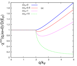
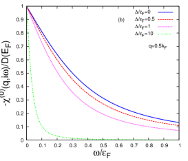
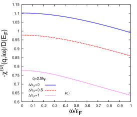
Figure 1: (Color online) (a): The static noninteracting polarization function as a function of $q$ for various $\Delta$. The dimensionless noninteracting dynamic polarization at (b): $q=0.5k_{\rm F}$ and (c): $q=2k_{\rm F}$ as a function of $\omega$ for various $\Delta$.

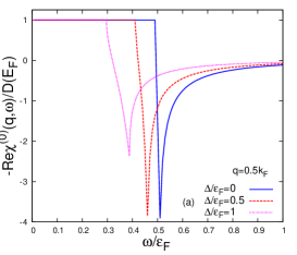
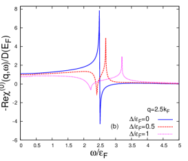
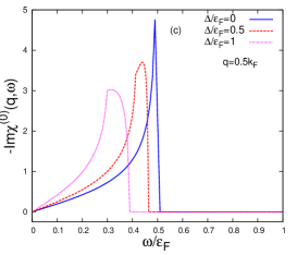
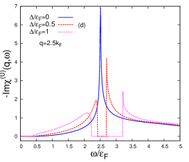
Figure 2: (Color online) The gap dependence of the real and the imaginary part of the noninteracting polarization function as a function of $\omega$ for wavevectors (a), (c) $q=0.5k_{\rm F}$ and (b), (d) $q=2.5k_{\rm F}$

We can calculate the total ground state energy of gapped graphene within RPA. alireza ; yafis The ground-state energies can be calculated using the coupling constant integration technique, which has the contributions $\varepsilon_{tot}=\varepsilon_{kin}+\varepsilon_{\rm xc}$. The kinetic energy per particle is given by $\varepsilon_{kin}=2(E_{\rm F}^{3}-\Delta^{3})/3\varepsilon_{\rm F}^{2}$.

As discussed previously alireza ; yafis we might subtract the vacuum energy contribution from the total energy, $\delta\varepsilon_{tot}=\varepsilon_{tot}(k_{\rm F})-\varepsilon_{tot}(k_{\rm F}=0)$. Due to the number of states in the Brillouin zone must be conserved, we do need a ultraviolet cut-off $k_{c}$, which is approximated by $\pi k_{c}^{2}\simeq(2\pi)^{2}/A_{0}$, where $A_{0}$ is the area of the unit cell. The dimensionless parameter $\Lambda$ is defined as $k_{c}/k_{\rm F}\simeq(g_{s}g_{v}n^{-1}\sqrt{3}/9.09)^{1/2}\times 10^{2}$.

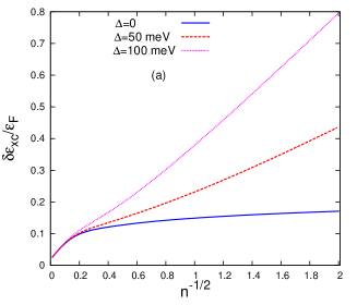
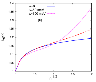
Figure 3: (Color online) (a) Exchange-correlation energy and (b) compressibility as a function of $n^{-1/2}$ ( in units of 10^-6 cm) for various $\Delta$ value.

In Fig. 3, we have shown the exchange- correlation energy in units of $\varepsilon_{\rm F}=\hbar v_{\rm F}k_{\rm F}$, as a function of $n^{-1/2}$ in units of 10^-6 cm for various $\Delta$ value. The exchange energy arises entirely from the antisymmetry of the many-body wave function under exchange of two electrons is positive while the correlation energy, the difference between the ground state energy and the sum of the kinetic energy and the exchange energy is negative. This has important implications on the thermodynamic properties can be calculated from the derivative of the ground state energy with respect to the density. The compressibility can be calculated from its definition, $\kappa^{-1}=n^{2}\partial^{2}(n\delta\varepsilon_{tot})/\partial n^{2}$. Fig. 3(b) shows the ratio between the noninteractiong value, $\kappa_{0}=2/n\varepsilon_{\rm F}$ and the interaction value of compressibility as a function of $n^{-1/2}$. The exchange tends to reduce the compressibility while correlations tends to enhance it. At large $\Delta$, a minimum structure occurs at the inverse of compressibility behavior and we expect that at very large $\Delta$, it starts at $\kappa_{0}$ and reduces by increasing $n^{-1/2}$ behaves like the compressibility of the conversional 2D electron gas.

III THE QP SELF-ENERGY AND THE SPECTRAL FUNCTION

The generation of QPs in an electron liquid leads to two effects. First it induces a decay of a particle losing momentum via inelastic scattering which is determined by the imaginary part of self-energy and second is the renormalization of the dispersion relation of the carriers which is described by the real part of self-energy. $\Re e\Sigma^{\rm ret}({\bf k},\omega)$ is defined as the difference between the measured carrier energy $\hbar\omega$, and the energy of free particle, $\xi_{s{\bf k}}=sE_{{\bf k}}-E_{\rm F}$. To satisfy causality, the real and imaginary parts of self-energy are related by a Hilbert transformation. In this section, we first derive the imaginary and the real part of QP self-energies and then calculate some important quantities such as a renormalized Fermi velocity, a spectral function and a band gap renormalization in the presence of a band gap value. These quantities are related to some important physical properties of both theoretical and practical applications like the band structure of ARPES, the energy dissipation rate of injected carriers and the width of the QP spectral function. kaminski1 ; kaminski2

In the G₀W approximation, the self-energy of gapped graphene is given by ($\beta=1/(k_{B}T)$) fateme :

$$\Sigma_{s}({\bf{k}},i\omega_{n}) = -\frac{1}{\beta}\sum_{s^{\prime}}\int\frac{d^{2}{\bf q}}{(2\pi)^{2}}F^{ss^{\prime}}({\bf k,k+q})$$

$$\times \sum_{m=-\infty}^{+\infty}W({\bf q},i\Omega_{m})G^{(0)}_{s^{\prime}}({\bf k+q},i\omega_{n}+i\Omega_{m}),$$

where $W({\bf q},i\Omega_{m})=V_{q}/\epsilon(q,i\Omega_{m})$ is the dynamical screened effective interaction and $\epsilon(q,i\Omega_{m})=1-V_{q}\chi^{(0)}(q,i\Omega_{m})$ is dynamical dielectric function in RPA. The overlap function for gapped graphene $F^{ss^{\prime}}({\bf k,k+q})$ arises from the graphene band structure is given by alireza

$$F^{ss^{\prime}}({\bf k,k+q})=\frac{1}{2}(1+ss^{\prime}\frac{\hbar^{2}v_{\rm F}^{2}{\bf k}\cdot({\bf k}+{\bf q})+\Delta^{2}}{E_{\bf k}E_{\bf k+q}}).$$ (5)

It should be noted that $F^{s=-s^{\prime}}({\bf q}=0)=0$. However, in gapless graphene, intraband backward scattering should not be allowed, namely $F^{s=s^{\prime}}({\bf q}=-2\textbf{k},\Delta=0)=0$, as well as $F^{s=-s^{\prime}}({\bf q}=0,\Delta=0)=0$. In Eq. (III), $G_{s}^{(0)}({\bf k},i\omega)=1/(i\omega-\xi_{s{\bf k}}/\hbar)$ is the noninteracting Green’s function. Notice that in typical density of carriers in graphene namely $n>10^{12}$cm^-2, the Fermi temperature is about $T_{\rm F}=\varepsilon_{\rm F}/k_{B}>10^{3}$K, and we therefore can eliminate temperature parameter in our calculations. To evaluate the zero-temperature retarded self-energy we perform the line-residue decompositions, $\Sigma^{\rm ret}_{s}({\bf k},\omega)=\Sigma^{\rm line}_{s}({\bf k},\omega)+\Sigma^{\rm res}_{s}({\bf k},\omega)$, where $\Sigma^{\rm line}$ is obtained by performing the analytic continuation before summing over the Matsubara frequencies, and $\Sigma^{\rm res}$ is the correction which must be taken into account in the total self-energy. Giuliani At zero temperature we have

$$\Sigma^{\rm line}_{s}({\bf k},\omega) = -\sum_{s^{\prime}}\int\frac{d^{2}{\bf q}}{(2\pi)^{2}}V_{q}F^{ss^{\prime}}({\bf k,k+q})$$

$$\times \int_{-\infty}^{\infty}\frac{d\Omega}{2\pi}\frac{1}{\epsilon({\bf q},i\Omega)}\frac{1}{\omega+i\Omega-\xi_{s^{\prime}}({\bf k+q})/\hbar},$$

and

$$\Sigma^{\rm res}_{s}({\bf k},\omega) = \sum_{s^{\prime}}\int\frac{d^{2}{\bf q}}{(2\pi)^{2}}\frac{V_{q}}{\epsilon({\bf q},\omega-\xi_{s^{\prime}}({\bf k+q})/\hbar)}F^{ss^{\prime}}({\bf k,k+q})$$ (7)

$$\times [\Theta(\omega-\xi_{s^{\prime}}({\bf k+q})/\hbar)-\Theta(-\xi_{s^{\prime}}({\bf k+q})/\hbar)].$$

The line contribution of the self-energy is purely real. The imaginary part of the self-energy has two contributions where $\Im m\Sigma_{+}^{\rm ret}({\bf{k}},\omega)=\Im m\Sigma_{+,\rm intra}^{\rm res}({\bf{k}},\omega)+\Im m\Sigma_{+,\rm inter}^{\rm res}({\bf{k}},\omega)$, and real part of the self energy can be decomposed as $\Re e\Sigma_{+}^{\rm ret}({\bf{k}},\omega)=\Sigma_{+}^{\rm line}({\bf{k}},\omega)+\Re e\Sigma_{+,\rm inter}^{\rm res}({\bf{k}},\omega)+\Re e\Sigma_{+,\rm intra}^{\rm res}({\bf{k}},\omega)$.

For $\omega>0$ and fixed ${\bf q}$, the RPA decay process represents scattering of an electron from momentum ${\bm{k}}$ and energy $\omega$ to ${\bm{k}}+{\bm{q}}$ and $\xi_{s^{\prime}}({\bm{k}}+{\bm{q}})$, with all energies in Eq. (7) measured from the Fermi energy of doped graphene. Since the Pauli exclusion principle requires that the final state is unoccupied, it must lie in the conduction band, i.e. $s^{\prime}=+1$. Furthermore since the Fermi sea is initially in its ground state, the QP must lower its energy, i.e. $\xi_{s^{\prime}}<\omega$, electrons decay by going down in energy. For $\omega<0$, the self-energy expresses the decay of holes inside the Fermi sea, which scatter to a final state, by exciting the Fermi sea. In this case the final state must be occupied so both band indices are allowed for $s^{\prime}$, and energy conservation requires that holes decay by moving up in energy. Since photoemission measures the properties of holes produced in the Fermi sea by photo ejection, only $\omega<0$ is relevant for this experimental probe.

In what follows, we calculate the intraband and interband contributions of self-energy. We have found the intraband term of residue part of self-energy as following for various values of the frequencies,

$$\Sigma_{+,\rm intra}^{\rm res}({\bf k},\omega>0)=C\int_{\rm max(0,~{}k_{\rm F}-k,~{}k-\beta)}^{k+\beta}dq\int^{\rm min(\hbar\omega+E_{\rm F},~{}\alpha_{+})}_{\rm max(E_{\rm F},~{}\alpha_{-})}dyf_{+}(y,q)$$

$$\Sigma_{+,~{}\rm intra}^{\rm res}({\bf k},\Delta-E_{\rm F}<\hbar\omega<0)=-C\int_{\rm max(0,~{}k-k_{\rm F},~{}\beta-k)}^{k+k_{\rm F}}dq\int^{\rm min(E_{\rm F},~{}\alpha_{+})}_{\rm max(0,~{}\hbar\omega+E_{\rm F},~{}\alpha_{-})}dyf_{+}(y,q)$$

$$\Sigma_{+,\rm intra}^{\rm res}({\bf k},\hbar\omega<-(\Delta+E_{\rm F}))=-C\int_{\rm max(0,~{}k-k_{\rm F})}^{k+k_{\rm F}}dq\int^{\rm min(E_{\rm F},~{}\alpha_{+})}_{\rm max(0,~{}\hbar\omega+E_{\rm F},~{}\alpha_{-})}dyf_{+}(y,q)~{},$$ (8)

where

$$f_{\pm}(y,q)=\frac{\pm(y\pm E_{k})^{2}\mp q^{2}}{\epsilon({\bf q},\omega+E_{\rm F}\mp y)\sqrt{4k^{2}q^{2}-(y^{2}-E_{k}^{2}-q^{2})^{2}}}~{},$$

$C=e^{2}/2\pi\epsilon E_{k}$, $\alpha_{\pm}=\sqrt{\hbar^{2}v^{2}_{\rm F}(k\pm q)^{2}+\Delta^{2}}$ and $\beta=\sqrt{\hbar^{2}\omega^{2}+\hbar^{2}v^{2}k^{2}_{\rm F}+2\hbar\omega E_{\rm F}}$. On the other hand, the interband contribution of residue part of the self energy is determined by

$$\Sigma_{+,\rm inter}^{\rm res}({\bf k},\hbar\omega<-(\Delta+E_{\rm F}))=-C\int_{\rm max(0,~{}k-\beta)}^{k+\beta}dq\int_{\alpha_{-}}^{\rm min(\alpha_{+},-\hbar\omega-E_{\rm F})}dyf_{-}(y,q)~{},$$ (9)

and eventually for the line contribution of self-energy we have

$$\Sigma_{+,\rm intra}^{\rm line}({\bf{k}},\omega) = -\frac{e^{2}}{4\pi^{2}\epsilon}\int_{0}^{k_{c}}dq\int_{0}^{2\pi}d\phi F^{++}({\bf q,q+k},\Delta)\int_{-\infty}^{+\infty}d\Omega\frac{g_{+}(\phi,\Omega,q)}{\epsilon({\bf q},i\Omega)}$$

$$\Sigma_{+,\rm inter}^{\rm line}({\bf{k}},\omega) = -\frac{e^{2}}{4\pi^{2}\epsilon}\int_{0}^{k_{c}}dq\int_{0}^{2\pi}d\phi F^{+-}({\bf q,q+k},\Delta)\int_{-\infty}^{+\infty}d\Omega\frac{g_{-}(\phi,\Omega,q)}{\epsilon({\bf q},i\Omega)}$$ (10)

where

$$g_{\pm}(\phi,\Omega,q)=\frac{\hbar\omega+E_{\rm F}\mp E_{\bf{k+q}}}{(\hbar\omega+E_{\rm F}\mp E_{{\bf k+q}})^{2}+\hbar^{2}\Omega^{2}}$$ (11)

and $\phi$ denotes an angle between ${\bf k}$ and ${\bf q}$. Note that the real part of self-energy is $k_{c}$ dependent.

Now we are in a situation that can calculate some important physical quantities. The QP lifetime or the single-particle relaxation time $\tau$, is obtained by setting the frequency to the on-shell energy in imaginary part of the self-energy, $\tau_{s}^{-1}=\Gamma_{s}({\bf k},{\xi_{s\bf k}}/\hbar)=\frac{2}{\hbar}|\Im m\Sigma_{s}^{\rm ret}({\bf k},\xi_{s\bf k}/\hbar)|$ where $\Gamma_{s}({\bf k},{\xi_{s\bf k}}/\hbar)$ is the quantum level broadening of the momentum eigenstate $|s{\bf k}>$. This quantity is identical with the Fermi’s golden rule expression for the sum of the scattering rate of a QP and quasihole at wavevector ${\bf k}$. Giuliani From Eqs. 8 and 9, one can conclude that total contribution of the imaginary part of the retarded self-energy on the energy shell comes from the intraband term, $\Im m\Sigma_{+}^{\rm ret}({\bf k},\xi_{\bf k}/\hbar)=\Im m\Sigma^{\rm res}_{\rm intra}({\bf k},\xi_{\bf k}/\hbar)$. fateme In the case of gapless graphene, scattering rate is a smooth function because of the absence of both plasmon emission and interband processes. inelastic1 ; inelastic2 However, with generating a gap and increasing the amount of it, plasmon emission cause discontinuities in the scattering time, similar to conventional 2D electron gas. asgari1 ; asgari2 We have thus two mechanisms for scattering of the QPs. The excitation of electron-hole pairs which is dominant process at long wavelength regions and the excitation of plasmon appears in a specific wave vector. As discussed previously fateme , in clean graphene sheets the inelastic mean free path reduces by increasing the gap whereas the mean free path is large enough in the range of the typical gap values 10-130 meV, and thus transport remains in the semi-ballistic regime.

The many-body interactions in graphene as a function of doping can be observed by ARPES which plays as a central role to investigate QP properties such as group velocity and lifetime of carriers on the Fermi surface. ARPES is a useful complementary tool which capable of measuring the constant energy surfaces for all partially occupied states and the fully occupied band structure. The information of band dispersion and the Fermi surface can be elicited from those data measured in ARPES experiments. The relation of the Green’s function to the single-particle excitation spectrum in the interacting fluid is expressed by its spectral function. The spectral function is related to the retarded self-energy by the following expression Giuliani

$$A_{s}({\bf k},\omega)=\frac{\hbar}{\pi}\frac{|\Im m\Sigma_{s}^{\rm ret}({\bf k},\omega)|}{[\hbar\omega-\xi_{s}({\bf k})-\Re e\delta\Sigma_{s}^{\rm ret}({\bf k,\omega})]^{2}+[\Im m\Sigma_{s}^{\rm ret}({\bf k},\omega)]^{2}}$$ (12)

where $\delta\Sigma_{s}^{\rm ret}({\bf k},\omega)=\Sigma_{s}^{\rm ret}({\bf k},\omega)-\Sigma_{s}^{\rm ret}(k_{\rm F},0)$, and then ARPES intensity can be described by $I({\bf k},\omega)=A({\bf k},\omega)n(\omega)$, where $n(\omega)$ is the Fermi-Dirac distribution. The spectral function is the Lorentzian function where $\Re e\Sigma$ specifying the location of the peak of the distribution, and $|\Im m\Sigma|$ is the linewidth. The amplitude of the the Lorentzian function is proportional to $1/|\Im m\Sigma|$. This quantity is the distribution of energies $\hbar\omega$, in the system when a QP with momentum ${\bf k}$, is added or removed from that. For the noninteracting system we get $A^{(0)}({\bf k},\omega)=\delta(\omega-\xi({\bf k})/\hbar)$. The Fermi liquid theory applies only when the spectral function at the Fermi momentum $A^{(0)}(k=k_{\rm F},\omega)$, behaves as a delta function, and has a broadened peak indicating damped QPs at $k\neq k_{\rm F}$.

To progress of the interband single particle excitation and plasmon effects on the $\Im m\Sigma_{s}^{\rm ret}$, we must study the retarded self-energy on the off-shell frequency which is $\omega\neq\xi_{s{\bf k}}/\hbar$. im1 ; im2 This quantity gives the scattering rate of a QP with momentum ${\bf k}$ and kinetic energy $\hbar\omega+E_{\rm F}$. The scattering rate or the linewidth raising from electron-electron interactions is anisotropic and varies significantly via wavevector at a constant energy. The imaginary part of self energy shows the width of the QP spectral function.

In Fig. 4 we have shown the absolute value of the imaginary part of the self energy in unit of $\varepsilon_{\rm F}$ for various gap values. It would be noticed that there is an area of frequency is associated to the gap value, $2\Delta$ in which no QP could enter in. In this case, there is a gap in the $\Im m\Sigma$ between $\xi_{-,k=0}$ and $\xi_{+,k=0}$. We see that $\Im m\Sigma_{+}$ vanishes as $\omega^{2}$ for $\omega$ tends to zero, a universal properties of normal Fermi liquid. Moreover, at large frequency, $\Im m\Sigma_{+}$ tend towards to $\omega$ linearly. Except from the Dirac point, the conduction band $\Im m\Sigma_{+}$ peaks broaden because of the dependence on scattering angle of $\xi({\bf k}+{\bf q})$. For low energy, only intraband single particle excitation contributes to $\Im m\Sigma$ up to $E_{\rm F}$ and then the interband single particle excitation contribution increases sharply about $E_{\rm F}$. The interband contribution increases with increasing the gap values.

To evaluate the scattering rate in interband channel, we have shown $\Im m\Sigma_{inter(intra)}$ as a function of frequency in Fig. 5. The intraband contribution of the imaginary part of self energy associated to scattering rate of QP in the intraband contribution increases with increasing the gap values while the interband contribution reduces, as we physically expected. Moreover, by increasing of the electrons in the conduction band the interband scattering rate reduces whereas the intraband scattering contribution increases. The gap value suppresses the scattering rate at $\omega=-\varepsilon_{\rm F}$.

In Fig. 6 we have plotted the real part of self-energy in unit of $\varepsilon_{\rm F}$ as a function of the energy for various gap values. Notice again that the real part of residue self-energy has a gap which is associated the feature calculated in the imaginary part of self-energy. The line part of self energy is a continues curve and then we have a jump near to the boundary of gap values in the $\Re e\Sigma$ for gapped graphene. A kink around $E_{\rm F}$ is associated to the interband plasmon contribution and it is broaden due to the gap value. This feature affects noticeably in the interacting electron density of states.

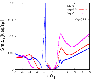
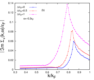
Figure 4: (Color online) The absolute value of the imaginary part of retarded self-energy ( $+$ channel) as a function of (a) $\rm\omega$ and (b) $\rm k$, for the various energy gaps.

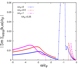
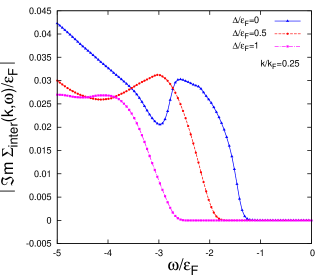
Figure 5: (Color online) (a) The intraband and (b) the interband contributions of the imaginary part of self-energy ( $+$ channel) as a function of $\omega$ for the various energy gaps at $\rm k=0.25k_{\rm F}$.

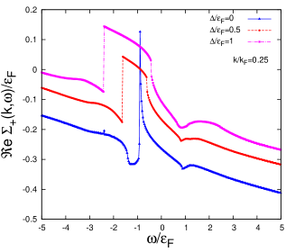
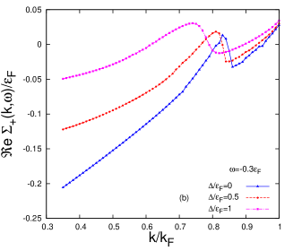
Figure 6: (Color online) The real part of retarded self-energy ( $+$ channel) as a function of (a) $\omega$ and (b) $\rm k$, for the various energy gaps at $\Lambda=100$. The $\Re e\Sigma_{+}$ are measured from the interaction contribution of the chemical potential $\Re e\Sigma_{+}(k_{\rm F},\omega=0)$.

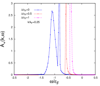
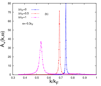
Figure 7: (Color online) The QP spectral function for $+$ channel as a function of $\omega$ (a) and $\rm k$ (b), for the various energy gaps at $\Lambda=100$.

As discussed before im1 ; im2 in a zero temperature and disorder free gapless graphene, the peaks of the spectral function correspond to the nearly solutions of Dyson’s equation in which the quasiparticle excitation energies are obtained by $E=\xi_{+}+\Re e\delta\Sigma_{+}^{\rm ret}$. The intersection of $\Re e\Sigma$ and the lines $E-\xi_{+}$ indicates a satellite long wavelength plasmaron peak related to the electron-plasmon excitation due to the long-range electron-electron Coulomb interaction and the Dyson equation with $\Im m\Sigma=0$ corresponds to a QP peak related to the single particle excitation. Importantly, in the presence of gap values, the plasmaron peak suppressed. In Figs. 7(a) and (b) we have shown the energy distribution curves (EDC) and momentum distribution curves (MDC), respectively. In the presence of gap values, as shown in Fig. 7(a) there is only the single QP peak.

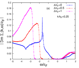
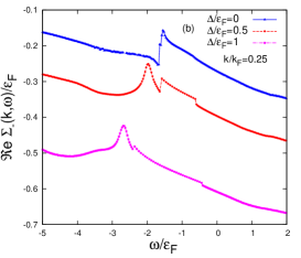
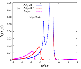
Figure 8: (Color online) The imaginary (a) and real part (b) of the $(-)$ channel of retarded self-energy as a function of $\omega$ for the various energy gaps at $\Lambda=100$. The self-energy are measured from the interaction contribution of the chemical potential $\Re e\Sigma_{-}(k_{\rm F},\omega=0)$. The QP spectral function as a function of $\omega$ (c), for the various energy gaps at $\Lambda=100$.

The valance band self-energy contributions are shown in Fig. 8. There is an area of frequencies is associated to the gap value in which no QP could exist in $\Im m\Sigma_{-}$ exactly the same as the conduction band. The $s=+1$ and $-1$ peaks in $\Im m\Sigma_{s}$ in Figs. 4 and 8 separate at finite $k$ because of chirality factors which emphasize ${\bf k}$ and ${\bf q}$ in nearly parallel directions for conduction band and ${\bf k}$ and ${\bf q}$ in nearly opposite directions for valance band states. Consequently, at finite $\Delta$, the QP peak of $A_{-}(k,\omega)$ which is broaden shifts toward the left in the opposite behavior of $A_{+}(k,\omega)$. These feature have significant effects in the interacting electron density of states.

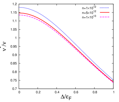
Figure 9: (Color online) The renormalized velocity (+ channel) as a function of the energy gap for various densities at $\alpha_{gr}=1$.

It is essential to note that the satellite band which is theoretically predicted im1 for gapless garphene has not been seen in experiments. There are several reasons that could wash out this feature. For example, the plasmon damping, disorder effects, electron interactions with the buffer layer and importantly the effect of gap at Dirac point.

One of the important information which can be extracted from ARPES spectra is the renormalized Fermi velocity $v^{*}$. A consequence of the interaction is a Fermi velocity renormalization from the backflow of the fluid around a moving particle. The density of states at the Fermi energy is also changed. The QP energy measured from the chemical potential of interacting system $\delta\varepsilon_{sk}^{QP}$, can be calculated by solving self consistently the Dyson equation $\delta\varepsilon_{s{\bf k}}^{QP}=\xi_{s{\bf k}}+\Re e[\delta\Sigma_{s}^{\rm ret}({\bf{\bf k}},\omega)]|_{\omega=\delta\varepsilon_{s{\bf k}}^{QP}/\hbar}$.Giuliani In the isotropic systems the QP energy, depends on the magnitude of ${\bf k}$. Expanding $\delta\varepsilon_{sk}^{QP}$ to first order in $k-k_{\rm F}$ we can write $\delta\varepsilon_{sk}^{QP}\simeq\hbar v^{*}_{s}(k-k_{\rm F})$ which effectively defines the renormalized velocity as $\hbar v^{*}_{s}={d\delta\varepsilon_{sk}^{QP}}/{dk}|_{k=k_{\rm F}}$. From the Dyson equation we can calculated the renormalized Fermi velocity as fateme ; velocity1 ; velocity2

$$\frac{v^{*}_{s}}{v_{s}}=\frac{\varepsilon_{\rm F}E_{\rm F}^{-1}+(\hbar v_{s})^{-1}\partial_{k}\Re e[\delta\Sigma_{s}^{\rm ret}({\bf k},\omega)]|_{\omega=0,k=k_{\rm F}}}{1-\hbar^{-1}\partial_{\omega}\Re e[\delta\Sigma_{s}^{\rm ret}({\bf k},\omega)]|_{\omega=0,k=k_{\rm F}}},$$ (13)

where $v_{s}=sv_{\rm F}$. It is found before fateme ; velocity1 ; velocity2 ; gw1 ; gw2 that electron-electron interaction increases the renormalized Fermi velocity in gapless graphene sheets which this behavior is in contrast to conventional 2DES. asgari1 ; asgari

Fig. 9 shows the renormalized Fermi velocity in unit of the bare Fermi velocity as a function of band gap for various carrier densities. The renormalized Fermi velocity decreasing with increasing the gap value. $v^{*}$ is density independent after $\Delta=0.8\varepsilon_{\rm F}$ which is in good agreement with recent experiment observation. dop_lanzara1 ; dop_lanzara2

Finally we calculated a band gap renormalization (BGR). bgr1 ; bgr2 ; bgr3 ; bgr4 The BGR for conductance band is given by the QP self-energy at the band edge, namely $\rm BGR=\Re e\Sigma_{+}^{\rm ret}({\bf k}=0,\omega=(\Delta-E_{\rm F})/\hbar)$. Fig. 10 shows the BGR for the various gap values as a function of the electron density. The BGR decreases by increasing of the electron density and in the small energy gap values, it is less density dependent respect to large energy gap values. In gapless case, we have obtained a induced band gap or kink due to many-body electron-electron interactions and it tends to a constant with increasing the electron density. im1 ; im2 ; gw1 ; gw2 This feature is in agreement with the results obtained within ab intio DFT calculation. gw1

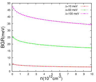
Figure 10: (Color online) The band gap renormalization as a function of electron density for various energy gap at $\alpha_{gr}=1$.

IV SUMMERY AND CONCLUSION

We have revisited the problem of the microscopic calculation of the QP self-energy and many-body effective velocity suppression in a gapped graphene when the conduction band is partially occupied. We have performed a systematic study is based on the many-body G₀W approach that is established upon the random-phase-approximation and on graphene’s massive Dirac equation continuum model. We have carried out extensive calculations of both the real and the imaginary part of the QP self-energy and discussed about the interband and intraband contributions in the scattering process in the presence of gap value. We have also presented results for the effective velocity and for the band gap renormalization over a wide range of coupling strength. Accordingly, we have critically examined the merits of the gap values in dynamical QP properties.

Most feature of mass generating in graphene is the washing out of the plasmaron peak in the spectral weight. Increasing of the gap value makes density independent behavior of the renormalized Fermi velocity. We have shown that the band gap renormalization in gapped graphene decreases by increasing the carrier density at large $\Delta$. This is in contrast with the gapless case in which many body electron-plasmon interactions induce a very small gap in band structure. These distinct features of the massive Dirac’s Fermions are related to mixing of the chiralities and reduce of the interband transitions in graphene sheets.

Acknowledgment

R. A. would like to thank the Scuola Normale Superiore, Pisa, Italy for its hospitality during the period when the final stage of this work was carried out. A. Q. supported by IPM grant.

References

- (1) K. S. Novoselov, A. K. Geim, S. V. Morozov, D. Jiang, Y. Zhang, S. V. Dubonos, I. V. Grigorieva, A. A. Firsov 2004 Science 306 666 .
- (2) K. S. Novoselov, A. K. Geim, S. V. Morozov, D. Jiang, M. I. Katsnelson, I. V. Grigorieva, S. V. Dubonos and A. A. Firsov 2005 Nature 438 197 .
- (3) K. S. Novoselov, D. Jiang, F. Schedin, T. J. Booth, V. V. Khotkevich, S. V. Morozov, and A. K. Geim 2005 Proc. Nat. Acad. Sci. 102 10451 .
- (4) Y. Zhang, Y. Tan, H. L. Stormer, P. Kim 2005 Nature 438 201 .
- (5) P. Avouris, Z. Chen, and V. Perebeinos, 2007 Nature Nanotech. 2 605 .
- (6) A. H. Castro Neto, F. Guinea, N. M. Peres, K. S. Novoselov, and A. K. Geim 2009 Rev. Mod. Phys. 81 109 .
- (7) C. W. Beenakker 2008 Rev. Mod. Phys. 80 1337 .
- (8) A. K. Geim and P. Kim, 2008 Sci. Am. 298 90 .
- (9) A. K. Geim and A. H. MacDonald 2007 Physics Today 60 35 .
- (10) A. K. Geim and K. S. Novoselov 2007 Nature Mater. 6 183 .
- (11) M. I. Katsnelson, 2007 Materials Today 10 20 .
- (12) M. Polini, A. Tomadin, R. Asgari and A. H. MacDonald 2008 Phys. Rev. B 78 115426 .
- (13) A. A. Balandin, S. Ghosh, W. Bao, I. Calizo, D. Teweldebrhan, F. Miao, C. N. Lau 2008 Nano Lett. 8 902 .
- (14) S.V. Morozov, K.S. Novoselov, M.I. Katsnelson, F. Schedin, D.C. Elias, J.A. Jaszczak, A.K. Geim 2008 Phys. Rev. Lett. 100 016602 .
- (15) K. I. Bolotin, K. J. Sikes, J. Hone, H. L. Stormer, and P. Kim 2008 Phys, Rev, Lett. 101 096802 .
- (16) Xu Du, Ivan Skachko, Anthoy Barker and Eva Y. Andrei 2008 Nature Nanotech. 3 491 .
- (17) K.I. Bolotin, K.J. Sikes, Z. Jiang, M. Klima, G. Fudenberg, J. Hone, P. Kim, H.L. Stormer 2008 Solid State Commun. 146 351 .
- (18) K. Eng, R. N. McFarland, and B. E. Kane 2005 Appl. Phys. Lett. 87 052106 .
- (19) E. H. Hwang and S. Das Sarma 2007 Phys. Rev. B 75 073301 .
- (20) C. Lee, X. Wei, J. W. Kysar, J. Hone 2008 Science 321 385 .
- (21) M. Neek-Amal and R. Asgari 2009 arXiv:0903.5035
- (22) T. O. Wehling, K. S. Novoselov, S. V. Morozov, E. E. Vdovin, M. I. Katsnelson, A. K. Geim, A. I. Lichtenstein 2008 Nano Lett. 8 173 .
- (23) I. Gierz, C. Riedl, U. Starke, C. R. Ast, K. Kern 2008 Nano Lett. 8 4603 .
- (24) S. Y. Zhou, D. A. Siegel, A. V. Fedorov, and A. Lanzara 2008 Phys. Rev. Lett. 101 086402 .
- (25) D. A. Siegel, S. Y. Zhou, F. El Gabaly, A. V. Fedorov, A. K. Schmid, and A. Lanzara, 2008 Appl. Phys. Lett. 93 243119 .
- (26) Y. Lin, K. A. Jenkins, A. Valdes-Garcia, J. P. Small, D. B. Farmer, and P. Avouris 2009 Nano Lett. 9 422 .
- (27) J. Kedzierski, P. Hsu, P. Healey, P. W. Wyatt, C. L. Keast, M. Sprinkle, C. Berger, and W. A. de Heer 2008 IEEE Trans. Electron Devices 55 2078 .
- (28) K. Novoselov 2007 Nature Mater. 6 720 .
- (29) Y. W. Son, M. L. Cohen and S. G. Louie 2006 Phys. Rev. Lett. 97 216803 .
- (30) M. Y. Han, B. Ozyilmaz, Y. Zhang and P. Kim 2007 Phys. Rev. Lett. 98 206805 .
- (31) Li Yang, Cheol-Hwan Park, Young-Woo Son, M. L. Cohen, and S. G. Louie 2007 Phys. Rev. Lett. 99 186801 .
- (32) D. Finkenstadt, G. Pennington, and M. J. Mehl 2007 Phys. Rev. B 76 121405(R) .
- (33) Y.-W. Son, M. L. Cohen and S. G. Louie 2006 Nature 444 347 .
- (34) Xue-Feng Wang and T. Chakraborty 2007 Phys. Rev. B 75 033408 .
- (35) Y. Yao, F. Ye, X. L. Qi, S. C. Zhang, and Z. Fang 2007 Phys. Rev. B 75 041401(R) .
- (36) C. L. Kane and E. J. Mele 2005 Phys. Rev. Lett. 95 226801 .
- (37) H. Min, J. E. Hill, N. A. Sinitsyn, B. R. Sahu, L. Kleinman, and A. H. MacDonald 2006 Phys. Rev. B 74 165310 .
- (38) G. W. Semenoff 1984 Phys. Rev. Lett. 53 2449 .
- (39) K. Ziegler, 1996 Phys. Rev. B 53 9653 .
- (40) V. P. Gusynin, S. G. Sharapov, J. P. Carbotte 2007 Int. J. Mod. Phys. B 21 4611 .
- (41) A. Bostowick, T. Ohta, J. L. McCesney, K. V. Emtsev, T. Seyller, K. Horn and E. Rotenberg 2007 New J. Phys. 9 385 .
- (42) C.-Y. Hou, C. Chamon, and C. Mudry 2007 Phys. Rev. Lett. 98 186809 .
- (43) S. Y. Zhou, G. H. Gweon, A. V. Federov, P. N. First, W. A. de Heer, D. H. Lee, F. Guinea, A. H. Castro Neto, and A. Lanzara 2007 Nature Mater. 6 770 .
- (44) S.Y. Zhou, D.A. Siegel, A.V. Fedorov, and A. Lanzara 2008 Physica E 40, 2642 .
- (45) A. Grüneis and D. V. Vyalikh 2008 Phys. Rev. B 77 193401
- (46) A. Grüneis, K. Kummer and D. V. Vyalikh 2009 New J. Phys. 11 073050 .
- (47) G. Li, A. Luican, and E. Y. Andrei 2009 Phys. Rev. Lett. 102 176804 .
- (48) G. Giovannetti, P. A. Khomyako, G. Brocks, P. J. Kelly and J. Van den Brink 2007 Phys. Rev. B 76 073103 .
- (49) M. Polini, R. Asgari, G. Borghi, Y. Barlas, T. Pereg-Barnea, and A. H. MacDonald 2008 Phys. Rev. B 77 081411(R) .
- (50) A. Qaiumzadeh and R. Asgari 2009 Phys. Rev. B 79 075414 .
- (51) R. M. Ribeiro, N. M. R. Peres, J. Coutinho and P. R. Briddon, 2008 Phys. Rev. B 78 075442 .
- (52) Eduardo V. Castro, K. S. Novoselov, S. V. Morozov, N. M. R. Peres, J. M. B. Lopes dos Santos, Johan Nilsson, F. Guinea, A. K. Geim and A. H. Castro Neto 2007 Phys. Rev. Lett. 99 216802 .
- (53) I. Zanella, S. Guerini, S. B. Fagan, J. Mendes Filho and A. G. Souza Filho 2008 Phy. Rev. B 77 073404 .
- (54) M. Mucha-Kruczyński, O. Tsyplyatyev, A. Grishin, E. McCann, Vladimir I. Fal’ko, Aaron Bostwick and Eli Rotenberg 2008 Phys. Rev. B 77 195403 .
- (55) S. Kim, J. Ihm, H. J. Choi, and Y. Son 2008 Phys. Rev. Lett. 100 176802 .
- (56) T. G. Pedersen, A. Jauho, and K. Pedersen 2009 Phy. Rev. B 79 113406 .
- (57) G. F. Giuliani and G. Vignale 2005 Quantum Theory of The Electron Liquid (Cambridge University Press, Cambridge, England) .
- (58) Y. Barlas, T. Pereg-Barnea, M. Polini, R. Asgari and A. H. MacDonald 2007 Phys. Rev. Lett. 98 236601 .
- (59) P. K. Pyatkovskiy, 2009 J. Phys.: Condens. Matter 21 025506 .
- (60) B. Wunsch, T. Stauber, F. Sols and F. Guinea 2006 New J. Phys. 8 318
- (61) A. Kaminski and H. M. Fretwell 2005 New J. Phys. 7 98 .
- (62) A. Damascelli, Z. Hussain, and Z.-X. Shen 2003 Rev. Mod. Phys. 75 473 .
- (63) A. Qaiumzadeh, F. K. Joibari, and R. Asgari 2008 arXv: 0810.4681 .
- (64) E. H. Hwang, BenYu-Kaung Hu, and S. Das Sarma 2007 Phys. Rev. B 76115434 .
- (65) W. Tse, E. H. Hwang, and S. Das Sarma 2008 Appl. Phys. Lett. 93 023128 .
- (66) R. Asgari, B. Davoudi, M. Polini, G. F. Giuliani, M. P. Tosi, and G. Vignale 2005 Phys. Rev. B 71 045323 .
- (67) G. F. Giuliani and J. J. Quinn 1982 Phys. Rev. B 26 4421 .
- (68) E. H. Hwang and S. Das Sarma 2008 Phys. Rev. B 77 081412(R) .
- (69) M. Polini, R. Asgari, Y. Barlas, T. Pereg-Barnea, A. H. MacDonald 2007 Solid State Commun. 143 58 .
- (70) A. Qaiumzadeh, N. Arabchi, R. Asgari 2008 Solid State Commun. 147 172
- (71) Paolo E. Trevisanutto, Christine Giorgetti, Lucia Reining, Massimo Ladisa and Valerio Olevano 2008 Phys. Rev. Lett. 101 226405 .
- (72) C. Park, F. Giustino, C. D. Spataru, M. L. Cohen, and S. G. Louie 2009 Phys. Rev. Lett. 102 076803 .
- (73) R. Asgari and B. Tanatar 2006 Phys. Rev. B 74 075301 .
- (74) Y. Zhang and S. Das Sarma 2005 Phys. Rev. B 72 125303 .
- (75) S. Das Sarma, R. Jalabert, and S. R. Eric Yang 1990 Phys. Rev. B 41 8288 .
- (76) K. F. Berggren and B. E. Sernelius 1984 Phys. Rev. B 29 5575 .
- (77) K. F. Berggren and B. E. Sernelius 1981 Phys. Rev. B 24 1971 .