Ice chemistry in embedded young stellar objects in the Large Magellanic Cloud

Abstract

We present spectroscopic observations of a sample of 15 embedded young stellar objects (YSOs) in the Large Magellanic Cloud (LMC). These observations were obtained with the Spitzer Infrared Spectrograph (IRS) as part of the SAGE-Spec Legacy program. We analyze the two prominent ice bands in the IRS spectral range: the bending mode of CO₂ ice at 15.2 $\mu$m and the ice band between 5 and 7 $\mu$m that includes contributions from the bending mode of water ice at 6 $\mu$m amongst other ice species. The 5$-$7 $\mu$m band is difficult to identify in our LMC sample due to the conspicuous presence of PAH emission superimposed onto the ice spectra. We identify water ice in the spectra of two sources; the spectrum of one of those sources also exhibits the 6.8-$\mu$m ice feature attributed in the literature to ammonium and methanol. We model the CO₂ band in detail, using the combination of laboratory ice profiles available in the literature. We find that a significant fraction ($\gtrsim$ 50%) of CO₂ ice is locked in a water-rich component, consistent with what is observed for Galactic sources. The majority of the sources in the LMC also require a pure-CO₂ contribution to the ice profile, evidence of thermal processing. There is a suggestion that CO₂ production might be enhanced in the LMC, but the size of the available sample precludes firmer conclusions. We place our results in the context of the star formation environment in the LMC.

1 Introduction

The formation of stars in the high-redshift Universe occurred in a metal-poor environment. Much of what we know about the process of star formation is deduced from observations in nearby, Galactic star-forming regions with essentially solar metallicity. However, many of the physical processes that affect star formation and their observational diagnostics are expected to depend on metallicity, for instance cooling and gas-phase and grain surface chemistry. The nearest templates for the detailed study of star formation under metal-poor conditions are the Magellanic Clouds (MCs). The Interstellar Media (ISM) of the Large and Small Magellanic Cloud (LMC and SMC) have significantly lower metallicities ($Z_{\rm LMC}\sim 0.4$ Z_⊙ and $Z_{\rm SMC}\sim 0.2$ Z_⊙), than the solar neighborhood ISM ($Z_{\rm Gal}\sim$ Z_⊙). Only relatively recently are we able to study the details of the star formation process in the MCs (for a review of recent results see Oliveira, 2009).

The star-formation process is a complex interplay of various chemo-physical processes. During the onset of gravitational collapse of a molecular cloud, sufficiently dense cores can only develop if the heat produced during the contraction can be dissipated. The most efficient cooling mechanisms are via radiation through fine-structure lines of carbon and oxygen (e.g., via the emission lines of [C ii] at 158 $\mu$m and [O i] at 63 and 146 $\mu$m), and rotational transitions in abundant molecules such as CO, O₂ and water (Goldsmith & Langer, 1978). These cooling agents all contain at least one heavy atom — H₂ has no permanent dipole moment, and emission through its rotational transitions is very unlikely, making it an inefficient coolant. Besides also contributing to the thermal balance in the molecular cloud, dust grains are crucial in driving cloud chemistry, as dust opacity shields molecules from radiation and grain surfaces enable chemical reactions to occur that would not happen in the gas phase. Surface chemistry is also thought to play an important role in the formation of H₂ (e.g., Williams, 2003) and H₂O (e.g., Hollenbach et al., 2009). Simple theoretical arguments suggest that, even over the range covered by the Milky Way and the MCs, cooling and chemistry rates and timescales are affected by metallicity (Banerji et al., 2009). Not only is it crucial to understand the ISM chemistry at low metallicity, it is also important to investigate the chemical evolution during the star formation process.

In cold molecular clouds, layers of ice form on the surface of dust grains. In particular, when densities increase dramatically during the cold collapse phase, most molecules accrete onto dust grain surfaces. In fact, as water, CO, and also CO₂ are completely frozen out of the gas phase in these environments, ices are substantial reservoirs of the available oxygen and carbon (see review by Bergin & Tafalla, 2007). Even if CO seems to form exclusively in the gas-phase, there is laboratory evidence that water ice is predominantly formed by hydrogenation on icy grains (Ioppolo et al., 2008). Therefore, understanding ice chemistry is crucial to understanding the gas-phase chemistry and the physical conditions within molecular clouds. Water is by far the most abundant ice (typically $10^{-5}-10^{-4}$ with respect to H₂), followed by CO₂ and CO, with a combined abundance of 10$-$30% with respect to water ice (Gibb et al., 2004). Other ice species have also been identified (methanol, ammonia, ammonium, methane and formaldehyde), albeit in much smaller concentrations (van Dishoeck, 2004). While water and CO can be observed from the ground, CO₂ can only be observed from space and its ubiquitous presence in a variety of environments was one of the major discoveries of the Infrared Space Observatory (ISO) (see Ehrenfreund & Fraser, 2003, and references therein).

It is still unknown whether metallicity affects ice chemistry. The most obvious effect of a lower metal content is a reduced availability of carbon and oxygen, the cornerstones of interstellar chemistry. Indeed the CO abundance in the diffuse ISM in the LMC is lower than that measured in Galactic environments (Fukui et al., 2001). In metal-poor clouds, it could be expected that ice abundances are generally depressed (i.e. all ices could be less abundant as a result of lower abundances of C and O), but it is possible that the abundance balance of ice species is also reshaped. The lower dust:gas ratio should make cloud cores more transparent to ambient UV light, possibly exposing ices to more radiative processing, and making complex species more abundant than in the Galaxy.

Interstellar ices have been detected in the envelopes of heavily embedded young stellar objects (YSOs) in the MCs. The first evidence of ices in the envelope of a massive YSO in any extra-galactic environment was a serendipitous discovery by van Loon et al. (2005a). The spectrum of IRAS 05328$-$6827 in the LMC, obtained with the Infrared Spectrometer (IRS, Houck et al., 2004) onboard the Spitzer Space Telescope (Spitzer, Werner et al., 2004) and the Infrared Spectrometer And Array Camera at the Very Large Telescope (ISAAC/VLT), shows clear absorption signatures of water ice at 3.1 $\mu$m and CO₂ ice at 15.2 $\mu$m. Oliveira et al. (2006) and Shimonishi et al. (2008) identified more embedded YSOs with ice signatures in the LMC. Three embedded YSOs have been recently identified in the SMC (van Loon et al., 2008). There is a suggestion that the stronger UV radiation field (Welty et al., 2006) and/or higher dust temperature (Aguirre et al., 2003) could be responsible for a higher CO₂-to-water column density ratio observed towards a few YSOs in the LMC when compared to Galactic YSOs (van Loon et al., 2005a; Shimonishi et al., 2008). These studies are however hampered by small sample size and limited spectral resolution and thus not yet conclusive.

CO₂ ice is found to be abundant and ubiquitous in a variety of molecular environments in the Galaxy, from quiescent clouds (Whittet et al., 2007) to the envelopes of high- and low-luminosity YSOs (Gerakines et al., 1999; Pontoppidan et al., 2008). This molecule is generally believed to form exclusively via surface reactions, even though its formation mechanism is not fully understood (for a recent discussion of this issue see Pontoppidan et al., 2008). The most prominent CO₂ solid state features are the 4.3-$\mu$m stretching and 15.2-$\mu$m bending modes (e.g., Ehrenfreund et al., 1997). Comparisons of observed 15.2-$\mu$m profiles with laboratory spectra suggest that CO₂ ices are dominated by components that are either water- or CO-rich, rather than pure CO₂ (Gerakines et al., 1999; Pontoppidan et al., 2008; Whittet et al., 2009). For some YSOs, narrow substructure in the observed profiles provides evidence of thermal processing (e.g., Gerakines et al., 1999; White et al., 2009). Therefore the CO₂ ice profile is a sensitive probe of its molecular environment.

Another ice band in the IRS range (5$-$7 $\mu$m) is less well understood, with contributions not only from water ice at 6 $\mu$m but also ammonia (NH₃), methanol (CH₃OH), formic acid (HCOOH) and formaldehyde (CH₂O) ices (Boogert et al., 2008). This superposition of multiple ice components is possibly responsible for the discrepancy between the column densities determined from the 3-$\mu$m (O$-$H stretching mode) and the 6-$\mu$m (O$-$H bending mode) water ice features, with the 6-$\mu$m column density systematically higher (Gibb et al., 2004; Boogert et al., 2008). There is an ice feature at 6.8 $\mu$m attributed to ammonium (NH${}_{4}^{+}$) (Boogert et al., 2008). This band also falls in a wavelength range strongly affected by emission features generally attributed to polycyclic aromatic hydrocarbon (PAH) molecules. The libration mode of water ice is a very broad feature that peaks at 13 $\mu$m and extends between 10$-$30 $\mu$m; in practice this feature is very difficult to isolate both because of its width and the fact that it is hard to disentangle from the more prominent silicate dust features.

In a series of papers we will investigate ice chemistry in the envelopes of massive embedded YSOs in the low metallicity environment of the MCs. The Spitzer Legacy survey of the LMC (SAGE, Meixner et al., 2006) identified large numbers of YSO candidates for the first time in any extra-galactic environment (Whitney et al., 2008). The follow-up Legacy program with the Spitzer-IRS includes a variety of point and extended sources among which YSOs feature prominently (SAGE-Spec, Kemper et al., 2009). We selected the LMC sample described here from both the SAGE-Spec program and the Spitzer archive, as those objects that have spectral energy distributions (SEDs) consistent with early embedded YSOs and exhibiting in their spectrum the absorption feature associated with CO₂ ice, the most prominent ice band in the Spitzer-IRS spectral range.

In this paper we present the first detailed analysis of CO₂ ice profiles for massive YSOs in the LMC. The paper is organized as follows. First we introduce the sample and discuss the issues of continuum determination and constraining the PAH spectrum. We then describe the observed CO₂ profiles in terms of laboratory components and measure column densities. We also investigate features in the 5$-$7 $\mu$m range. Finally we interpret our results in terms of possible effects of low metallicity.

2 Observations and data reduction

The Spitzer-IRS spectra of our target sample were obtained mostly as part of the Spitzer SAGE-Spec Legacy program (PID: 40159). For three targets, IRS spectra were recovered from the archive (PIDs: 3591, 3505). Kemper et al. (2009) describe in detail the original target selection, observing strategy, and data reduction for the SAGE-Spec program; we provide here only a brief summary.

The IRS observations of the point sources in SAGE-Spec were performed in staring mode, using the Short-Low and Long-Low modules (SL and LL respectively). The 8- and 24-$\mu$m fluxes were used to set exposure times, aiming at signal-to-noise ratios of $\sim$ 60 in SL and $\sim$ 30 in LL. Archival spectra mentioned previously were also obtained in staring mode with SL and LL.

The spectra were reduced following standard reduction techniques. Flatfielded images from the standard Spitzer reduction pipeline were background subtracted and cleaned of “rogue” pixels and artifacts. Spectra were extracted individually for each data collection event (DCE) and co-added to produce one spectrum per nod position. The nods were combined to produce a single spectrum per order, rejecting “spikes” that appear in only one of the nod positions. Finally, the spectra of all the segments were combined including the two bonus orders, that are useful in correcting for discontinuities between the orders. Archival spectra of LMC objects were re-reduced by the SAGE-Spec team to the same uniform standard as the SAGE-Spec sources.

When comparing spectra obtained with different instruments, and of objects at different distances, it is important to consider potential differences in the physical scales that are sampled. The Spitzer IRS slits are $3.6^{\prime\prime}$ and $10.5^{\prime\prime}$ wide, respectively for the SL and LL modes. In the cross-dispersion direction the typical 2-pixel scales sampled are $3.6^{\prime\prime}$ and $10.2^{\prime\prime}$, respectively. At the distance of the LMC ($d\approx$ 50 kpc), these approximately square regions on the sky correspond to 0.9 $\times$ 0.9 pc² and 2.5 $\times$ 2.5 pc² at 6 $-$ 7 and 15 $\mu$m, respectively.

By comparison, the ISO SWS apertures are $14^{\prime\prime}\times 20^{\prime\prime}$ around 3 and 6 $-$ 7 $\mu$m, and $14^{\prime\prime}\times 27^{\prime\prime}$ around 15 $\mu$m. Observations obtained with these modules of massive-star forming regions in the Galaxy at typical distances of $\sim$ 1.5 kpc sample physical scales of $0.10\times 0.15$ pc² and $0.10\times 0.20$ pc² at 6$-$ 7 and 15 $\mu$m, respectively. Hence these SWS observations would sample scales roughly ten times smaller in typical Galactic regions than the Spitzer observations in the LMC. Observations obtained with Spitzer of low-mass YSOs in nearby complexes at typical distances $d\approx$ 150$-$ 350 pc sample even finer scales, by a factor $\sim$ 200 compared to observations in the LMC.

3 The massive YSO sample

This study focuses on the least evolved, most embedded massive YSOs in the LMC. Embedded YSOs can be selected based on their mid-IR colors. However, the colors and even broad-band SEDs of YSOs are in some instances similar to those of evolved objects like planetary nebulae and post-AGB stars. Whitney et al. (2008) discuss in detail the YSO selection criteria using Spitzer data and contamination by evolved stars. One of the main goals of the SAGE-Spec program is to use spectra to clarify the boundaries between different classes of objects in the color-color and color-magnitude space. For this study we have selected only objects whose nature is spectroscopically unambiguous, which also means that these objects are the most embedded and luminous.

We initially identified YSO candidates based on their very red continuum over the 5$-$38 $\mu$m range. Then we narrowed the sample to include only those objects that showed an indication of the CO₂ ice feature at 15.2 $\mu$m. CO₂ in the gas phase has been detected towards many AGB stars (e.g., Justtanont et al., 1998); CO₂ ice however is only observed in YSO envelopes and quiescent molecular clouds (Section 4.3) — water ice is also observed in the envelopes of evolved stars (e.g., Dijkstra et al., 2003). Therefore the shape of the SED and the CO₂ ice feature unambiguously identify these objects as embedded YSOs. We did not make use of the 5$-$7 $\mu$m ice complex for sample selection, because this wavelength range is dominated by PAH emission in our YSO sample (see below).

The final sample then includes 15 objects, 10 of which were classified as “high-probability YSOs” based only on their IRAC colors (Whitney et al., 2008). Tables 1 and Ice chemistry in embedded young stellar objects in the Large Magellanic Cloud provide the positions and observed fluxes for the YSOs. Even if some objects are known IRAS or MSX sources, many objects had not been classified or studied prior to the Spitzer surveys. Van Loon et al. (2005a) analyzed the IRS and ground-based L-band spectra of IRAS 05328$-$6827, which show ice signatures; we re-analyzed here its IRS spectrum. Shimonishi et al. (2008) obtained low-resolution AKARI near-IR spectra (3$-$5 $\mu$m, Murakami et al., 2007) of three of the sources, which also showed ice features. Van Loon et al. (2005b) tentatively identified IRAS 05246$-$7137 as an AGB or post-AGB object. More recently, Whitney et al. (2008) classified this source as a YSO based on its IRAC colors. The object’s IRS spectrum (showing strong silicate absorption, weak PAH emission, and a tentative ice detection) and IR luminosity support the YSO classification. MSX LMC 464 was tentatively identified as a possible H ii region (Kastner et al., 2008) based on 2MASS and MSX colors. Van Loon et al. (2009) describe the Spitzer MIPS-SED spectra (Rieke et al., 2004) of IRAS 05328$-$6827, MSX LMC 1786, and IRAS 05246$-$7137; they all show a cold dust continuum between 53$-$92 $\mu$m consistent with a YSO status.

4 Analysis of the IRS spectra and ice absorption features

Figure 1 shows the spectra of the 15 objects analyzed in this work, covering the whole IRS range. The insets show the spectral regions associated with the ice bands, CO₂ at 15.2 $\mu$m and the 5$-$7 $\mu$m complex. Objects are displayed in decreasing flux intensity at 5.8 $\mu$m. Many objects show broad absorption at 10 $\mu$m (and occasionally 18 $\mu$m) attributed to silicate dust grains; one object (IRAS 05240$-$6809) shows silicate emission. PAH emission is also present in many objects in our sample: the prominent 6.2- and 11.3-$\mu$m PAH features are easily identified in at least two thirds of the spectra. Figure 1 also shows that there are a variety of strength and profile shapes associated with the CO₂ ice and that few objects exhibit clear ice absorption at 6 $\mu$m. In the next sections we will analyze these features in more detail, starting with the issue of continuum determination.

4.1 YSO properties: SED fitting

We have fitted the observed SEDs of the LMC YSOs using the on-line fitting tool developed by Robitaille et al. (2007). This tool relies on a database of 20,000 pre-calculated models that are compared to the observed SEDs, and the best fit is selected using a $\chi^{2}$ minimization technique. Robitaille et al. (2006, 2007) explain these tools in more detail, and Chen et al. (2009) give examples of their use. A typical YSO model includes a central stellar photosphere, a flared accretion disk, and a rotationally flattened infalling envelope with bipolar cavities, characterized by a total of 14 parameters. The balance of the different model components determines the object’s evolutionary status.

To constrain the observed SEDs we made use of the IRS spectrum discussed here as well as all the photometric data available for each object (Tables 1 & Ice chemistry in embedded young stellar objects in the Large Magellanic Cloud). The SEDs of 10 objects are described by Whitney et al. (2008); for the remaining objects the results of the SED fits will be discussed in detail by Chen et al. (in preparation). The objects in the sample have estimated YSO luminosities in the range $\sim$ 5 $-$ 50 $\times$ 10³ L_⊙ and masses between $\sim$ 10 and 25 M_⊙. Taking into account their observed luminosity, the objects in our sample are the LMC counterparts of the luminous Galactic YSOs such as those studied by Gerakines et al. (1999) and Gibb et al. (2004) with ISO. In terms of evolutionary stages the YSOs are all in Stage I, i.e they are still deeply embedded in their envelopes, as expected from the presence of ice absorption features. The Stage I classification is equivalent to the Class I as defined by Lada (1987), but instead of relying on the spectral index of the SED, it is based on modelled SED quantities, in this case the accretion rate of the envelope normalized to the stellar mass, Ṁ_env/$M_{\star}$ $>$ 10^-6 yr^-1 (Robitaille et al., 2006).

4.2 Dust continuum, PAH emission and silicate features

The mid-IR spectra of embedded YSOs exhibit a wealth of solid-state and gas features super-imposed on a dust continuum: silicate absorption/emission features at 10 and 18 $\mu$m, PAH emission features from 5 to 19 $\mu$m, molecular hydrogen and forbidden line emission across 5 $-$ 35 $\mu$m and finally the ice signatures we are interested in here. In our sample, 11 out of 15 objects show prominent PAH emission (look for the conspicuous 11.3-$\mu$m feature in Figure 1). As we want to measure ice optical depth, we need both to determine the continuum level and account for any emission or absorption features that fall in the desired spectral ranges. We fitted continua between 5 and 20 $\mu$m, focusing on obtaining good continuum determinations around 5 $-$ 7 and 15 $\mu$m.

Determining a global IR continuum for YSOs is not trivial. This is because the lines and bands listed above merge together, meaning that few true continuum points exist across the spectrum. As a consequence continuum fits rarely offer unique solutions. The CO₂ ice band at 15.2 $\mu$m is relatively narrow and falls in the region between the 11.3$-$12.7 $\mu$m and 17-$\mu$m PAH complexes and between the silicate absorption bands. Therefore, it is possible and practical to use a local continuum determination, for instance a low-order polynomial fitted to the local pseudo-continuum in the neighborhood of the ice feature.

This is not the case for the 5$-$7 $\mu$m ice band. First, there is prominent PAH emission in this region, namely the 6.3-$\mu$m feature and the 7.7-$\mu$m complex, as well as unresolved H₂ emission at 5.51 (S7), 6.11 (S6), and 6.91 $\mu$m (S5). Spoon et al. (2002) show that relatively weak water ice signatures at 6 $\mu$m are difficult to separate from the PAH emission contribution. Secondly, this range falls at the edge of the IRS spectrum, where the spectra are noisier. This means that it is very difficult if not impossible to find bona-fide continuum points to anchor a local pseudo-continuum determination.

PAHFIT (Smith et al., 2007) provides a convenient way of constraining the dust continuum and extinction as well as accounting for PAH and gas emission. The dust continuum is modelled with up to eight thermal dust components represented by modified blackbodies of a range of temperatures; dust extinction is produced by adopting extinction profiles similar to those of Milky Way dust. PAH emission features are represented by individual and blended Drude profiles — depending on whether PAH complexes are resolved into their multiple components — with fixed widths and central wavelengths. Molecular and atomic emission lines (e.g., H₂ pure rotational lines, forbidden line emission from [S iii], [Ne ii], and [Ne iii] etc) are modelled as Gaussian profiles; their widths and central wavelengths are allowed to change to account for the fact that these lines are not resolved in the IRS low-resolution spectra. To help PAHFIT constrain the continuum we added the IRAC 3.6- and 4.5-$\mu$m photometric points to the IRS range. The very broad water libration mode at 13 $\mu$m is treated as a component of the continuum in this approach. Once all the PAHFIT components are accounted for, we are left only with the ice contributions.

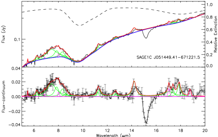
Figure 2: Fits to YSO spectra using PAHFIT: spectra with all fitted components (upper panels) and continuum-subtracted spectra (lower panels). The total fit is shown (red) as well as the individual components of the fit: dust continuum (blue), PAH emission (green) and atomic and molecular emission lines (magenta) — in some cases there is a very small contribution from starlight. Also shown is the silicate dust relative extinction as fitted by PAHFIT (right-hand axis).

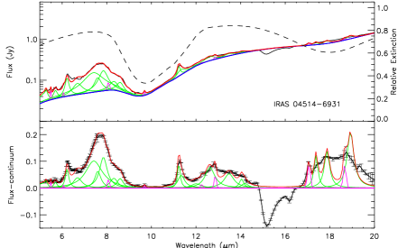
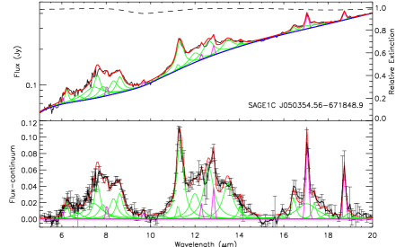
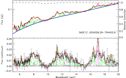
Figure 2: Continued.

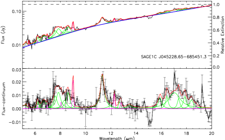
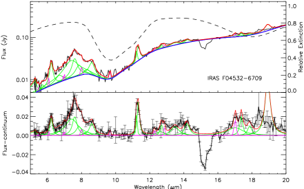
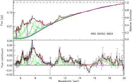
Figure 2: Continued.

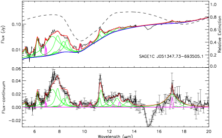
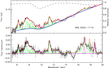
Figure 2: Continued.

Figure 2 shows fits to the 11 YSOs in the sample with PAH emission, using PAHFIT. Total fits are shown, as well as color-coded individual contributions of dust continuum, PAH emission and molecular and atomic line emission. For each object we show their spectrum and the continuum-subtracted spectrum to highlight the PAH contribution. We found that PAHFIT fits the spectra well from 5$-$17 $\mu$m. PAH emission is unequivocal in Figure 2. In terms of general appearance, the continuum-subtracted spectra of objects like MSX LMC 464, SAGE1C J050354.56$-$671848.9, and IRAS 05452$-$6924 are reminiscent of the spectral components between 5 and 14 $\mu$m attributed to neutral PAHs, PAH clusters, and PAH cations (Tielens, 2008).

At longer wavelengths, we find that PAHFIT has some trouble fitting the red side of the 17-$\mu$m PAH complex that also includes H₂ emission at 17.0 $\mu$m (examples are IRAS 04514$-$6931 and IRAS F04532$-$6709 in Figure 2). In particular at about 18 $\mu$m there seems to be more emission than can be produced by PAHFIT: there are no known PAH emission features between 17.9 and 18.9 $\mu$m. It is also not due to spurious “features” related to diffuse gas in the LMC (i.e. [S iii] at 18.7 $\mu$m, as mentioned by Buchanan et al. 2006). The 17-$\mu$m complex is not as well studied as other, shorter-wavelength PAH features. Even though identified with ISO-SWS, it was only Spitzer-IRS that allowed a more detailed analysis of this complex (see Tielens, 2008, for a review). It is described as a broad plateau that can extend from 16 to 19 $\mu$m, but observations show a varied substructure. Van Kerckhoven et al. (2000) and Peeters et al. (2004) have used large molecule databases to show that a huge range of merged profile structures can be achieved by combining individual PAH emission contributions. Thus it is not surprising that the fits are not perfect in this region. None of this affects the continuum underlying the ice bands.

We note that a detailed analysis of PAH emission is beyond the scope of this paper, but we verified that PAHFIT is an adequate tool to use in the context of a YSO study. While the spectral contributions underlying the CO₂ ice feature are well constrained, that is not the case for the 5$-$7 $\mu$m ice complex. Even using PAHFIT to account for emission features, it is very difficult to isolate this ice band: the only objects for which this was possible have no detectable PAH emission (see below).

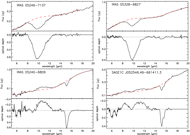
Figure 3: Continuum fits to YSO spectra without PAH emission. For each object the total continuum fit is shown (red dashed line, low-degree polynomial) as well as the optical depth spectra. The two objects at the top have strong silicate absorption and weak CO₂ ice; the two objects at the bottom exhibit either a self-absorbed or emission silicate feature and strong CO₂ ice.

The four remaining objects do not show obvious PAH emission in their spectrum; we thus adopt the traditional approach of fitting a low-order polynomial to the continuum. Continuum points are selected to avoid the ice bands at 5 $-$ 7 and 15.2 $\mu$m and the silicate feature at 10 $\mu$m. The 18-$\mu$m silicate feature and the water libration mode are very broad, and we do not try to extract them from the spectra; instead we treat them as contributing to the local “pseudo-continuum”. Figure 3 shows the continuum fits for these objects. The two objects at the top (IRAS 05246$-$7137 and IRAS 05328$-$6827) show strong silicate in absorption and weak CO₂ ice absorption. SAGE1C J052546.49$-$661411.3 and IRAS 05240$-$6809 show silicate emission and self-absorption respectively, even though the nature of the silicates is difficult to constrain without a detailed study. In general the silicate optical depth is not well constrained as the shape of the continuum underlying it is somewhat uncertain. Both these objects show ice absorption at 15.2 and 6 $\mu$m. IRAS 05240$-$6809 also shows H₂ emission at 5.51, 6.91, and 9.66 $\mu$m. These two apparently PAH-free objects are the only YSOs for which we were able to successfully isolate the 5 $-$ 7 $\mu$m ice band.

For the 11 PAH-rich YSOs we use the PAHFIT output to extract the optical depth of the ice features, for the remaining objects we use the spectrum after subtracting a polynomial continuum. We compared the optical depth spectra obtained when using the PAHFIT and the polynomial continua, for these four objects. This allowed us to constrain how the choice of continuum affects the measured column densities for the ice features (Section 4.3.3)

4.3 CO₂ ice at 15.2 $\mu$m

It has been shown in laboratory experiments that the CO₂ ice profile at 15.2 $\mu$m is a sensitive probe of the environment in which the ice resides, both in terms of physical conditions like temperature (it traces strong heating, Ehrenfreund et al., 1998; Gerakines et al., 1999; White et al., 2009) and also in terms of molecular environment (it can indirectly pinpoint other molecules in the ice matrix, Ehrenfreund et al., 1997) as is discussed in the next section. On one hand this makes CO₂ an interesting ice species to study, but on the other it implies that laboratory studies of this solid are very complex as the whole molecular system needs to be considered, not just CO₂ ice in isolation. Realistic astrophysical environments are also impossible to replicate. Thus we cannot model the CO₂ profiles directly using experiments. The next best thing is a phenomenological approach that attempts to model the observed profiles as a combination of “components” that have been well studied in the laboratory.

CO₂ does not form in any sizable abundance in the gas phase in the diffuse interstellar medium or molecular clouds (e.g., Herbst & Leung, 1986), but it is not yet fully understood which of a number of possible grain-surface reactions is responsible for the abundance and ubiquity of CO₂ ices (for a recent discussion on CO₂ formation mechanisms see Pontoppidan et al., 2008). It was initially thought that this molecule would form during strong UV photolysis of mixed ices containing H₂O and CO (e.g., D’Hendecourt et al., 1986), conditions easily found in the envelopes of luminous embedded YSOs. However, observations of abundant CO₂ also in the quiescent ISM (Whittet et al., 2007, 2009) indicate that additional radiative processing, besides that provided by cosmic-ray induced photons and ambient radiation field photons, is not required for CO₂ formation.

H₂O ice is the most abundant ice species, followed by CO and CO₂ (Gibb et al., 2004). These distinct ice species are often observed in the same sightline and are present on the same grain mantles possibly in a layered, “onion”-like structure. In particular, two independent components have been identified on icy mantles: H₂O-dominated and CO-dominated components, also referred to as polar and apolar components, respectively (Tielens et al., 1991; Ehrenfreund & Fraser, 2003). A possible scenario is that H₂O ice (with traces of CO, NH₃, and CH₄) forms easily and widely in molecular clouds, as it requires relatively low gas density and only moderately low temperature. At higher densities grains accrete mainly apolar molecules like CO (and IR inactive molecules like O₂ and N₂, see below); this rapid freezeout creates a mantle of almost pure CO on top of a water-rich layer (Tielens et al., 1991; Ehrenfreund et al., 1997).

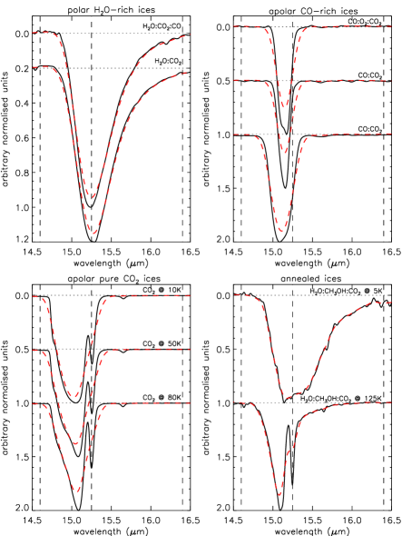
Figure 4: Representative laboratory ice profiles for the different types of mixtures considered here: H₂O-rich, CO-rich, pure-CO₂ and annealed ices. The profiles used are listed in Table 3. For the CO-rich ices the following compositions are shown: CO:O₂:CO₂ = 100:50:16, CO:CO₂ = 100:16 and CO:CO₂ = 100:70. Dashed (red) lines are the laboratory profiles smoothed to match the resolution of the Spitzer IRS LL mode (see text). The double-peaked structure of the pure-CO₂ and annealed ices is smoothed out to such an extent that it is no longer clearly identifiable. The vertical lines delimit the red and blue wing of the profile (see text).

Laboratory experiments show that 15.2-$\mu$m CO₂ profiles in ice matrices dominated by either H₂O or CO have very distinct properties (e.g., Ehrenfreund et al., 1997, see also Figure 4). The comparison of laboratory and astronomical CO₂ ice profiles shows that the latter are well represented by a combination of polar (H₂O-dominated) and apolar (CO-dominated) components (Gerakines et al., 1999; Whittet et al., 2007; Pontoppidan et al., 2008; White et al., 2009; Whittet et al., 2009). The polar component usually dominates, accounting for a large fraction of the total CO₂ column density (Gerakines et al., 1999; Pontoppidan et al., 2008; Whittet et al., 2009). Thus, even though doubts remain about its formation mechanism, these observations indicate that viable CO₂ formation routes must be present both in H₂O- and CO-dominated ice mantles (Pontoppidan, 2006; Pontoppidan et al., 2008).

For some Galactic YSOs, the CO₂ ice profiles show additional substructure. The fact that this structure is absent in the CO₂ profiles in quiescent regions (Whittet et al., 2007, 2009) suggests that thermal processing could play a role in the production of this additional CO₂ component. Ehrenfreund et al. (1998, 1999) showed that when heated the spectra of laboratory mixtures of H₂O, CH₃OH (methanol), and CO₂ in equal parts develop a complex structure due to annealing and crystallization (see also White et al., 2009). The samples become very inhomogeneous and at temperatures of typically 100 K CH₃OH and CO₂ segregate and inclusions of pure CO₂ are produced. As a result the profiles develop the double-peaked structure that is characteristic of pure-CO₂ ice (Ehrenfreund et al., 1997). A red shoulder at 15.3 $\mu$m also appears, very likely due to the interaction of CO₂ and CH₃OH molecules. Several studies have found that the annealed ice component combined with the dominant water-rich component fits the observed CO₂ ice profiles well (Gerakines et al., 1999; White et al., 2009; Zasowski et al., 2009). Recently Pontoppidan et al. (2008) suggested that for the case of low-luminosity YSOs, where the relatively high temperature needed for the segregation process may not be reached, the pure-CO₂ component arises from the distillation of the CO:CO₂ component through evaporation of CO at lower temperatures ($<$ 50 K).

Bringing all this information together, we have the following schematic scenario (Gerakines et al., 1999; Pontoppidan et al., 2008). CO₂ is formed plentifully on icy grain surfaces in quiescent molecular clouds, mainly in an H₂O-rich medium but with a contribution of a CO-rich mantle in agreement with observations. This complex ice mantle is heated up by the contracting YSO, and what happens next depends on the temperature profile of the dusty envelope. In the environments of massive luminous YSOs, high enough temperatures can be reached ($\sim$ 100 K in laboratory experiments, 50$-$80 K in collapsing dusty envelopes) so that annealing and segregation give rise to co-existing H₂O-rich and CO₂-rich ($\sim$ equal parts H₂O and CO₂) components (Gerakines et al., 1999). This heating process would sublimate the CO-rich component. In the envelopes of lower luminosity YSOs, only moderate heating takes place ($\lesssim$ 50 K); the CO gradually desorbs leaving behind a pure-CO₂ component (Pontoppidan et al., 2008). In the latter case, H₂O-rich, CO-rich and pure-CO₂ components co-exist in icy mantles. How these two scenarios are played out in a YSO environment would depend on the luminosity and evolutionary stage of the object, and the temperature profile across the dusty envelope.

Recent studies have favored combining the water-rich component exclusively with either annealed ices (Zasowski et al., 2009) or CO- and/or CO₂-dominated ices (Pontoppidan et al., 2008) to model the observed profiles. Both approaches fit the data well, and it is not clear which of these is more appropriate. We avoid making a priori decisions on the nature of the profiles observed towards the LMC sources. We model the CO₂ ice profiles in our sample in both ways: i) by combining H₂O-rich, CO-rich, and pure-CO₂ components; and ii) by combining a H₂O-rich component with an annealed component — the same approach is used by Gerakines et al. (1999) and White et al. (2009). The next sections describe the laboratory ice profiles used in the analysis and the resulting profile fits.

4.3.1 Laboratory ices

The laboratory ice profiles used in this study come from public databases from Ehrenfreund et al. (1997, Leiden database: polar, apolar, and pure CO₂ ices) and White et al. (2009, annealed ices), which Table 3 lists. In the Leiden database, particle shape corrections are applied to the laboratory profiles using different grain models (Ehrenfreund et al., 1997); following other authors (Gerakines et al., 1999; Pontoppidan et al., 2008) we use a Continuous Distribution of Ellipsoids (CDE, each grain shape equally probable) that seems to work best for CO₂ profiles. According to Gerakines et al. (1999) no such particle shape corrections are appropriate for the highly inhomogeneous annealed ices.

These databases are incredibly rich, and many parameters can be tuned (laboratory temperatures, fractions of ices in mixtures, etc). Instead of using the full databases and just testing which combination of lab profiles fits each spectrum best (as done in Gerakines et al., 1999), we simplify the problem (Pontoppidan et al., 2008), and reduce whenever possible the number of free variables — i.e. temperatures are kept fixed except in the case of the processed ices where thermal effects are being probed, and relative concentrations are only changed when it affects the morphology of the profiles in a unique way. This should make possible trends easier to detect. The lower resolution of the Spitzer LL mode (when compared to previously published analysis) also justifies this simplification, as profile details are lost (see below). For the same reason we only adopt the three dominant components used in the analysis of Pontoppidan et al. (2008) (H₂O-rich, CO-rich, and pure CO₂). In the rest of this section we describe the profiles used.

For polar (water-dominated) ices, two mixtures are available in the databases: H₂O:CO₂ = 100:14 at 10 K and H₂O:CO₂:CO = 100:20:3 at 20 K. As it can be seen from Figure 4 (top left) these two mixtures produce very similar spectra, with only a minor shift in the peak position; still we consider them both for completeness sake. A 4^th-order polynomial is used to remove the contribution of the H₂O libration mode at 13 $\mu$m from the spectra of all water-rich mixtures used.

For apolar mixtures of CO and CO₂ several types of mixtures are available, either just CO:CO₂ or including IR inactive molecules, CO:O₂:CO₂ and CO:N₂:CO₂. IR inactive molecules like O₂ and N₂ are formed in the gas phase and accrete onto the cold grains at higher densities. They have no innate IR transitions, but in an ice matrix they interact with other molecules, subtly changing the shape of strong profiles (Ehrenfreund et al., 1997). For the same CO₂:CO concentration ratio, the presence of O₂ in the ice matrix makes the CO₂ ice profile slightly wider (Figure 4 top right, top two pairs of spectra). However, the exact amount of O₂ in the mixture is not well constrained (profiles from spectra where the amount of O₂ is 10, 20 or 50% of CO are indistinguishable). Therefore we keep the O₂ concentration at 50% of that of CO. The presence of N₂ does not change the profiles in a noticeable way (N₂ is a “silent” matrix component, Ehrenfreund et al., 1997) so we do not include those laboratory profiles.

With increasing CO₂ fraction in the ice mixtures, the CO₂ profiles become progressively more asymmetric, with a more pronounced blue wing and also blue-shifting the peak position (Figure 4 top right, bottom two pairs of spectra). These changes in the profile shape are monotonic with CO₂:CO ratio; thus we can interpolate between available laboratory spectra and ratios (see Pontoppidan et al., 2008). Available spectra have CO₂:CO ratios as listed in Table 3. The temperature of the mixture (generally 10, 20 and 30 K) also has no unique effect on the shape of the profile for any of the mixtures mentioned so far; we adopt the profiles for 10 K.

Laboratory spectra of pure-CO₂ ices are available at three temperatures (10, 50, and 80 K); with increasing temperature the profile becomes narrower, and the component at 15.25 $\mu$m becomes more pronounced (Figure 4 bottom left). We use the laboratory spectra for the H₂O:CH₃OH:CO₂ $\sim$ 1:1:1 mixture from White et al. (2009) as representative of the annealed ice component. At lower temperature those profiles are rather broad and structureless; as the samples are gradually heated the characteristic peak splitting becomes pronounced ($\gtrsim$ 100 K), and the profile becomes considerably narrower (Figure 4 bottom right). Profiles are available at temperatures from 5 to 135 K in 5-K steps (Table 3). We should point out that laboratory temperatures quoted throughout this paper correspond to lower temperatures in conditions typical of dense molecular clouds (Ehrenfreund et al., 1998; Boogert et al., 2000).

A crucial thing to realize is that previous studies made use of spectra with higher spectral resolving power. Observations performed with the ISO-SWS (e.g., Gerakines et al., 1999) and the Spitzer IRS SH mode (e.g., Pontoppidan et al., 2008; Zasowski et al., 2009; White et al., 2009) have $R$ $\sim$ 1000 and $R$ $\sim$ 600, respectively; for the IRS LL mode at 15.2 $\mu$m $R$ $\sim 90$. We take this into account by convolving the laboratory ice profiles described previously with a Gaussian profile at each wavelength element with a width appropriate to simulate the lower resolution of the LL mode; Figure 4 shows the effect of the resolution on the profiles. The convolved profiles for pure CO₂ and annealed ices at higher temperature (lower two panels) show that the substructure in the profile that is normally associated with thermal processing is smoothed out at the LL resolution. The double-peaked structure is no longer clearly visible. Thus we are not able to diagnose processing in our spectra as readily and to the same level of detail as in previous studies.

Figure 4 also shows which particular components contribute to specific parts of the profile. For illustration purposes, we divide the profile into a blue and a red wing (respectively short- and long-wards of 15.2 $\mu$m). The H₂O-rich and annealed mixtures at low temperature contribute to both wings of the profile and the red wing is much more extended than the blue wing ($\sim$ 1.1 versus 0.45 $\mu$m). The CO-rich, pure-CO₂, and annealed mixtures at high temperature contribute almost exclusively to the blue wing of the profile — the pure CO₂ profiles extend the furthest into the blue.

4.3.2 Laboratory fits to the CO₂ profiles

The IRS spectra in our sample were compared to the laboratory profiles using a $\chi^{2}$ minimization technique (Levenberg-Marquardt least-squares minimization, Moré, 1977), making use of the IDL routines developed by Markwardt (2009, MPFIT). This section discusses the resulting fits.

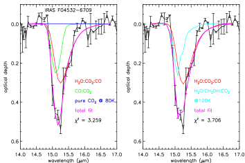
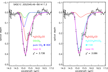
Figure 5: CO₂ profiles and best fits to the observed profiles (magenta), using a combination of either polar and apolar ices (left) or polar and annealed ices (right) — see text for explanation. The different components are color-coded as follows: water-rich (red), CO-rich (green), pure CO₂ (blue) and annealed (cyan). Reduced $\chi^{2}$ values are also given. Objects are plotted in order of decreasing total column density from top to bottom (Table 4).

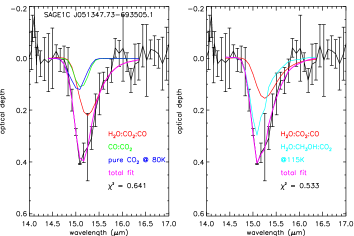
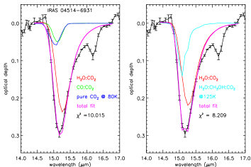
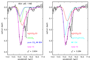
Figure 5: Continued.

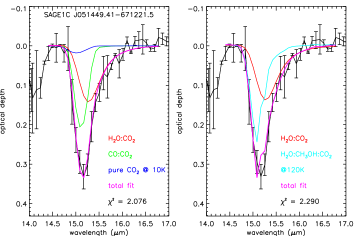
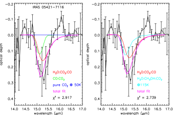
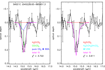
Figure 5: Continued.

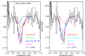
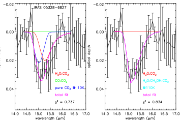
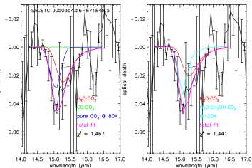
Figure 5: Continued.

Each observed CO₂ profile is modelled in two ways as described previously. Figure 5 shows the resulting fitted profiles. Table 4 lists relevant fitted parameters as well as the total CO₂ column density (see next section) and the percentages (in terms of column density) for each component. For three YSOs (MSX LMC 464, IRAS 05246-7137, and SAGE1C J054059.29$-$704402.6) the optical depth spectra were not deemed of good enough quality to fit meaningful models. Figure 6 shows their CO₂ profiles, and Table 4 lists the column densities.

The spectra of the remaining 12 YSOs in the sample are well fitted by the combinations of the lab profiles. Some objects exhibit features at $\sim$ 15.6 $\mu$m (e.g., SAGE1C J052546.49$-$661444.3 and MSX LMC 1786) and $\sim$ 16.2 $\mu$m (IRAS 04514$-$6931) that none of the model components can reproduce (Figure 4). There is a [Ne iii] emission line at 15.56 $\mu$m and a weak PAH feature at 15.9 $\mu$m. Therefore it is possible that these features are artifacts related to these two emission lines, either from the object itself or from its sky background.

The fitted profiles show that we are not able to distinguish between the different H₂O- and CO-rich mixtures used: similarly good fits are possible if the H₂O:CO₂ component is replaced by the H₂O:CO₂:CO mixture or the CO:CO₂ is replaced by CO:O₂:CO₂. There is also only a negligible difference in the fits when using the three available temperatures for pure-CO₂ ice. Accordingly, we make no such distinctions in Table 4, referring only to H₂O-rich (polar), CO-rich (“apolar1”) and pure-CO₂ (“apolar2”) components. When the polar + annealed combination is used, laboratory temperatures $\gtrsim$ 100 K are required, consistent with thermally processed mixtures in which CO₂ ice is segregated.

For seven YSOs the two strategies provide equally good results in terms of $\chi^{2}$ minimization. For two YSOs the polar + apolar modeling fits their spectra better while for three other objects the polar + annealed combination performs better. Gerakines et al. (1999) found that the combination of polar + annealed components fitted the data of their Galactic sample better, and suggested that this indicated that ice processing has occurred. We believe that for our data we cannot make this particular discrimination. The laboratory components are obviously very different, but the loss of spectral detail at the LL resolution and the combination of multiple components limits what we can discriminate.

In most cases, the two methods agree well on the amount of water-rich ice required. The majority of YSOs have a large fraction of CO₂ locked into H₂O-rich ice: for eight of the twelve fitted objects the polar component accounts for $\sim$ 45 $-$ 75% in column density. This is consistent with what is observed for Galactic YSOs (e.g., Pontoppidan et al., 2008; Gerakines et al., 1999). For the other four objects either no water-rich ice is required or the two strategies do not agree on how much is necessary. The polar component provides the dominant contribution to the red wing of the CO₂ profile (Figure 4). When contrast in this region is low (as is the case for SAGE1C 045228.65$-$685451.3, IRAS 05452$-$6924, and IRAS 05328$-$6827), it becomes more difficult to determine the contribution of the polar component. We test this effect by adding noise to one of our best profiles and re-fitting it: the profile looks narrower, and the amount of the polar CO₂ ice is not well constrained. The spectrum of SAGE1C J052546.49$-$661444.3 is of good quality, but it is also dominated by the feature at $\sim$ 15.52 $\mu$m.

If we consider the polar + apolar fits, a contribution from pure-CO₂ ice is present for all but two fitted YSOs; it typically accounts for 20 $-$ 50% of the total column density. Similarly, the CO-rich component is present in 10 profiles. Unlike Pontoppidan et al. (2008), we have difficulty in constraining the CO₂:CO concentration ratio for the CO-rich component in the profiles individually. However, there seems to be a tendency in the sample for high CO₂:CO ratios. If we consider the polar + annealed fits, a contribution from processed ices is needed in all cases.

4.3.3 CO₂ ice column density

Table 4 lists computed column densities adopting a band strength A = 1.1 $\times$ 10^-17 cm molecule^-1 (Gerakines et al., 1995); CO₂ column densities are in the range 0.45 $-$ 16 $\times$ 10¹⁷ cm^-2. Uncertainties listed in the table are statistical only. Different choices in defining the underlying continuum can change the measured column densities by $\sim$ 15%.

We can compare our new CO₂ column density measurements for IRAS 05240$-$6809, SAGE1C J052546.49$-$661411.3, and SAGE1C J051449.41$-$67221.5 with measurements performed with the low-resolution spectrograph ($R$ $\sim$ 20) on board AKARI for the 4.3-$\mu$m CO₂ stretching mode (Shimonishi et al., 2008). Their measurements suffered from very large uncertainties (at least 50%, see Table 4); both sets of measurements are consistent within the quoted uncertainties, however our measurements bring the estimated CO₂ column densities down considerably.

For those three objects, Shimonishi et al. (2008) also obtained water ice column densities — for IRAS 05240$-$6809 they do not tabulate a value for the column density, but we estimate it roughly from their Figure 1, $\sim$ 40 $\times$ 10¹⁷ cm^-2 with an assumed error of 25%. Van Loon et al. (2005b) measured the column density of water ice in IRAS 05328$-$6827; we re-estimate this column density using their spectrum and obtain 3.26 $\pm$ 0.27 $\times$ 10¹⁷ cm^-2. For these four YSOs (IRAS 05240$-$6809, SAGE1C J052546.49$-$661411.3, SAGE1C J051449.41$-$67221.5 and IRAS 05328$-$6827) we combine our CO₂ measurements with the H₂O measurements. Shimonishi et al. (2008) computed CO₂ and water column densities for a further three objects. Thus there are now seven YSOs in the LMC with column densities measured for both ice species. There is a strong positive correlation between the CO₂ and H₂O column densities for Galactic YSOs; in the next section we compare the measurements for YSOs in the LMC and the Galaxy.

4.4 The 5$-$7 $\mu$m ice band

The 6- and 6.8-$\mu$m ice bands dominate the 5$-$7 $\mu$m range in YSOs. Even though first identified by Puetter et al. (1979), their carriers are still not conclusively identified. The main contributor to the 6-$\mu$m component is the bending mode of water (e.g., Tielens et al., 2004). However, the column densities for the 3- and 6-$\mu$m water bands were found to be discrepant, with the 6-$\mu$m band often much too deep (e.g., Keane et al., 2001). Other ice species like formic acid (HCOOH), formaldehyde (CH₂O), and ammonia (NH₃) may contribute to the depth of the 6-$\mu$m feature (e.g., Knez et al., 2005; Boogert et al., 2008; Zasowski et al., 2009). Further, the 6-$\mu$m bending mode might be sensitive to the presence of both CO₂ and CO in the ice matrices (Öberg et al., 2007; Bouwman et al., 2007), which in some sources could account for some of the excess absorption at 6 $\mu$m (Knez et al., 2005). The ice component at 6.8 $\mu$m is now believed to be due mostly to ammonium (NH${}_{4}^{+}$), with a smaller contribution from methanol (CH₃OH) (Boogert et al., 2008).

In Section 4.1 we discussed how PAH and H₂ emission have also important spectral signatures in the 5 $-$7 $\mu$m spectral range, in particular the strong 6.3-$\mu$m PAH feature. Spoon et al. (2002) have shown that weak water ice features at 6 $\mu$m are effectively masked in the presence of a strong PAH emission spectrum (their Figure 1). As a large fraction of our sample shows significant PAH emission, this effect limits our ability to identify ice absorption in this spectral range. A quick inspection of the LMC sample of Seale et al. (2009) reveals that the majority of the objects that show CO₂ ice also show prominent PAH emission.

Boogert et al. (2008) and Zasowski et al. (2009) recently analyzed IRS high-resolution spectra of Galactic YSOs and found little or no sign of significant PAH emission. However these samples are mainly of low-luminosity objects. Thus PAH emission, if excited by the central object, would not dominate. In the higher-luminosity ISO sample discussed by Gibb et al. (2004) some objects show PAH emission, even though not as prominent as in our LMC sample.

In spite of the fact that there is a global dearth of PAH emission in metal-poor galaxies (Madden et al., 2006), we believe that the reason why PAH emission is so readily observed in YSOs in the LMC has to do with the issue of spatial resolution. As discussed in Section 2, observations YSOs in the LMC probe a larger region of the objects’ environment compared to Galactic sources. Extended PAH emission can then easily appear superimposed onto the spectra of icy mantles. A Galactic example of such “source confusion” in star forming environments is Mon R2: its ISO-SWS spectrum shows contributions from both an embedded YSO with ice and silicate absorption (Mon R2 IRS 1) and an ultracompact H ii region (Mon R2 IRS 2) (Spoon et al., 2004, their Fig 4). Such problem is also well documented in the analysis of the spectra of ultra-luminous infrared galaxies (e.g., Spoon et al., 2002, 2004).

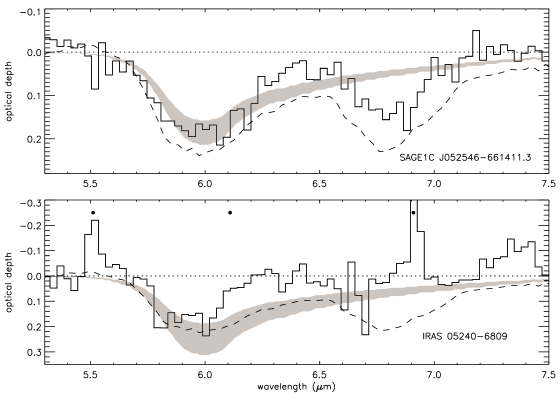
Figure 7: Optical depth in the 5 $-$ 7 $\mu$m region, respectively for SAGE1C J052546.49$-$661411.3 and IRAS 05240$-$6809. The filled circles indicate the position of unresolved H₂ lines, of which two are clearly present in the spectrum of IRAS 05240$-$6809. We also show typical laboratory ice models for pure water (Hudgins et al., 1993), scaled to match the water column densities measured using the 3-$\mu$m feature (Table 4), taking into account their error bars (shaded areas). The dashed line is an optical-depth spectrum for the Galactic YSO IRAS 04016+2610 from Zasowski et al. (2009) showing water ice and the additional ice feature at 6.8 $\mu$m (spectrum scaled by a factor 1.5). Both LMC objects clearly show the presence of water ice and SAGE1C J052546.49$-$661411.3 also shows the 6.8-$\mu$m feature (see text).

Figure 7 shows the spectra for the two objects in the sample for which we could identify the H₂O ice absorption band at 6 $\mu$m: IRAS 05240 $-$6809 and SAGE1C J052546.49$-$661411.3. None of these spectra show obvious PAH emission but IRAS 05240 $-$6809 shows unresolved H₂ emission. These YSOs show two of the largest CO₂ ice column densities ($\gtrsim$ 9 $\times$ 10¹⁷ cm^-2, Table 4), and thus should also have the largest water ice column densities (see next section). IRAS F04532$-$6709 shows similarly large CO₂ column density, but we cannot detect the 6-$\mu$m water ice feature which is probably hidden by PAH emission.

We also show in Figure 7 typical laboratory ice spectra ($T=40$ K, Hudgins et al., 1993) scaled to match published water column densities measured for the 3-$\mu$m feature (Table 4) and taking into account the measurement uncertainties (shaded areas in the figure). We have not made any allowance for the variable contribution of other ice species to the water ice band as described above. It is immediately obvious that, in particular between 6 and 6.5 $\mu$m, the observed features are not deep enough to match the published water column densities. This suggests a deficiency in our continuum determination in this region. The figure also shows an example of a Galactic YSO from Zasowski et al. (2009) for the complete 5 $-$ 7 $\mu$m range, highlighting the contribution of the 6.8-$\mu$m ice band. The spectrum of SAGE1C J052546.49$-$661411.3 does indeed show this feature, likely attributed to NH${}_{4}^{+}$ (Boogert et al., 2008).

5 Discussion

In this section we compare in more detail the properties of ices in the LMC YSOs to Galactic samples and interpret our results in terms of the star formation environment in the LMC.

5.1 Observed properties of the CO₂ ice profiles

As we have seen in Section 4.4, a large fraction of CO₂ ice is locked in a water-rich ice matrix, with a possible contribution from CO₂ ice in a CO-rich layer. Figure 8 compares the fraction of CO₂ ice in the water-rich component for the LMC sample and Galactic samples from the literature: high-luminosity YSOs and background sources(Gerakines et al., 1999; Whittet et al., 2009) and low-luminosity YSOs (Pontoppidan et al., 2008). The column densities for this component are derived using the polar + apolar modelling approach (Section 4.3.2) for all samples. In the Galaxy, luminous YSOs and background sources display a larger fraction of CO₂ ice in the water-rich component ($\sim$ 85%) when compared to low-luminosity sources ($\sim$ 70%). The typical fraction for the LMC objects is $\sim$ 60%. This suggests that, even though both in the LMC and in the Galaxy the water-rich component is the major contributor to CO₂ ice, its fraction might be smaller for the LMC sources. However, we note that the LMC sample is small, and systematic uncertainties could bring the samples into better agreement. Even though a similar profile decomposition was used to isolate the water-rich contribution, there are differences in the modelling approach (e.g., number and properties of the components considered).

A contribution from pure-CO₂ ice is also needed to fit the majority of the profiles. Whether this contribution arises from inclusions in annealed ices or a pure-CO₂ layer resulting from CO desorption is less obvious. If CO₂ forms in either water- and/or CO-rich ice mixtures as has been widely suggested, then the presence of pure CO₂ diagnoses thermal processing. Therefore, our analysis of the morphology (i.e. shape and composition) of the 15.2-$\mu$m CO₂ ice profiles of a sample of embedded YSOs in the LMC reveals only marginal differences when compared to Galactic YSOs. In the next section we discuss the concentration of CO₂ ice in relation to water ice.

5.2 CO₂ ice abundance in LMC

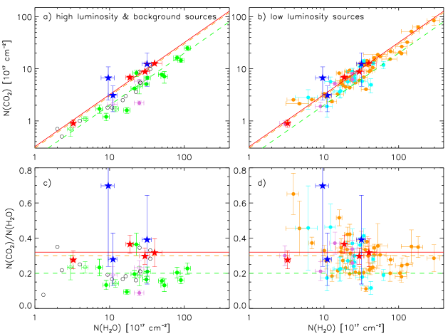
Figure 9: CO₂ ice versus H₂O ice column densities. We compiled measurements from the literature for Galactic sources (circles): Gerakines et al. (1999, green), Nummelin et al. (2001, pink), Zasowski et al. (2009, cyan), Pontoppidan et al. (2008, gold), and Whittet et al. (2007, 2009) and Knez et al. (2005) (black). Filled circles are YSOs while open circles are background sources (i.e. quiescent sightlines). Star symbols are the seven LMC measurements: from Shimonishi et al. (2008, blue stars) and our CO₂ ice measurements combined with literature H₂O ice measurements (red stars). The full lines are median ratios N(CO₂)/N(H₂O) for Galactic high-luminosity and background sources ($\sim$ 0.2, green), Galactic low-luminosity sources ($\sim$ 0.3, gold) and LMC sources ($\sim$ 0.32, red) — see text for full explanation.

Using compiled column-density measurements (Figure 9), we recompute the Galactic $N({\rm CO}_{2})/N({\rm H_{2}O})$ ratio. Filled and open circles are for Galactic YSOs and background sources, respectively. Measurements for LMC YSOs are shown as star symbols. The YSOs in the Gerakines et al. (1999) sample are luminous, while those in the Nummelin et al. (2001), Pontoppidan et al. (2008) and Zasowski et al. (2009) samples are low-luminosity objects. The Knez et al. (2005) and Whittet et al. (2007, 2009) samples are exclusively of background sources.

Measurements of the column density of CO₂ ice are for either the 15.2-$\mu$m bending mode (Gerakines et al., 1999; Knez et al., 2005; Pontoppidan et al., 2008; Zasowski et al., 2009; Whittet et al., 2009) or the 4.3-$\mu$m stretching mode (Nummelin et al., 2001; Shimonishi et al., 2008). Measurements of H₂O ice are for the 3-$\mu$m stretching mode, except for Zasowski et al. (2009), who used the 6-$\mu$m bending mode. They did not account for the contribution of other ice species to the 6-$\mu$m optical depth. Therefore, they have probably overestimated the column density of water ice. To compare them with the other samples, we need to scale them accordingly. Boogert et al. (2008) compared the column densities of water ice at 3 and 6 $\mu$m, and they found that the 6-$\mu$m value is on average higher than the 3-$\mu$m value by a factor of 1.74 (the median of 49 sources; the standard deviation is 0.62). The adjusted column densities of Zasowski et al. (2009) appear in Figure 9. We have also converted their column densities for CO₂ ice (computed using A = 1.5 $\times$ 10^-17 cm molecule^-1 ) to use the same band strength as the other measurements discussed here (A = 1.1 $\times$ 10^-17 cm molecule^-1).

Figure 9 shows the strong correlation between $N({\rm CO}_{2})$ and $N({\rm H_{2}O})$. The median value for the number density ratio is $N({\rm CO}_{2})/N({\rm H_{2}O})$ $\sim$ 0.2 for luminous Galactic YSOs and background sources (Gerakines et al., 1999; Whittet et al., 2007; Knez et al., 2005; Whittet et al., 2009). For low-luminosity Galactic YSOs, that ratio is $N({\rm CO}_{2})/N({\rm H_{2}O})$ $\sim$ 0.3 (Nummelin et al., 2001; Boogert et al., 2004; Pontoppidan et al., 2008) with a very large spread. Zasowski et al. (2009) reported a ratio of 0.16; however if the correction factor derived in the previous paragraph is applied to the measured water column densities then that ratio becomes 0.28, fully consistent with the previous value. In fact, the right-hand panels (b and d) in Figure 9 show that, with this correction, the low-luminosity measurements are essentially indistinguishable for the different samples. Note that there is a larger scatter for the measurements of low-luminosity objects when compared to the high-luminosity and background sample. Therefore, Figure 9 suggests a clear difference between the high-luminosity YSO and background samples, and the low-luminosity YSO samples (see also Pontoppidan et al., 2008).

Shimonishi et al. (2008) estimated a ratio $N({\rm CO}_{2})/N({\rm H_{2}O})$ $\sim$ 0.45 $\pm$ 0.17 for five LMC YSOs. As mentioned previously, we revised some of Shimonishi’s estimates downwards. For the seven LMC YSOs with both column-density measurements we estimate a median ratio $N({\rm CO}_{2})/N({\rm H_{2}O})$ = 0.32 $\pm$ 0.15 (1 $\sigma$). A single Shimonishi’s measurement drives this large spread, it would otherwise be $N({\rm CO}_{2})/N({\rm H_{2}O})$ = 0.32 $\pm$ 0.05 (1 $\sigma$). Estimated total luminosities in our sample are 5 $-$50 $\times$ 10³ L_⊙, comparable to the massive YSO sample in the Galaxy. Figure 9 (left panels) shows that if the high-luminosity Galactic and LMC samples are compared the $N({\rm CO}_{2})/N({\rm H_{2}O})$ ratio is higher in the LMC, by a factor 1.6. It is curious, however, that the ratio measured for the LMC objects is consistent with the low-luminosity Galactic sample. Note that column-density measurements do not depend on any modelling details but are prone to systematic uncertainties, namely in the continuum determination, that are generally difficult to quantify.

One should investigate the homogeneity of the samples discussed here. The LMC sample is restricted to very luminous YSOs, and it should, in terms of luminosity at least, be comparable to the sample of luminous Galactic YSOs observed with ISO. Spitzer studies of star formation concentrated on nearby star-forming regions, molecular clouds and isolated globules that form predominantly intermediate- and low-luminosity objects. These low-luminosity Galactic samples include a variety of evolutionary stages from more embedded YSOs to Herbig AeBe, T Tauri and zero-age main-sequence stars. The different timescales involved in the formation of objects with different luminosity may leave an imprint on the observed ice chemistry. Furthermore, YSOs in the LMC should in general appear more evolved due to the smaller dust column density in LMC objects when compared to Galactic objects.

Galactic and LMC measurements sample different spatial scales (Section 2), from a few parsecs in the LMC to milliparsecs in the Galaxy. If there is a gradient of ice abundances between the more immediate YSO cocoon and the wider molecular environment in which it is immersed (Pontoppidan, 2006), then the fact that ice properties are integrated over different spatial scales could affect global abundance ratios.

Such issues should be considered, since models of molecular clouds and their chemical evolution during the star formation process suggest that both temporal and radial variations of molecular concentrations are important (e.g., Lee et al., 2004; Rodgers & Charnley, 2003; Garrod et al., 2008; van Weeren et al., 2009; Hollenbach et al., 2009). Lee et al. (2004) singles out CO abundances (and the balance of its gas and solid phases) as particularly critical in determining the chemistry of star-forming cores. Even though they did not explicitly discuss CO₂ formation, the evolution of the two molecules is obviously closely linked. The balance of water in the gas phase and in ice form is also controlled by time- and space-dependent effects (Hollenbach et al., 2009).

5.3 The star formation environment in the LMC

The focus of this project is how the metal-poor star-formation environment in the LMC influences the chemistry of the envelopes that surround YSOs. Thus we now look at what is known about the environment in molecular clouds in the LMC.

The structure of Giant Molecular Clouds (GMCs) in metal-poor galaxies including the LMC is different from that in the Galaxy. Observations suggest that in metal-poor galaxies there are large reservoirs of H₂ that are not traced by CO (e.g., Israel, 1997). The magnitude of this H₂-to-CO excess was found to depend strongly on both metallicity and strength of the radiation field. This has been interpreted as the result of selective photodissociation of CO in the outer parts of metal-poor GMCs (e.g., Israel, 1997; Bolatto et al., 1999): H₂ readily self-shields while CO is shielded from the photodissociating radiation mostly by dust, which is less abundant at low metallicities. In this case, CO emission would trace only the inner parts of metal-poor GMCs. If CO cores are smaller in the LMC, due to the harsher UV radiation field (e.g., Welty et al., 2006) and lower dust abundance (e.g., Bernard et al., 2008) then we could naively expect CO₂ production to be reduced. A lower production rate of CO₂ could just result from the lower abundance of gas-phase CO observed in the LMC (e.g., Bel et al., 1986; Fukui et al., 2001; Pineda et al., 2009). It could also result from a smaller density of dust grains that act as seeds for the surface chemistry. Both effects would then tend to reduce the value of $N({\rm CO}_{2})/N({\rm H_{2}O})$. However as described above this is not what we observed in the LMC.

The formation of CO₂ ice in a wide variety of environments (e.g., both quiescent sightlines and low- and high-luminosity YSOs) argues against the need for enhanced radiative processing. Still, laboratory experiments do show that UV irradiation enhances CO₂ production (e.g., D’Hendecourt et al., 1986), and models of diffusive surface chemistry can produce high CO₂ densities at slightly elevated temperatures (e.g., Ruffle & Herbst, 2001). The LMC has a stronger ambient UV radiation field when compared to the Galaxy (by a factor of 1 $-$10, Bel et al., 1986; Welty et al., 2006). As a result of the stronger radiation field, the average ISM dust temperature is also generally higher in the LMC (12 $\lesssim$ $T_{\rm d}$ $\lesssim$ 35 K, Bernard et al., 2008) than in the Galaxy (19 $\lesssim$ $T_{\rm d}$ $\lesssim$ 25 K, Reach et al., 1996) — dust temperatures in cloud cores are lower than in the diffuse ISM. Both these effects could increase CO₂ production and increase $N({\rm CO}_{2})/N({\rm H_{2}O})$, consistent with what is observed.

We should also consider the possibility that the formation of water ice is somewhat inhibited in the LMC. The largest column density of water ice measured so far in the LMC is $\sim$ 5 $\times$ 10¹⁸ cm^-2 (Shimonishi et al., 2008). This is below the highest column densities measured towards Galactic YSOs, 10 $-$30 $\times$ 10¹⁸ cm^-2 (Gibb et al., 2004; Pontoppidan et al., 2008). Due to the small number of LMC objects investigated to date and possible selection effects this may not be a significant difference. Water ice seems to form rather easily in molecular clouds. However the A_V-threshold for water ice formation ($A_{\rm V}$ $\sim$ 3 mag for typical Galactic molecular clouds) is affected by the strength of the incident radiation field and dust temperature (Hollenbach et al., 2009). Still, it is difficult to see how water ice formation could be inhibited when CO₂ ice formation is not.

6 Summary and final remarks

We analyzed Spitzer-IRS spectra of a sample of embedded young stellar objects in the LMC, obtained as part of the SAGE-Spec Legacy program. We selected sources for this analysis based on the shape of their mid-IR continuum and the presence of the bending mode of CO₂ ice at 15.2 $\mu$m; a total of 15 sources were included, with three CO₂ ice detections considered marginal only ($<$ 3-$\sigma$). Based on modelling of the objects’ SEDs, we characterize the LMC YSOs as luminous and still in the early embedded stages of evolution.

A large fraction of the spectra of the LMC YSOs show prominent PAH emission. This does not necessarily mean that the sources are more evolved, ultracompact H ii regions. The Spitzer-IRS spatial resolution combined with the distance to the LMC implies that our spectra sample a relatively large fraction of the YSOs’ environment (a few square parsecs) when compared to Galactic YSOs, and thus PAH emission frequently appears superimposed onto the spectra of embedded YSOs. This makes the identification of the 5$-$7 $\mu$m ice band difficult. We detect water ice at 6 $\mu$m for two YSOs and the 6.8-$\mu$m feature (likely due to ammonium) in a single object.

It is usually believed that CO₂ forms on icy mantles, in water-dominated (polar) and/or CO-dominated (apolar) ice matrices. In Galactic YSOs, the water-rich component is the most abundant. These components exhibit a distinct morphology allowing a multi-component analysis of the observed profiles. The double-peaked structure found in the CO₂ ice profiles towards YSOs in the Galaxy is a signature of thermal processing, via which the CO₂ segregates from the other ice constituents. There are two types of modelling usually found in the literature: a dominant water-rich component is combined with either one or more apolar (CO- or CO₂-dominated) components, or with an annealed ice component (water, CO₂ and methanol in equal parts). Accordingly, we model the observed profiles of CO₂ ice towards LMC YSOs in these two ways, using databases of laboratory ice profiles available in the literature. We find that at the lower-resolution of the IRS LL mode, a considerable amount of detail is lost from the laboratory spectra. Thus our comparison of the two types of modelling is not conclusive.

We find that the CO₂ ice towards LMC YSOs is also dominated by the water-rich component, and they also require a contribution from pure CO₂ ice. Thus in terms of general morphology and composition the CO₂ ice towards LMC YSOs is similar to that observed towards Galactic YSOs. There are however two possible differences. First, there is a hint that the fraction of CO₂ ice locked into a water-rich matrix is smaller in the LMC. Furthermore, the column density ratio $N({\rm CO}_{2})/N({\rm H_{2}O})$, available for some of the targets, seems larger in the LMC.

One puzzling fact becomes noticeable when the available Galactic samples are separated into luminous and low-luminosity YSOs. The YSOs in our LMC sample are luminous and thus should in principle be compared to the Galactic high-luminosity sample. However, it is apparent from Figures 8 and 9 that the properties of the CO₂ profiles observed towards LMC YSOs more resemble those of low-luminosity Galactic YSOs rather than those of the high-luminosity Galactic YSOs, both in terms of water-rich fraction and concentration ratio. Admittedly the size of the LMC sample is small thus these results are tentative for now. We discuss how the temporal and spatial evolution of the physical conditions in molecular clouds can affect the observed properties of the different samples we compare.

We also discuss the implications of our results in terms of the star formation conditions in molecular clouds in the LMC. The ISM of the LMC has lower metallicity than the Galactic ISM ($Z_{\rm LMC}\sim 0.4$ Z_⊙). This affects the conditions in molecular clouds in the LMC in two parallel ways. On one hand there is less carbon and oxygen, and less dust. On the other hand, due to reduced shielding, the physical conditions in molecular clouds are harsher.

CO in the gas phase is less abundant, and the gas:dust ratio is larger by a factor 2 to 3 in the LMC than in the Galaxy. Observations also suggest that CO cores are smaller in the LMC, the result of selective photodissociation of CO in the outer parts of GMCs. If water ice abundance is unchanged, these effects would conspire to reduce the ratio of CO₂ ice to water ice in the LMC. This is clearly not what we observe. On the other hand, the twined facts that the UV radiation field is stronger and the average dust temperature is higher in the LMC could increase CO₂ production, which would be consistent with what we see in our sample.

Our results are tantalizing but not yet conclusive. We suggest that dust temperature could be responsible for observed differences between the LMC and the Galaxy. CO ice is more volatile than CO₂ and the CO profiles can be used as an indicator of thermal processing if different components correspond to environments of different volatility. The suggestion is that CO ice is more sensitive to the relatively small dust temperature differences mentioned previously. Furthermore, the possible increases in UV photolysis and thermal processing are related to metallicity. We have obtained Spitzer-IRS observations in the SMC and complementary ground-based data in both LMC and SMC, with the goal to incorporate CO ice profiles in our analysis, and to extend these studies to the even more metal-poor environment of the SMC.

Table 1: Sample of embedded LMC YSOs, with groundbased optical and near-IR photometry. $UBVI$ and $JHK$ fluxes are from the MCPS and IRSF catalogs, respectively (Zaritsky et al., 2004; Kato et al., 2007).

ID	RA	DEC	FU	FB	FV	FI	FJ	FH	FK
	(${}^{h\,\,m\,\,s}$)	(${}^{d\,\,m\,\,s}$)	($\mu$Jy)	($\mu$Jy)	($\mu$Jy)	($\mu$Jy)	(mJy)	(mJy)	(mJy)
IRAS 04514$-$6931	04:51:11.47	$-$69:26:46.9	58.6 $\pm$ 10.0	179.4 $\pm$ 18.7	324.4 $\pm$ 40.7	194.3 $\pm$ 19.5	0.168 $\pm$ 0.006	0.396 $\pm$ 0.018	0.730 $\pm$ 0.067
SSTISAGE1C J045228.65$-$685451.3	04:52:28.65	$-$68:54:51.3	5.0 $\pm$  1.8	26.4 $\pm$  2.4	61.5 $\pm$  4.6	111.1 $\pm$  7.7	0.068 $\pm$ 0.007	0.275 $\pm$ 0.020	0.748 $\pm$ 0.041
IRAS F04532$-$6709	04:53:11.03	$-$67:03:56.0	34.2 $\pm$  3.7	56.6 $\pm$  4.1	107.6 $\pm$ 22.1	$\cdots$	0.112 $\pm$ 0.009	0.190 $\pm$ 0.018	0.323 $\pm$ 0.027
SSTISAGE1C J050354.56$-$671848.5	05:03:54.56	$-$67:18:47.7	50.1 $\pm$ 10.1	55.9 $\pm$  7.9	53.7 $\pm$  4.5	61.0 $\pm$  5.2	0.475 $\pm$ 0.009	2.034 $\pm$ 0.019	6.658 $\pm$ 0.061
SSTISAGE1C J051347.73$-$693505.1	05:13:47.79	$-$69:35:05.1	$\cdots$	$\cdots$	$\cdots$	$\cdots$	$\cdots$	$\cdots$	0.389 $\pm$ 0.037
SSTISAGE1C J051449.41$-$671221.5	05:14:49.41	$-$67:12:21.5	5.7 $\pm$  2.5	14.0 $\pm$  1.5	19.7 $\pm$  4.7	73.8 $\pm$  4.0	0.224 $\pm$ 0.008	1.112 $\pm$ 0.021	4.811 $\pm$ 0.133
IRAS 05240$-$6809	05:23:51.14	$-$68:07:12.4	$\cdots$	68.2 $\pm$ 10.4	780.4 $\pm$ 108.5	$\cdots$	5.936 $\pm$ 0.711	6.021 $\pm$ 0.388	13.158 $\pm$ 0.727
IRAS 05246$-$7137	05:23:53.95	$-$71:34:44.0	$\cdots$	$\cdots$	$\cdots$	$\cdots$	0.055 $\pm$ 0.004	0.484 $\pm$ 0.018	3.966 $\pm$ 0.037
MSX LMC 464	05:24:13.30	$-$68:29:59.0	143.6 $\pm$ 12.0	192.8 $\pm$ 18.3	255.1 $\pm$ 23.7	$\cdots$	1.765 $\pm$ 0.032	6.909 $\pm$ 0.127	20.231 $\pm$ 0.373
SSTISAGE1C J052546.49$-$661411.3	05:25:46.52	$-$66:14:11.3	6.0 $\pm$  1.4	15.5 $\pm$  1.7	34.2 $\pm$  2.0	58.8 $\pm$  6.6	0.110 $\pm$ 0.007	0.462 $\pm$ 0.017	3.254 $\pm$ 0.060
IRAS 05328$-$6827	05:32:38.59	$-$68:25:22.2	$\cdots$	$\cdots$	$\cdots$	$\cdots$	0.191 $\pm$ 0.007	0.028 $\pm$ 0.418	9.111 $\pm$ 0.168
MSX LMC 1786	05:37:28.07	$-$69:08:48.0	$\cdots$	18.4 $\pm$  2.4	27.6 $\pm$  3.7	$\cdots$	0.254 $\pm$ 0.012	0.611 $\pm$ 0.034	1.180 $\pm$ 0.076
SSTISAGE1C J054059.29$-$704402.6	05:40:59.29	$-$70:44:02.6	$\cdots$	31.1 $\pm$  6.4	26.6 $\pm$  3.8	31.9 $\pm$  3.5	$\cdots$	0.289 $\pm$ 0.032	0.780 $\pm$ 0.044
IRAS 05421$-$7116	05:41:25.08	$-$71:15:32.7	50.5 $\pm$  4.8	120.8 $\pm$  5.5	57.4 $\pm$  7.8	$\cdots$	0.423 $\pm$ 0.026	0.690 $\pm$ 0.044	1.285 $\pm$ 0.058
IRAS 05452$-$6924	05:44:50.23	$-$69:23:04.7	12.9 $\pm$  2.5	23.5 $\pm$  1.5	35.0 $\pm$  2.3	78.5 $\pm$  4.2	0.181 $\pm$ 0.007	0.321 $\pm$ 0.012	0.671 $\pm$ 0.025

Table 2: Sample of embedded LMC YSOs, with Spitzer IRAC and MIPS photometry from the SAGE catalog (Meixner et al., 2006). The last column provides alternative identifications and known classifications from the literature.

ID	F${}_{3.6\,\mu{\mathrm{m}}}$	F${}_{4.5\,\mu{\mathrm{m}}}$	F${}_{5.8\,\mu{\mathrm{m}}}$	F${}_{8\,\mu{\mathrm{m}}}$	F${}_{24\,\mu{\mathrm{m}}}^{b}$		F${}_{70\,\mu{\mathrm{m}}}$	F${}_{160\,\mu{\mathrm{m}}}$	Comments
	(mJy)	(mJy)	(mJy)	(mJy)	(mJy)		(mJy)	(mJy)
IRAS 04514$-$6931	5.72 $\pm$ 0.494	18.90 $\pm$ 0.547	52.70 $\pm$ 1.529	96.0 $\pm$ 6.386	2538.0 $\pm$ 16.590	2538.0 $\pm$ 16.590	15820 $\pm$ 127.40	1257 $\pm$ 336.70	MSX LMC 1200
SSTISAGE1C J045228.65$-$685451.3	3.21 $\pm$ 0.173	6.05 $\pm$ 0.169	10.80 $\pm$ 0.288	23.0 $\pm$ 0.514	198.3 $\pm$  1.364	217.4 $\pm$  1.064	1435 $\pm$  24.24	2793 $\pm$  81.96	YSO (1)
IRAS F04532$-$6709	2.03 $\pm$ 0.350	4.00 $\pm$ 0.171	9.10 $\pm$ 0.381	16.9 $\pm$ 0.880	391.3 $\pm$  2.158	350.1 $\pm$  2.214	2454 $\pm$  29.70	3815 $\pm$ 110.10
SSTISAGE1C J050354.56$-$671848.9	24.50 $\pm$ 0.475	35.60 $\pm$ 0.514	45.40 $\pm$ 0.869	64.5 $\pm$ 1.579	180.6 $\pm$  4.059	307.2 $\pm$  2.703	7374 $\pm$  72.46	1091 $\pm$ 385.10	YSO (1)
SSTISAGE1C J051347.73$-$693505.1	$\cdots$	3.13 $\pm$ 0.158	8.25 $\pm$ 0.417	17.6 $\pm$ 0.830	372.5 $\pm$  1.899	276.4 $\pm$  2.949	$\cdots$	$\cdots$	YSO (1)
SSTISAGE1C J051449.41$-$671221.5	19.20 $\pm$ 0.586	34.30 $\pm$ 0.651	51.20 $\pm$ 0.939	71.3 $\pm$ 1.238	281.7 $\pm$  1.634	294.8 $\pm$  1.674	1243 $\pm$  19.92	$\cdots$	YSO (1), ST4 (2)
IRAS 05240$-$6809	22.50 $\pm$ 0.685	33.40 $\pm$ 0.529	42.20 $\pm$ 0.860	56.8 $\pm$ 0.797	1216.0 $\pm$  6.113	1270.0 $\pm$  7.630	3962 $\pm$  42.34	1384 $\pm$  91.71	YSO (1), ST7 (2)
IRAS 05246$-$7137	34.50 $\pm$ 0.694	62.50 $\pm$ 1.799	92.90 $\pm$ 1.672	119.0 $\pm$ 1.877	342.6 $\pm$  1.588	348.2 $\pm$  2.042	1490 $\pm$  19.09	$\cdots$	YSO (1), MIPS-SED (3)
MSX LMC 464	63.60 $\pm$ 1.890	89.50 $\pm$ 2.576	122.00 $\pm$ 2.684	175.0 $\pm$ 4.752	868.0 $\pm$  4.333	668.0 $\pm$  4.412	6741 $\pm$  58.81	1961 $\pm$ 421.60	H ii? (4)
SSTISAGE1C J052546.49$-$661411.3	30.00 $\pm$ 0.668	56.60 $\pm$ 1.554	79.80 $\pm$ 1.430	115.0 $\pm$ 1.958	504.7 $\pm$  3.381	498.4 $\pm$  3.021	1417 $\pm$  34.56	17510 $\pm$ 363.90	YSO (1), ST3 (2)
IRAS 05328$-$6827	77.24 $\pm$ 3.294	148.20 $\pm$ 3.771	212.90 $\pm$ 3.233	261.7 $\pm$ 7.766	1070.0 $\pm$  5.392	919.3 $\pm$  5.637	3052 $\pm$  63.57	1113 $\pm$ 230.80	YSO (5), MIPS-SED (3)
MSX LMC 1786	11.20 $\pm$ 0.500	34.20 $\pm$ 0.784	88.10 $\pm$ 1.782	142.0 $\pm$ 2.200	1444.0 $\pm$  9.927	906.0 $\pm$ 11.460	4139 $\pm$ 231.90	2002 $\pm$ 636.10	30 Dor$-$17, MIPS-SED (3)
SSTISAGE1C J054059.29$-$704402.6	4.51 $\pm$ 0.202	10.30 $\pm$ 0.297	17.20 $\pm$ 0.480	29.5 $\pm$ 0.581	209.7 $\pm$  1.055	216.0 $\pm$  1.394	945 $\pm$  12.78	$\cdots$	YSO (1)
IRAS 05421$-$7116	3.70 $\pm$ 0.272	4.02 $\pm$ 0.120	7.55 $\pm$ 0.311	13.3 $\pm$ 0.949	331.4 $\pm$  1.770	329.0 $\pm$  2.454	2040 $\pm$  22.66	$\cdots$	YSO (1)
IRAS 05452$-$6924	2.36 $\pm$ 0.081	3.62 $\pm$ 0.114	8.58 $\pm$ 0.176	19.4 $\pm$ 0.406	674.9 $\pm$  3.158	659.3 $\pm$  3.609	2967 $\pm$  47.63	$\cdots$	YSO (1)

References. — (1) Whitney et al. (2008); (2) Shimonishi et al. (2008); (3) van Loon et al. (2009); (4) Kastner et al. (2008); (5) van Loon et al. (2005a).

Figure 1: Spitzer-IRS spectra of the 15 sources discussed in this work. From left to right and top to bottom, sources are shown in decreasing order of their measured IRAC flux at 5.8 $\mu$m. The insets in each graph show the spectral regions where ice bands can be found, namely the CO₂ ice feature at 15.2 $\mu$m (lower right corner) and the 5 $-$ 7 $\mu$m complex that includes the water ice O$-$H bending mode at 6 $\mu$m (upper left corner).

Figure 1: Continued.

Figure 1: Continued.

Table 3: Laboratory spectra used in the CO₂ ice fits from Ehrenfreund et al. (1997, E97) and White et al. (2009, W09).

mixture	temperature	reference
	(K)
H2O-rich polar ices
H2O:CO2 = 100:14	10	E97
H2O:CO2:CO = 100:20:3	20	E97
CO- or CO2-rich apolar ices
CO:CO2 = 100:4	10	E97
CO:CO2 = 100:8	10	E97
CO:CO2 = 100:16	10	E97
CO:CO2 = 100:21	10	E97
CO:CO2 = 100:23	10	E97
CO:CO2 = 100:26	10	E97
CO:CO2 = 100:70	10	E97
H2O:CO:CO2 = 1:50:56a	10	E97
CO:O2:CO2 = 100:50:4	10	E97
CO:O2:CO2 = 100:50:8	10	E97
CO:O2:CO2 = 100:50:16	10	E97
CO:O2:CO2 = 100:50:21	10	E97
CO:O2:CO2 = 100:50:32	10	E97
pure CO2	10	E97
pure CO2	50	E97
pure CO2	80	E97
annealed ices
H2O:CH3OH:CO2	5, 10,…, 135b	W09

Figure 6: CO₂ features for the three YSOs for which no fits with laboratory spectra were performed.

Table 4: Column densities and model fit information for the observed 15.2-$\mu$m CO₂ features. Uncertainties are statistical and do not include those associated with the continuum determination. Fit components are water-rich (polar), CO-rich (apolar1), pure-CO₂ (apolar2) and annealed ices. For each component percentages (in terms of column density) are given. For the polar + apolar ice fits the best-fit CO₂:CO ratio is provided; for the polar + annealed fits the best-fit annealed temperature is given. $\chi^{2}$ values for the fits are listed. Additional ice column densities are provided in the last column for the 4.3-$\mu$m feature of CO₂ and 3-$\mu$m feature of water ice, either from the literature (Shimonishi et al., 2008) or recomputed using published spectra (Shimonishi et al., 2008; van Loon et al., 2005a) — see text and table notes.

			polar + apolar fit					polar + annealed fit
ID	N(CO2)${}^{a}_{15\mu m}$		polar	apolar1	apolar2	CO2:CO	$\chi^{2}$	polar	annealed	T	T range	$\chi^{2}$	best fit	N(CO2)4.3μm	N(H2O)3μm
	1017 cm-2	$\sigma$	%	%	%			%	%	K	K			1017 cm-2
IRAS 05240$-$6809	12.69 $\pm$ 0.28	44.8	60 $\pm$  2	20 $\pm$  2	19 $\pm$  2	$\gtrsim$ 1.12	1.18	54 $\pm$  1	46 $\pm$  1	115	110 $-$ 120	3.35	apolar	55.3${}^{+40}_{-30}$	$\sim$ 40b
IRAS F04532$-$6709	9.91 $\pm$ 0.46	21.4	66 $\pm$  2	34 $\pm$  2	$\cdots$	$\gtrsim$ 1.12	3.26	66 $\pm$  3	34 $\pm$  3	120	115 $-$ 130	3.71	apolar
SAGE1C J052546.49$-$661411.3	8.83 $\pm$ 0.18	49.9	68 $\pm$  4	8 $\pm$  4	24 $\pm$  3	$\gtrsim$ 1.12	3.74	12 $\pm$  4	88 $\pm$  4	110	110 $-$ 115	3.09	annealed	15.5${}^{+13.8}_{-9.4}$	29.7${}^{+4.5}_{-4.6}$
SAGE1C J051347.73$-$693505.1	8.37 $\pm$ 0.93	9.0	59 $\pm$ 14	18 $\pm$ 14	23 $\pm$ 13	$\gtrsim$ 1.12	0.64	42 $\pm$  7	58 $\pm$  7	115	100 $-$ 130	0.53	$\cdots$
IRAS 04514$-$6931	7.99 $\pm$ 0.08	98.3	78 $\pm$  3	9 $\pm$  3	13 $\pm$  2	0.70 $\pm$ 0.47	10.01	73 $\pm$  1	27 $\pm$  1	125	110 $-$ 130	8.21	annealed
MSX LMC 1786	7.82 $\pm$ 0.47	16.6	54 $\pm$  3	27 $\pm$  4	19 $\pm$  3	$\gtrsim$ 1.12	3.90	40 $\pm$  2	60 $\pm$  2	115	110 $-$ 125	3.28	annealed
SAGE1C J051449.41$-$671221.5	6.84 $\pm$ 0.47	14.7	51 $\pm$  6	44 $\pm$  6	5 $\pm$  8	$\gtrsim$ 1.12	2.08	49 $\pm$  3	51 $\pm$  3	120	110 $-$ 130	2.29	$\cdots$	8.2${}^{+4.3}_{-3.7}$	18.7${}^{+2.3}_{-2.3}$
IRAS 05421$-$7116	4.95 $\pm$ 0.86	5.8	69 $\pm$  6	31 $\pm$  6	$\cdots$	$\gtrsim$ 1.12	2.92	60 $\pm$  8	40 $\pm$  8	115	110 $-$ 130	2.74	$\cdots$
SAGE1C J045228.65$-$685151.3	2.65 $\pm$ 0.44	6.0	$\cdots$	73 $\pm$ 22	27 $\pm$ 22	0.70 $\pm$ 0.57	3.72	$\cdots$	100	125	115 $-$ 130	3.61	$\cdots$
IRAS 05452$-$6924	2.36 $\pm$ 0.42	5.7	55 $\pm$ 14	20 $\pm$ 20	25 $\pm$ 10	0.10 $\pm$ 0.29	0.62	29 $\pm$  9	71 $\pm$  9	135	135 $-$ 135	0.58	$\cdots$
IRAS 05328$-$6827	0.90 $\pm$ 0.15	5.9	55 $\pm$  8	$\cdots$	45 $\pm$  8	$\cdots$	0.74	$\cdots$	100	110	110 $-$ 110	0.83	$\cdots$		3.26${}^{+0.27}_{-0.27}$c
SAGE1C J050354.56$-$671848.5	0.87 $\pm$ 0.22	4.0	50 $\pm$  8	$\cdots$	50 $\pm$  8	$\cdots$	1.47	46 $\pm$ 10	54 $\pm$ 10	120	110 $-$ 130	1.44	$\cdots$
SAGE1C J054059.29$-$704402.6	0.63 $\pm$ 0.77	0.8	$\cdots$					$\cdots$					$\cdots$
IRAS 05246$-$7137	0.46 $\pm$ 0.18	2.5	$\cdots$					$\cdots$					$\cdots$
MSX LMC 464	0.45 $\pm$ 0.17	2.7	$\cdots$					$\cdots$					$\cdots$

Figure 8: Fraction of CO₂ locked in the water-rich (polar) component, for the LMC sample (top) and Galactic YSOs and background sources (bottom). Galactic data come from Gerakines et al. (1999), Pontoppidan et al. (2008), and Whittet et al. (2009).

References

- Aguirre et al. (2003) Aguirre, J. E., et al., 2003, ApJ, 596, 273
- Banerji et al. (2009) Banerji, M., Viti, S., Williams, D. A., & Rawlings, J. M. C., 2009, ApJ, 692, 283
- Bel et al. (1986) Bel, N., Viala, Y. P., & Guidi, I., 1986, A&A, 160, 301
- Bergin & Tafalla (2007) Bergin, E. A., & Tafalla, M., 2007, ARA&A, 45, 339
- Bernard et al. (2008) Bernard, J.-P., et al., 2008, AJ, 136, 919
- Bolatto et al. (1999) Bolatto, A. D., Jackson, J.M., & Ingalls, J. G., 1999, ApJ, 513, 275
- Boogert et al. (2000) Boogert A. C. A., et al., 2000, A&A, 353, 349
- Boogert & Ehrenfreund (2004) Boogert A. C. A., & Ehrenfreund, P., 2004, in ASP Conference Series, Vol. 309, “Astrophysics of Dust”, A. N. Witt, G. C. Clayton & B. T. Draine. (eds.), p. 547
- Boogert et al. (2004) Boogert, A. C. A., et al., 2004, ApJS, 154, 359
- Boogert et al. (2008) Boogert A. C. A., et al., 2008, ApJ, 678, 985
- Bouwman et al. (2007) Bouwman, J., Ludwig, W., Awad, Z., Öberg, K. I., Fuchs, G. W., van Dishoeck, E. F., & Linnartz, H., 2007, A&A, 476, 995
- Buchanan et al. (2006) Buchanan, C. L., Kastner, J. H., Forrest, W. J., Hrivnak, B. J., Sahai, R., Egan, M., Frank, A., & Barnbaum, C., 2006, AJ, 132, 1890
- Chen et al. (2009) Chen, C.-H. R., Chu, Y.-H., Gruendl, R. A., Gordon, K. D., & Heitsch, F., 2009, ApJ, 695, 511
- Cutri et al. (2003) Cutri, R. M., et al., 2003, “The IRSA 2MASS All-Sky Point Source Catalog”, NASA/IPAC Infrared Science Archive
- D’Hendecourt et al. (1986) D’Hendecourt, L. B., Allamandola, L. J., Grim, R. J. A., & Greenberg, J. M., 1986, A&A, 158, 119
- Dijkstra et al. (2003) Dijkstra, C., Dominik, C., Hoogzaad, S. N., de Koter, A., & Min, M., 2003, A&A, 401, 599
- Ehrenfreund et al. (1997) Ehrenfreund, P., Boogert, A. C. A., Gerakines, P. A., Tielens, A. G. G. M., & van Dishoeck, E. F., 1997, A&A, 328, 649
- Ehrenfreund et al. (1998) Ehrenfreund, P., Dartois, E., Demyk, K., & D’Hendecourt, L., 1998, A&A, 339, 17
- Ehrenfreund et al. (1999) Ehrenfreund, P., et al., 1999, A&A, 350, 240
- Ehrenfreund & Fraser (2003) Ehrenfreund, P., & Fraser, H., 2003, in “Solid state astrochemistry” V. Pirronello, J. Krełowski & G. Manicó (eds.), NATO Science Series II: Mathematics, Physics and Chemistry, Dordrecht: Kluwer Academic Publishers, Vol. 120, p. 317
- Fraser et al. (2001) Fraser, H. J., Collings M. P., McCoustra M. R. S., & Williams D. A., 2001, MNRAS, 327, 1165
- Fukui et al. (2001) Fukui, Y., et al., 2001, PASJ, 51, 745
- Garrod et al. (2008) Garrod, R. T., Weaver. S. L. W., & Herbst, E., 2008, ApJ, 682, 283
- Gerakines et al. (1995) Gerakines P. A., Schutte, W. A., Greenberg, J. M., & van Dischoek, E. F., 1995, A&A, 296, 810
- Gerakines et al. (1999) Gerakines, P. A., et al., 1999, ApJ, 522, 357
- Gibb et al. (2004) Gibb, E. L. et al., 2004, ApJS, 151, 35
- Goldsmith & Langer (1978) Goldsmith, P. F., & Langer, W. D., 1978, ApJ, 222, 881
- Herbst & Leung (1986) Herbst, E., & Leung, C. M., 1986, MNRAS, 222, 689
- Hollenbach et al. (2009) Hollenbach, D., Kaufman, M. J., Bergin, E. A. & Melnick, G. J., 2009, ApJ, 690, 1497
- Hudgins et al. (1993) Hudgins, D. M., Sandford, S. A., Allamandola, L. J., & Tielens, A. G. G. M., 1993, ApJS, 86, 713
- Houck et al. (2004) Houck, J. R., et al., 2004, ApJS, 154, 18
- Ioppolo et al. (2008) Ioppolo, S., Cuppen, H. M., Romanzin, C., van Dischoeck, E. F., & Linnartz, H. , 2008, ApJ, 686, 1474
- Israel (1997) Israel, F. P., 1997, A&A, 328, 471
- Justtanont et al. (1998) Justtanont, K., Feuchtgruber, H., de Jong, T., Cami, J., Waters, L. B. F. M., Yamamura, I., & Onaka, T., 1998, A&A, 330, 17
- Kastner et al. (2008) Kastner, J. H., Thorndike, S. L., Romanczyk, P. A., Buchanan, C. L., Hrivnak, B. J., Sahai, R., & Egan, M., 2008, AJ, 136, 1221
- Kato et al. (2007) Kato, D., et al., 2007, PASJ, 59, 3
- Keane et al. (2001) Keane, J. V., Tielens, A. G. G. M., Boogert, A. C. A., Schutte, W. A., & Whittet, D. C. B., 2001, A&A, 376, 254
- Kemper et al. (2009) Kemper, F., et al., 2009, AJ, submitted
- Knez et al. (2005) Knez, C., et al., 2005, ApJ, 635, 145
- Lada (1987) Lada, C. J., 1987, in IAU Symp. 115, “Star Forming Regions”, M. Peimbert & J. Jugaku (eds), Dordrecht: Reidel
- Lee et al. (2004) Lee, J.-E., Bergin, E. A., & Evans, N. J. II, 2004, ApJ, 617, 360
- Madden et al. (2006) Madden, S. C., Galliano, F., Jones, A. P., Sauvage, M., 2006, A&A, 446, 877
- Markwardt (2009) Markwardt, C. B., 2009, “Non-Linear Least Squares Fitting in IDL with MPFIT”, in proc. Astronomical Data Analysis Software and Systems XVIII, ASP Conference Series, D. Bohlender, P. Dowler & D. Durand (eds.) (Astronomical Society of the Pacific: San Francisco), in press, arXiv:0902.2850v1
- Meixner et al. (2006) Meixner, M., et al., 2006, AJ, 132, 2268
- Moré (1977) Moré, J., 1977, “The Levenberg-Marquardt Algorithm: Implementation and Theory” in Numerical Analysis, vol. 630, ed. G. A. Watson (Springer-Verlag: Berlin), p. 105
- Murakami et al. (2007) Murakami, H., et al., 2207, PASP, 59, 369
- Nummelin et al. (2001) Nummelin, A., Whittet, D. C. B., & Gibb, E. L., ApJ, 558, 185
- Öberg et al. (2007) Öberg, K. I., Fraser, H. J., Boogert, A. C. A., Bisschop, S. E., Fuchs, G. W., van Dishoeck, E. F., Linnartz, H., 2007, A&A, 462, 1187
- Oliveira et al. (2006) Oliveira, J. M., van Loon, J. Th., Stanimirović, S., & Zijlstra, A. A., 2006, MNRAS, 372, 1509
- Oliveira (2009) Oliveira, J. M., 2009, in “The Magellanic System: Stars, , and Galaxies”, Proceedings of the International Astronomical Union, IAU Symposium, Volume 256, J. Th. van Loon & J. M. Oliveira (eds.), Cambridge University Press, p. 191
- Peeters et al. (2004) Peeters, E., Mattioda, A. L., Hudgins, D. M., & Allamandola, L. J., 2004, ApJ, 617, 65
- Pineda et al. (2009) Pineda, J. L., Ott, J., Klein, U., Wong, T., Muller, E., & Hughes, A., 2009, A&A, in press, arXiv0907.5186
- Pontoppidan (2006) Pontoppidan, K. M., 2006, A&A, 453, 47
- Pontoppidan et al. (2008) Pontoppidan, K. M., et al., 2008, ApJ, 678, 1005
- Puetter et al. (1979) Puetter, R. C., Russell, R. W., Willner, S. P., & Soifer, B. T., 1979, ApJ, 228, 118
- Reach et al. (1996) Reach, W. T., et al., 1996, A&A, 315, 381
- Rieke et al. (2004) Rieke, G. H., et al., 2004, ApJS, 154, 25
- Robitaille et al. (2006) Robitaille, T. P., Whitney, B. A., Indebetouw, R., Wood, K., Denzmore, P., 2006, ApJS, 167, 256
- Robitaille et al. (2007) Robitaille, T. P., Whitney, B. A., Indebetouw, R., & Wood, K., 2006, ApJS, 169, 328
- Rodgers & Charnley (2003) Rodgers, S. D., & Charnley, S. B., 2003, ApJ, 585, 355
- Ruffle & Herbst (2001) Ruffle, D. P., & Herbst, E., 2001, MNRAS, 324, 1054
- Seale et al. (2009) Seale, J. P., Looney, L. W., Chu, Y.-H., Gruendl, R. A., Brandl, B., Chen, C.-H. R., Brandner, W., & Blake, G. A., 2009, ApJ, 699, 150
- Shimonishi et al. (2008) Shimonishi, T., Onaka, T., Kato, D., Sakon, I., Ita, Y., Kawamura, A., & Kaneda, H., 2008, ApJ, 686, 99
- Smith et al. (2007) Smith, J. D. T., et al., 2007, ApJ, 656, 770
- Spoon et al. (2002) Spoon, H. W. W., Keane, J. V., Tielens, A. G. G. M., Lutz, D., Moorwood, A. F. M., & Laurent, O., 2002, A&A, 385, 1022
- Spoon et al. (2004) Spoon, H. W. W., Moorwood, A. F. M., Lutz, D., Tielens, A. G. G. M., Siebenmorgen, R., & Keane, J. V., 2004, A&A, 141, 873
- Tielens et al. (2004) Tielens, A. G. G. M., Allamandola, L. J., Bregman, J., Goebel, J., Witteborn, F. C., & D’Hendecourt, L. B., 1984, ApJ, 287, 697
- Tielens et al. (1991) Tielens, A. G. G. M., Tokunaga, A. T., Geballe, T. R., & Baas, F., 1991, ApJ, 381, 181
- Tielens (2008) Tielens, A. G. G. M., 2008, ARA&A, 46, 289
- van Broekhuizen et al. (2006) Van Broekhuizen, F. A., Groot, I. M. N., Fraser, H. J., van Dishoeck, E. F., & Schlemmer, S., 2006, A&A, 451, 723
- van Dishoeck (2004) van Dishoeck, E., 2004, ARA&A, 42, 119
- Van Kerckhoven et al. (2000) Van Kerckhoven, C., et al., 2000, A&A, 357, 1013
- van Loon et al. (2005a) van Loon, J. Th., et al., 2005a, MNRAS, 364, 71
- van Loon et al. (2005b) van Loon, J. Th., Marshall, J. R., & Zijlstra A. A., 2005b, A&A, 442, 597
- van Loon et al. (2008) van Loon, J. Th., Cohen, M., Oliveira, J. M., Matsuura, M., McDonald, I., Sloan G.C., Wood, P. R., & Zijlstra, A. A., 2008, A&A, 487, 1055
- van Loon et al. (2009) van Loon, J. Th. et al., 2009, AJ, submitted
- van Weeren et al. (2009) van Weeren, R. J., Brinch, C., & Hogerheide, M. R., 2009, A&A, 497, 773
- Welty et al. (2006) Welty, D. E., Federman, S. R., Gredel, R., Thorburn, J. A., & Lambert, D.L., 2006, ApJS, 165, 138
- Werner et al. (2004) Werner, M. W., et al., 2004, ApJS, 154, 1
- White et al. (2009) White, D. W., Gerakines, P. A., Cook, A. M., & Whittet, D. C. B., 2009, ApJS, 180, 182
- Whitney et al. (2008) Whitney, B. A., et al., 2008, AJ, 136, 18
- Whittet et al. (2007) Whittet, D. C. B., Shenoy, S. S., Bergin, E. A., Chiar, J. E., Gerakines, P. A., Gibb, E. L., Melnick, G. J., & Neufeld, D. A., 2007, ApJ, 655, 332
- Whittet et al. (2009) Whittet, D. C. B., Cook, A. M., Chiar, J. E., Pendleton, Y. J., Shenoy, S. S., & Gerakines, P. A., 2009, ApJ, 695, 94
- Williams (2003) Williams, D. A., 2003, in “Solid state astrochemistry”, V. Pirronello, J. Krełowski, & G. Manicó (eds.), NATO Science Series II: Mathematics, Physics, and Chemistry, Dordrecht: Kluwer Academic Publishers, Vol. 120, p. 1
- Zaritsky et al. (2004) Zaritsky, D., Harris, J., Thompson, I. B., & Grebel, E, K., 2004, AJ, 128, 1606
- Zasowski et al. (2009) Zasowski, G., Kemper, F., Watson, D. M., Furlan, E., Bohac, C. J., Hull, C., & Green, J. D., 2009, ApJ, 694, 459