Drag coefficient of a liquid domain in a two-dimensional membrane

Abstract

Using a hydrodynamic theory that incorporates a momentum decay mechanism, we calculate the drag coefficient of a circular liquid domain of finite viscosity moving in a two-dimensional membrane. We derive an analytical expression for the drag coefficient which covers the whole range of domain sizes. Several limiting expressions are discussed. The obtained drag coefficient decreases as the domain viscosity becomes smaller with respect to the outer membrane viscosity. This is because the flow induced in the domain acts to transport the fluid in the surrounding matrix more efficiently.

1 Introduction

Membrane components such as lipids and proteins are subject to Brownian motion, and the resulting diffusive process is an important mechanism for the transport of these materials. Consequently, it is generally believed that many biochemical functions in membranes are diffusion controlled processes. Up to now, the studies of diffusion in biomembranes have mainly concentrated either on protein molecules peters-82 ; lippincott-01 ; vrljic-02 ; reitz-01 ; gambin-06 or, more recently, on lipid domains sometimes called as “lipid rafts” klingler-93 ; oradd-05 ; cicuta-07 ; yanagisawa-07 ; sakuma-09 . Lipid domains appear due to a lateral phase separation between a liquid-ordered phase and a liquid-disordered phase veatch-05 , and have attracted much attention in relation to biological functionalities simons-97 .

In the theoretical studies, a protein molecule is assumed to be a rigid disk moving in a two-dimensional (2D) thin fluid sheet under low Reynolds number conditions. Saffman and Delbrück (SD) investigated this problem by considering a membrane that is sandwiched in between a three-dimensional (3D) fluid medium saffman-75 ; saffman-76 . They showed that the drag coefficient has only a weak logarithmic dependence on the disk radius in the small size limit. The SD model was further analyzed by Hughes et al. for the whole range of protein sizes, and they also obtained the asymptotic expression in the large size limit hughes-81 . The SD model was extended by Levine et al. for a viscoelastic film within an infinite viscous liquid, taking into account both in-plane and out-of-plane dynamics levine-02 ; levine-04 ; levine-04b .

On the other hand, Evans and Sackmann looked at a slightly different situation evans-88 , i.e., the diffusion of a protein molecule moving in a supported membrane (instead of a free membrane). The presence of the solid substrate is taken into account through a friction term in the Stokes equation. The equivalent hydrodynamic model was independently proposed by Izuyama who suggested that the momentum decay mechanism should generally exist for membranes surrounded by water izuyama-88 . Since a hydrodynamic equation with a momentum decay term was originally proposed by Brinkman for flow in porous media brinkman-47 , we call these approaches as the 2D Brinkman-type model. One of the advantages of the Brinkman model is that the drag coefficient can be analytically obtained over the whole range of disk sizes. In the small size limit, the SD model and the Brinkman model give the same logarithmic dependence. In biological systems, the Brinkman model can be more relevant because the cell membranes are strongly anchored to the underlying cytoskeleton, or are tightly adhered to other cells alberts .

Most of the previous work has concentrated on the problem of protein diffusion in a membrane for which the assumption of a rigid disk is reasonable. Liquid lipid domains, on the other hand, cannot be considered as rigid objects. A proper description should take into account the fluid nature and finite viscosity of the diffusing domain. It should be also noted that the viscosity of the lipid domain is different from that of the matrix oradd-05 . In this paper, we derive the drag coefficient of a circular liquid domain by taking into account its finite viscosity using the 2D Brinkman-type hydrodynamic equation. We show that the drag coefficient decreases as the domain viscosity becomes smaller. An analogous problem for a spherical drop of fluid was solved by Rybczyński and Hadamard about 100 years ago rybczynski-11 ; hadamard-11 . Some authors considered the hydrodynamics of Langmuir monolayer domains at the air/water interface by taking into account the fluid nature of the domain stone-95 ; lubensky-96 ; alexander-06 . In these works, however, the domain and the matrix viscosities are assumed to be the same, and the drag coefficient was not obtained dekoker . Although the rotational diffusion coefficient was also calculated for a rigid disk saffman-75 ; saffman-76 ; hughes-81 ; evans-88 , such a motion is irrelevant for a fluid domain which has an internal flow.

In the next section, we begin with a description of the 2D Brinkman model. In sect. 3, the solutions for the inside domain are connected to those for the outer membrane matrix through the appropriate boundary conditions. Then the drag coefficient is calculated for the entire region of the domain sizes. We also obtain several limiting expressions; some of which coincide with the previous results. Several discussions are provided in sect. 4.

2 Hydrodynamic model with momentum decay

The usual method of obtaining the diffusion coefficient $D$ from the drag coefficient $\zeta$ is to use the Einstein relation

$$D=\frac{k_{\rm B}T}{\zeta},$$ (1)

where $k_{\rm B}$ is the Boltzmann constant and $T$ the temperature. However, for a pure 2D system in the low Reynolds number regime, a linear relation between the velocity and drag force cannot be obtained landaulifshitz-flumech . This fact is due to the inability to simultaneously satisfy the boundary conditions both at the disk (cylinder) surface and at infinity within the Stokes approximation lamb-75 . Such a problem is known as the Stokes paradox which essentially originates from the constraint of momentum conservation in a pure 2D fluid.

Although a lipid bilayer membrane can be treated as a 2D viscous fluid, it is not an isolated system because the membrane is surrounded by a 3D fluid. Due to the coupling between the 2D membrane and the 3D fluid, the momentum within the membrane can leak away to the outer fluid. Such an effect can be taken into account through a momentum decay term in the equation of motion. This also enables the 3D fluid to be discarded and we can work in a pure 2D system. A hydrodynamic equation which is consistent with the total momentum decay is

$$\rho\left[\frac{\partial\mathbf{v}}{\partial t}+(\mathbf{v}\cdot\nabla)\mathbf{v}\right]=\eta\nabla^{2}\mathbf{v}-\nabla p-\lambda\mathbf{v}.$$ (2)

In the above, $\mathbf{v}$ and $p$ are the 2D velocity and pressure, respectively, while $\rho$ is the 2D membrane density, $\eta$ the membrane 2D viscosity, and $\lambda$ the momentum decay parameter. Notice that the usually reported membrane 3D viscosity is given by $\eta/h$, where $h$ is the membrane thickness. A more detailed derivation of eq. (2) in terms of the total momentum decay is given in seki-93 . Since 3D version of eq. (2) was originally used by Brinkman for flows in porous media brinkman-47 , we call it as 2D Brinkman equation. But it should be kept in mind that there is no real connection between porous media and membranes except from the momentum decay mechanism. For a typical flow in a membrane, we can adopt the Stokes approximation to eq. (2). Then we have

$$\eta\nabla^{2}\mathbf{v}-\nabla p-\lambda\mathbf{v}=0.$$ (3)

On the other hand, the incompressibility condition is given by

$$\nabla\cdot\mathbf{v}=0.$$ (4)

Due to the presence of the momentum decay term, the Stokes paradox is now eliminated and eqs. (3) and (4) can be solved analytically.

For a supported membrane, Evans and Sackmann assumed that a thin lubricating layer of bulk fluid (thickness $H$ and 3D viscosity $\eta_{\rm f}$) exists between the membrane and substrate evans-88 . In this case, they specifically identified the friction parameter as $\lambda=\eta_{\rm f}/H$ provided that $H$ is small enough. Here we consider that the parameter $\lambda$ represents all kinds of frictional interactions between the lipid head group and the surrounding fluid even for a free membrane, and hence has more general significance. Previously, the above Brinkman model was used to calculate velocity autocorrelation function of a disk seki-93 , diffusion coefficient of a polymer chain in membranes komura-95 , or dynamics of concentration fluctuations in binary fluid membranes seki-07 . As pointed out in ref. oppenheimer-09 , the translational symmetry along the membrane surface is broken for eq. (3) due to the friction term. We have implicitly assumed here that the velocity at infinity vanishes so that the friction term is proportional to $\mathbf{v}$ itself. We also note that eqs. (3) and (4) describe a purely 2D model so that the 3D hydrodynamic nature of the bulk fluid is not taken into account.

As schematically presented in fig. 1, we consider a circular liquid domain of radius $R$ and viscosity $\eta^{\prime}$ moving with a velocity $-\mathbf{U}=(-U,0)$ in a thin membrane sheet of viscosity $\eta$. As a result of the domain motion, a velocity field is induced around it as well as inside the domain. Our purpose is to calculate the drag force experienced by the domain. To generalize our treatment, we allow for the situation where the momentum decay parameters are different between the matrix ($\lambda$) and the domain ($\lambda^{\prime}$). Hereafter, quantities without prime correspond to those of the matrix, while quantities with prime refer to those of the domain.

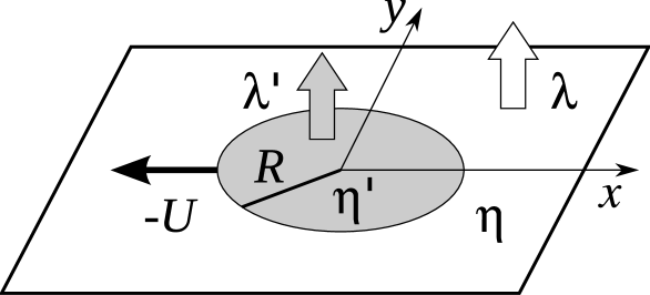
Figure 1: Schematic picture showing a section of an infinite membrane with viscosity $\eta$ and momentum decay parameter $\lambda$ in which a circular liquid domain of radius $R$ with viscosity $\eta^{\prime}$ and momentum decay parameter $\lambda^{\prime}$ is moving. The liquid domain moves with a velocity $-U$ in the $x$-direction.

The fluid velocity can generally be expressed as a gradient of some potential $\varphi$ and curl of some vector $\mathbf{A}=(0,0,A)$ which has only a single component lamb-75 . Then the velocities in the matrix and the domain regions are expressed as

$$\mathbf{v}=-\nabla\varphi+\nabla\times\mathbf{A},$$ (5)

and

$$\mathbf{v}^{\prime}=-\nabla\varphi^{\prime}+\nabla\times\mathbf{A}^{\prime},$$ (6)

respectively. Substituting eqs. (5) and (6) into eq. (4), we obtain

$$\nabla^{2}\varphi=0,~{}~{}~{}~{}~{}\nabla^{2}\varphi^{\prime}=0,$$ (7)

which are the Laplace equations. With the use of eqs. (5) and (6), one can show that eq. (3) can be satisfied if the pressures are given by

$$p=\lambda\varphi,~{}~{}~{}~{}~{}p^{\prime}=\lambda^{\prime}\varphi^{\prime},$$ (8)

while $A$ and $A^{\prime}$ obey the following equations:

$$(\nabla^{2}-\kappa^{2})A=0,~{}~{}~{}~{}~{}(\nabla^{2}-\kappa^{\prime 2})A^{\prime}=0.$$ (9)

Here we have defined the (inverse) hydrodynamic screening lengths for the matrix and the domain as $\kappa\equiv(\lambda/\eta)^{1/2}$ and $\kappa^{\prime}\equiv(\lambda^{\prime}/\eta^{\prime})^{1/2}$, respectively. We shall next seek for the solutions to eqs. (7) and (9) subject to the appropriate boundary conditions for the translational motion of the domain.

3 Calculation of drag coefficient

3.1 Velocity and stress tensor

It is convenient to work in the cylindrical polar coordinates $(r,\theta)$ with the origin at the center of the circular domain. First we consider the matrix region where $r>R$. Under the condition that the velocity and pressure must approach zero at large distances, we write down the solutions to eqs. (7) and (9) as follows:

$$\varphi=\frac{C_{1}}{r}\cos\theta,~{}~{}~{}~{}~{}A=C_{2}K_{1}(\kappa r)\sin\theta.$$ (10)

Here, $C_{1}$ and $C_{2}$ are unknown coefficients which will be determined from the boundary conditions, and $K_{1}(z)$ is the modified Bessel function of the second kind of order one. Although the general solutions for $\varphi$ and $A$ can be expressed as series expansions in terms of $r$, we have kept only the least number of terms satisfying the requisite pressure and velocity conditions. From eq. (5), the radial and tangential components of the velocity are given by

$$v_{r} =\left[\frac{C_{1}}{r^{2}}+\frac{C_{2}}{r}K_{1}(\kappa r)\right]\cos\theta,$$ (11)

$$v_{\theta} =\left[\frac{C_{1}}{r^{2}}+C_{2}\kappa K_{0}(\kappa r)+\frac{C_{2}}{r}K_{1}(\kappa r)\right]\sin\theta,$$ (12)

where we have used the recursion relations among the modified Bessel functions (see Appendix A). Then the components of the stress tensor can be obtained as

$$\sigma_{rr} =-p+2\eta\frac{\partial v_{r}}{\partial r}$$

$$=-\eta\left[C_{1}\left(\frac{\kappa^{2}}{r}+\frac{4}{r^{3}}\right)\right.$$

$$\left.+C_{2}\left(\frac{4}{r^{2}}K_{1}(\kappa r)+\frac{2\kappa}{r}K_{0}(\kappa r)\right)\right]\cos\theta,$$ (13)

$$\sigma_{r\theta} =\eta\left[\frac{1}{r}\frac{\partial v_{r}}{\partial\theta}+\frac{\partial v_{\theta}}{\partial r}-\frac{v_{\theta}}{r}\right]$$

$$=-\eta\left[\frac{4C_{1}}{r^{3}}\right.$$

$$\left.+C_{2}\left(\frac{4}{r^{2}}K_{1}(\kappa r)+\kappa^{2}K_{1}(\kappa r)+\frac{2\kappa}{r}K_{0}(\kappa r)\right)\right]\sin\theta.$$ (14)

Inside the liquid domain where $r<R$, the proper solutions to eqs. (7) and (9) subject to the condition that they do not diverge as $r\rightarrow 0$ are

$$\varphi^{\prime}=C_{1}^{\prime}r\cos\theta,~{}~{}~{}~{}~{}A^{\prime}=C_{2}^{\prime}I_{1}(\kappa^{\prime}r)\sin\theta,$$ (15)

Here, $C_{1}^{\prime}$ and $C_{2}^{\prime}$ are unknown coefficients, and $I_{1}(z)$ is the modified Bessel function of the first kind of order one. Since the corresponding radial and tangential components of the velocity are now

$$v^{\prime}_{r} =\left[-C_{1}^{\prime}+\frac{C_{2}^{\prime}}{r}I_{1}(\kappa^{\prime}r)\right]\cos\theta,$$ (16)

$$v^{\prime}_{\theta} =\left[C_{1}^{\prime}-C_{2}^{\prime}\kappa^{\prime}I_{0}(\kappa^{\prime}r)+\frac{C_{2}^{\prime}}{r}I_{1}(\kappa^{\prime}r)\right]\sin\theta,$$ (17)

the components of the stress tensor can be obtained as

$$\sigma^{\prime}_{rr} =-\eta^{\prime}\left[C_{1}^{\prime}\kappa^{\prime 2}r+C_{2}^{\prime}\left(\frac{4}{r^{2}}I_{1}(\kappa^{\prime}r)-\frac{2\kappa^{\prime}}{r}I_{0}(\kappa^{\prime}r)\right)\right]\cos\theta,$$ (18)

$$\sigma^{\prime}_{r\theta} =-\eta^{\prime}C_{2}^{\prime}\left[\frac{4}{r^{2}}I_{1}(\kappa^{\prime}r)+\kappa^{\prime 2}I_{1}(\kappa^{\prime}r)-\frac{2\kappa^{\prime}}{r}I_{0}(\kappa^{\prime}r)\right]\sin\theta.$$ (19)

3.2 Boundary conditions

Next we assume that the no-slip condition is satisfied at the domain boundary. This means that, at $r=R$, the radial component of the fluid velocities should be equal to the domain velocity $-U\cos\theta$, the tangential components should be continuous, and so should the components of the stress tensor landaulifshitz-flumech . These conditions are written as

$$v_{r} =-U\cos\theta,$$ (20)

$$v^{\prime}_{r} =-U\cos\theta,$$ (21)

$$v_{\theta} =v^{\prime}_{\theta},$$ (22)

$$\sigma_{r\theta} =\sigma^{\prime}_{r\theta}.$$ (23)

Since we have kept only the lowest order terms in $r$ for the solutions to eqs. (7) and (9) (see eqs. (10) and (15)), we are allowed to neglect the shape deformation of the circular domain while it moves. In other words, we are implicitly assuming that the line tension at the domain boundary exceeds a typical viscous force. A more quantitative argument to justify this condition will be given later.

Figure 2: The dimensionless drag coefficient $\zeta$ as a function of dimensionless domain radius $\epsilon=\kappa R$. The different curves are for $E=0.1$ (solid), $E=1$ (dashed), and $E=10$ (dotted).

Using the above four boundary conditions, we can obtain the four unknown coefficients $C_{1},C_{2},C_{1}^{\prime}$ and $C_{2}^{\prime}$ which are listed in Appendix B. In the following, we introduce the dimensionless parameters to measure the relative viscosities $E\equiv\eta/\eta^{\prime}$ and the relative decay parameters $L\equiv\lambda/\lambda^{\prime}$. We also use the notations $\epsilon\equiv\kappa R$ and $\epsilon^{\prime}\equiv\kappa^{\prime}R=\epsilon\sqrt{E/L}$ to measure the domain radius. Furthermore, the arguments of the modified Bessel functions will be omitted as $K_{n}\equiv K_{n}(\epsilon)$ and $I_{n}\equiv I_{n}(\epsilon^{\prime})$ in order to keep the notation compact.

3.3 Force exerted on a domain

The force exerted on the domain is given by the integral of the stress tensor over the boundary:

$$F=R\int_{0}^{2\pi}{\rm d}\theta\,(\sigma_{rr}\cos\theta-\sigma_{r\theta}\sin\theta).$$ (24)

After some calculation, the drag coefficient obtained from $\zeta=F/U$ becomes

$$\frac{\zeta(\epsilon;E,L)}{4\pi\eta}=\frac{\epsilon^{2}}{4}$$

$$+\frac{\epsilon K_{1}[(4+\epsilon^{\prime 2})I_{1}-2\epsilon^{\prime}I_{0}+2E(\epsilon^{\prime}I_{0}-2I_{1})]}{K_{0}[(4+\epsilon^{\prime 2})I_{1}-2\epsilon^{\prime}I_{0}]+E(2K_{0}+\epsilon K_{1})(\epsilon^{\prime}I_{0}-2I_{1})}.$$ (25)

An alternate form can be obtained by using the following recurrence relation

$$I_{0}(\epsilon^{\prime})=\frac{2I_{1}(\epsilon^{\prime})}{\epsilon^{\prime}}+I_{2}(\epsilon^{\prime}),$$ (26)

so that we have

$$\frac{\zeta(\epsilon;E,L)}{4\pi\eta}=\frac{\epsilon^{2}}{4}+\frac{\epsilon K_{1}(\epsilon^{\prime}I_{1}-2I_{2}+2EI_{2})}{K_{0}(\epsilon^{\prime}I_{1}-2I_{2})+E(2K_{0}+\epsilon K_{1})I_{2}}.$$ (27)

This is the main result of the paper.

Figure 3: The dimensionless drag coefficient $\zeta$ as a function of the relative viscosity ratio $E=\eta/\eta^{\prime}$ when $\epsilon=1$. The different curves are for $L=0.1$ (solid), $L=1$ (dashed) and $L=10$ (dotted).

In fig. 2, we plot the dimensionless drag coefficient $\zeta$ as a function of dimensionless domain size $\epsilon=\kappa R$ for $E=0.1,1,10$ when $L=1$. In all these cases, the drag coefficient increases with the domain radius $R$ as it should be. For fixed values of $\epsilon$, on the other hand, the drag coefficient is smaller when the domain viscosity $\eta^{\prime}$ becomes smaller (larger $E$). Fixing the domain size to $\epsilon=1$, we have plotted in figs. 3 and 4 the drag coefficient $\zeta$ as a function of $E$ and $L$, respectively. In the former, we chose various values of $L$ ranging from $L=0.1$ to $10$, while the values of $E$ were changed from $E=0.1$ to $10$ in the latter. Note that these graphs are both semi-log plots. From fig. 3, we see that the drag coefficient monotonically decreases with increasing $E$ (smaller domain viscosity). This can be attributed to the internal flows generated in the domain because they are more efficient in transporting the fluid around it. As a result, a domain with finite viscosity feels a smaller drag force than a rigid disk. The asymptotic values of $\zeta$ for $E\rightarrow 0$ and $E\rightarrow\infty$ converge to respective constants. In fig. 4, the drag coefficient is a decreasing function of $L$. The large $L$ values of $\zeta$ are dependent on $E$ as discussed below.

Figure 4: The dimensionless drag coefficient $\zeta$ as a function of the relative momentum decay parameter ratio $L=\lambda/\lambda^{\prime}$ when $\epsilon=1$. The different curves are for $E=0.1$ (solid), $E=1$ (dashed) and $E=10$ (dotted).

3.4 Limiting expressions

Next we examine several asymptotic limits of eq. (25) or eq. (27). Some useful formulae are listed in Appendix A.

First we consider arbitrary values of $E$ and $L$. In the limit of $\epsilon\rightarrow 0$, eq. (25) gives a logarithmic behavior,

$$\frac{\zeta(\epsilon\rightarrow 0)}{4\pi\eta}\approx\frac{1+E}{\ln{(2/\epsilon)}-\gamma+E[\ln{(2/\epsilon)}-\gamma+(1/2)]},$$ (28)

where $\gamma=0.5772\cdots$ is Euler’s constant. The above $E$-dependent logarithmic behavior is a new outcome of our result. In the opposite $\epsilon\rightarrow\infty$ limit, we have an algebraic dependence

$$\frac{\zeta(\epsilon\rightarrow\infty)}{4\pi\eta}\approx\frac{\epsilon^{2}}{4},$$ (29)

which does not depend on $E$. We also note that the above asymptotic expressions for small and large domain size limits do not depend on $L$.

Figure 5: The limiting dimensionless drag coefficient $\zeta_{0}$ (solid, eq. (30)) and $\zeta_{\infty}$ (dashed, eq. (31)) as a function of dimensionless domain radius $\epsilon=\kappa R$ when $L=1$.

For arbitrary $\epsilon$, we next consider the rigid disk case ($\eta^{\prime}\rightarrow\infty$) where the limit of $E\rightarrow 0$ is taken. Then we obtain

$$\frac{\zeta(\epsilon;E\rightarrow 0)}{4\pi\eta}=\frac{\epsilon^{2}}{4}+\frac{\epsilon K_{1}}{K_{0}}\equiv\frac{\zeta_{0}(\epsilon)}{4\pi\eta},$$ (30)

which coincides with the result by Evans and Sackmann evans-88 . The opposite limit of $E\rightarrow\infty$ corresponds to a 2D gas bubble ($\eta^{\prime}\rightarrow 0$). In this case, we obtain a different expression:

$$\frac{\zeta(\epsilon;E\rightarrow\infty)}{4\pi\eta}=\frac{\epsilon^{2}}{4}+\frac{2\epsilon K_{1}}{2K_{0}+\epsilon K_{1}}\equiv\frac{\zeta_{\infty}(\epsilon)}{4\pi\eta}.$$ (31)

In fig. 5, we plot both $\zeta_{0}$ and $\zeta_{\infty}$ as a function of $\epsilon$ in log-log scales. In the limit of $\epsilon\rightarrow\infty$, the difference between the two curves is the order of $\epsilon$ which becomes negligibly small compared to the first terms in eqs. (30) and (31). Upon taking the $\epsilon\rightarrow 0$ limit of eqs. (30) and (31), we obtain

$$\frac{\zeta_{0}(\epsilon\rightarrow 0)}{4\pi\eta}\approx\frac{1}{\ln{(2/\epsilon)}-\gamma},$$ (32)

$$\frac{\zeta_{\infty}(\epsilon\rightarrow 0)}{4\pi\eta}\approx\frac{1}{\ln{(2/\epsilon)}-\gamma+(1/2)}.$$ (33)

These are nothing but the $E\rightarrow 0$ and $E\rightarrow\infty$ limits of eq. (28). We note that small $\epsilon$ behavior of $\zeta_{0}$ and $\zeta_{\infty}$ do not coincide in fig. 5. The limiting expressions of eqs. (30) and (31) for $\epsilon\rightarrow\infty$ coincide with eq. (29).

In the limit of $L\rightarrow 0$, which is the case of high momentum dissipation in the domain region, we recover eq. (30) again;

$$\frac{\zeta(\epsilon;L\rightarrow 0)}{4\pi\eta}=\frac{\epsilon^{2}}{4}+\frac{\epsilon K_{1}}{K_{0}}.$$ (34)

In the opposite $L\rightarrow\infty$ limit, we obtain

$$\frac{\zeta(\epsilon;L\rightarrow\infty)}{4\pi\eta}=\frac{\epsilon^{2}}{4}+\frac{2\epsilon(1+E)K_{1}}{2(1+E)K_{0}+\epsilon EK_{1}}.$$ (35)

which depends on $E$ as observed in fig. 4. Equation (35) reduces to eqs. (30) and (31) for $E\rightarrow 0$ and $E\rightarrow\infty$, respectively.

4 Conclusion and discussion

In summary, we have obtained the drag coefficient of a circular liquid domain which has a finite viscosity using a 2D hydrodynamic equation with momentum decay or the 2D Brinkman equation. We showed that the drag coefficient decreases as the domain viscosity becomes smaller with respect to the matrix viscosity. This is because the flow in the domain helps to transport the fluid in the surrounding matrix more efficiently. Our result shows an $E$-dependence in the small domain size limit (eq. (28)). New limiting expressions for the $E\rightarrow\infty$ (eq. (31)) and $L\rightarrow\infty$ (eq. (35)) are also obtained.

Several points merit further discussion. We first discuss the realistic value of $E=\eta/\eta^{\prime}$ in the case of lipid domains. Lipid domains are known to arise from a phase separation between a liquid-ordered ($L_{\rm o}$) phase rich in saturated lipid such as sphingomyelin and a liquid-disordered ($L_{\rm d}$) phase rich in unsaturated lipid veatch-05 . Applying the pulsed field gradient NMR spectroscopy, Orädd et al. measured lateral diffusion coefficients of a single lipid molecule both in the $L_{\rm o}$ and $L_{\rm d}$ phases oradd-05 . With the use of the SD logarithmic expression for the diffusion coefficient, the 2D viscosities of these phases are estimated as $\eta_{\rm o}\approx 1.6\times 10^{-9}$ Ns/m and $\eta_{\rm d}\approx 0.4\times 10^{-9}$ Ns/m at 293 K (the membrane thickness is chosen to be $h\approx 3.8\times 10^{-9}$ m). When the $L_{\rm o}$ phase forms a domain in the matrix of the $L_{\rm d}$ phase, the typical viscosity ratio would be $E\approx 0.2$. In the opposite case where the $L_{\rm d}$ phase forms a domain, the ratio tends to be $E\approx 4$. Hence, it is necessary to take into account the finite viscosity ratio between the domain and the matrix rather than regarding the domain as a rigid disk. Incidentally, sphingomyelin constituting the $L_{\rm o}$ phases has a large head group which can protrude out into the 3D fluid, whereas the $L_{\rm d}$ phase are devoid of such structures simons-97 . It is therefore reasonable to assume that the momentum decay parameter $\lambda$ experienced by the $L_{\rm o}$ and $L_{\rm d}$ domains are different.

When imposing the boundary conditions as given from eq. (20) to (23), we have assumed that the domain does not undergo any shape deformation. This implies that the line tension should be large enough to overcome the viscous force of deformation. In the case of lipid domains, the line tension was measured to be $\sigma\sim 10^{-12}$ N using domain boundary flicker spectroscopy esposito-07 . For a flow of the order of $U\sim 10^{-6}$ m/s, a typical viscous force turns out be $\eta U\sim 10^{-15}$ N which is much smaller than $\sigma$. Hence it is reasonable to assume that the line tension is large enough to maintain the circular shape of the domains unless the temperature is very close to the critical point. Different boundary conditions were used in order to consider the relaxation of deformed domains in a polymer monolayer mann-95 .

The crossover from the logarithmic to algebraic behaviors of the drag coefficient takes place when $\epsilon\sim 1$ or $R\sim\kappa^{-1}$. A typical domain size which corresponds to this condition is roughly estimated below. As stated in sect. 2, the momentum decay parameter for a supported membrane was originally identified as $\lambda=\eta_{\rm f}/H$, where $\eta_{\rm f}$ is the 3D viscosity in the outer fluid and $H$ is the thickness of a thin lubricating water which exists between the membrane and substrate evans-88 . In this situation, we have the hydrodynamic screening length $\kappa^{-1}=\sqrt{\eta H/\eta_{\rm f}}$. Although we do not assume the presence of a solid substrate, the hydrodynamic screening length in the Brinkman approach would typically be $\kappa^{-1}\sim 10^{-7}$ m when $H=10^{-8}$ m, $\eta_{\rm f}\sim 10^{-3}$ Ns/m² and $\eta\sim 10^{-9}$ Ns/m. Domain size in the order of $R\sim 10^{-7}$ m is accessible in the experiments.

Within the present Brinkman model, the drag coefficient has a $R^{2}$ dependence in the large size limit as in eq. (29). Such a behavior was indeed observed experimentally for Brownian motion of phase-separated domains on stacked-supported membranes kaizuka-04 . However, this dependence differs from the asymptotic analysis of the SD model according to which the drag coefficient increases linearly with $R$ (similar to a 3D sphere) hughes-81 . For ternary vesicles, Cicuta et al. have measured the drag coefficient of a domain which is proportional to $R$ cicuta-07 , supporting the SD model. The large scale behavior of the Brinkman model and the SD model differs because the former is essentially a 2D model while the latter has a 3D character. It should be also noted that the hydrodynamic screening length in the SD theory is given by $\nu^{-1}\equiv\eta/\eta_{\rm f}$ which is different from $\kappa^{-1}$. In the present Brinkman approach, the hydrodynamic screening length is the geometric mean of $\nu^{-1}$ and $H$.

At this stage we mention that, based on the SD theory, an integral form of the drag coefficient for a 2D liquid domain with $E=1$ was obtained by De Koker as dekoker-02

$$\frac{\zeta_{\rm DK}}{4\pi\eta}=\frac{1}{4}\left[\int_{0}^{\infty}{\rm d}z\,\frac{J_{1}^{2}(z)}{z^{2}(z+\delta)}\right]^{-1},$$ (36)

where $\delta\equiv\nu R$ and $J_{1}(z)$ is the Bessel function of the first kind. We have estimated the above integral numerically. In the limit of $\delta\rightarrow 0$, the above expression gives a logarithmic dependence on $R$, in agreement with our result for small $\epsilon$ as seen in eq. (28). In the opposite limit of $\delta\rightarrow\infty$, however, $\zeta_{\rm DK}$ is proportional to $R$ due to the 3D nature of the SD theory. As describe above, this is different from eq. (29) which gives the $R^{2}$ dependence.

Several authors considered a more general scenario in which a disk or a domain moves in a membrane being located at a finite distance $H$ from a fixed substrate lubensky-96 ; stone-98 ; fischer-04 ; Tserkovnyak-06 ; inaura-08 . Among these, Stone and Ajdari numerically solved the coupled dual integral equations which are obtained as solutions for the Stokes equations stone-98 . They showed that the Brinkman model gives a qualitatively good approximation over a wide range of membrane-substrate separations. One can explicitly show that the Brinkman and the SD models are recovered in the limit of $H\rightarrow 0$ and $H\rightarrow\infty$, respectively.

For comparison, we finally write down the analogous expression for the drag coefficient of a spherical drop having 3D viscosity $\eta^{\prime}_{3}$ and radius $R$ moving in a fluid of 3D viscosity $\eta_{3}$ rybczynski-11 ; hadamard-11 ; landaulifshitz-flumech

$$\frac{\zeta_{3}}{2\pi\eta_{3}R}=\frac{2E_{3}+3}{E_{3}+1},$$ (37)

where $E_{3}=\eta_{3}/\eta^{\prime}_{3}$. In the solid sphere limit ($\eta^{\prime}_{3}\rightarrow\infty$), we obtain $\zeta_{3}=6\pi\eta_{3}R$ (the Stokes result). In the opposite bubble limit ($\eta^{\prime}_{3}\rightarrow 0$), we have $\zeta_{3}=4\pi\eta_{3}R$. The reduction in the drag coefficient with the decrease in the drop viscosity $\eta^{\prime}_{3}$ is similar to that seen for a liquid domain in 2D as discussed before. It is also important to point out that the effect of viscosity ratio $E_{3}$ exists for all the drop sizes $R$ because there is no typical length scale for a 3D fluid. This is in sharp contrast to our model in which the hydrodynamic screening length $\kappa^{-1}$ plays a crucial role.

We thank S. L. Keller and Y. Sakuma for useful discussions. This work was supported by KAKENHI (Grant-in-Aid for Scientific Research) on Priority Area “Soft Matter Physics” and Grant No. 21540420 from the Ministry of Education, Culture, Sports, Science and Technology of Japan.

Appendix A. Useful formulae

According to ref. abram-stegun , the following recursion relations hold:

$$K_{0}^{\prime}(z) =-K_{1}(z),$$ (A.1)

$$K_{1}^{\prime}(z) =-K_{0}(z)-\frac{K_{1}(z)}{z},$$ (A.2)

$$I_{0}^{\prime}(z) =I_{1}(z),$$ (A.3)

$$I_{1}^{\prime}(z) =I_{0}(z)-\frac{I_{1}(z)}{z}.$$ (A.4)

Here the primes indicate the derivative with respect to $z$.

In the limit of $z\rightarrow 0$, we have

$$K_{0}(z) \approx\ln\left(\frac{2}{z}\right)-\gamma+\frac{1}{4}\left[1+\ln\left(\frac{2}{z}\right)-\gamma\right]z^{2}+\cdots,$$ (A.5)

$$K_{1}(z) \approx\frac{1}{z}-\frac{1}{2}\left[\frac{1}{2}+\ln\left(\frac{2}{z}\right)-\gamma\right]z+\cdots,$$ (A.6)

$$I_{0}(z) \approx 1+\frac{z^{2}}{4}+\cdots,$$ (A.7)

$$I_{1}(z) \approx\frac{z}{2}+\frac{z^{3}}{16}+\cdots,$$ (A.8)

$$I_{2}(z) \approx\frac{z^{2}}{8}+\frac{z^{4}}{96}+\cdots,$$ (A.9)

where $\gamma=0.5772\ldots$ is the Euler constant. In the limit of $z\rightarrow\infty$, we have

$$K_{n}(z) \approx\sqrt{\frac{\pi}{2z}}e^{-z}\left[1+\frac{4n^{2}-1}{8z}+\cdots\right],$$ (A.10)

$$I_{n}(z) \approx\frac{e^{z}}{\sqrt{2\pi z}}\left[1-\frac{4n^{2}-1}{8z}+\cdots\right].$$ (A.11)

Appendix B. Coefficients $C_{1},C_{2},C_{1}^{\prime}$ and $C_{2}^{\prime}$

The coefficients $C_{1},C_{2},C_{1}^{\prime}$ and $C_{2}^{\prime}$ are given by

$$C_{1} =-R^{2}U-2K_{1}RU/(\kappa K_{0})$$

$$+2K_{1}^{2}R^{2}\eta U(-2I_{1}+I_{0}R\kappa^{\prime})/[K_{0}(M_{1}+M_{2})],$$ (B.1)

$$C_{2} =4I_{0}R(\eta-\eta^{\prime})\kappa^{\prime}U/[\kappa(M_{1}+M_{2})]$$

$$-2I_{1}U[4\eta-\eta^{\prime}(4+R^{2}\kappa^{\prime 2})]/[\kappa(M_{1}+M_{2})],$$ (B.2)

$$C_{1}^{\prime} =U+2I_{1}K_{1}R\eta\kappa U/(M_{1}+M_{2}),$$ (B.3)

$$C_{2}^{\prime} =2K_{1}R^{2}\eta\kappa U/(M_{1}+M_{2}),$$ (B.4)

with

$$M_{1} =2I_{0}K_{0}R(\eta-\eta^{\prime})\kappa^{\prime}+I_{0}K_{1}R^{2}\eta\kappa\kappa^{\prime},$$ (B.5)

$$M_{2} =-2I_{1}K_{1}R\eta\kappa-4I_{1}K_{0}\eta+I_{1}K_{0}\eta^{\prime}(4+R^{2}\kappa^{\prime 2}).$$ (B.6)

In the above, $K_{n}=K_{n}(\kappa R)=K_{n}(\epsilon)$ and $I_{n}=I_{n}(\kappa^{\prime}R)=I_{n}(\epsilon^{\prime})$ as denoted in the text.

References

- (1) R. Peters, R.J. Cherry, Proc. Natl. Acad. Sci. USA 79, 4317 (1982).
- (2) J. Lippincott-Schwartz, E. Snapp, A. Kenworthy, Nat. Rev. Mol. Cell Biol. 2, 444 (2001).
- (3) M. Vrljic, Y. Nishimura, S. Brasselet, W.E. Moerner, H.M. McConnell, Biophys. J. 83, 2681 (2002).
- (4) E.A.J. Reitz, J.J. Neefjes, Nat. Cell Biol. 3, E145 (2001).
- (5) Y. Gambin, R. Lopez-Esparza, M. Reffay, E. Sierecki, N.S. Gov, M. Genest, R.S. Hodges, W. Urbach, Proc. Natl. Acad. Sci. USA 103, 2098 (2007).
- (6) J.F. Klingler, H.M. McConnell, J. Phys. Chem. 97, 6096 (1993).
- (7) G. Orädd, P.W. Westerman, G. Lindblom, Biophys. J. 89, 315 (2005).
- (8) P. Cicuta, S.L. Keller, S.L. Veatch, J. Phys. Chem. B 111, 3328 (2007).
- (9) M. Yanagisawa, M. Imai, T. Masui, S. Komura, T. Ohta, Biophys. J. 92, 115 (2007).
- (10) Y. Sakuma, N. Urakami, Y. Ogata, M. Nagao, S. Komura, T. Kawakatsu, M. Imai, preprint.
- (11) S.L. Veatch, S.L. Keller, Biochim. Biophys. Acta 1746, 172 (2005).
- (12) K. Simons, E. Ikonen, Nature 387, 569 (1997).
- (13) P.G. Saffman, M. Delbrück, Proc. Natl. Acad. Sci. USA 72, 3111 (1975).
- (14) P.G. Saffman, J. Fluid Mech. 73, 593 (1976).
- (15) B.D. Hughes, B.A. Pailthorpe, L.R. White, J. Fluid Mech. 110, 349 (1981).
- (16) A.J. Levine, F.C. MacKintosh, Phys. Rev. E 66, 061606 (2002).
- (17) A.J. Levine, T.B. Liverpool, F.C. MacKintosh, Phys. Rev. Lett. 93, 038102 (2004).
- (18) A.J. Levine, T.B. Liverpool, F.C. MacKintosh, Phys. Rev. E 69, 021503 (2004).
- (19) E. Evans, E. Sackmann, J. Fluid Mech. 194, 553 (1988).
- (20) T. Izuyama, Dynamics of ordering processes in condensed matter, edited by S. Komura and H. Furukawa (Plenum, New York, 1988).
- (21) H.C. Brinkman, Appl. Sci. Res. A 1, 27 (1947).
- (22) B. Alberts, A. Johnson, P. Walter, J. Lewis, M. Raff, Molecular Biology of the Cell (Garland Science, New York, 2008).
- (23) W. Rybczyski, Bull. Acad. Sci. Cracovie Ser. A 40, 40 (1911).
- (24) J.S. Hadamard, Compt. Rend. Acad. Sci. (Paris) 152, 1735 (1911).
- (25) H.A. Stone, H.M. McConnell, Proc. R. Soc. Lond. A 448, 97 (1995).
- (26) D.K. Lubensky, R.E. Goldstein, Phys. Fluids 8, 843 (1996).
- (27) J.C. Alexander, A.J. Bernoff, E.K. Mann, J.A. Mann Jr, J.R. Wintersmith, L. Zou, J. Fluid Mech. 571, 191 (2006).
- (28) Owing to the reviewer’s comment, we recently came to know that, based on the SD theory, De Koker obtained an integral form of the drag force of a liquid domain which has the same viscosity as that of the matrix. Although this result was not published, we will compare it with our result in sect. 4.
- (29) L.D. Landau, E.M. Lifshitz, Fluid mechanics (Pergamon Press, Oxford, 1987).
- (30) H. Lamb, Hydrodynamics (Cambridge University Press, New York, 1975).
- (31) K. Seki, S. Komura, Phys. Rev. E 47, 2377 (1993).
- (32) S. Komura, K. Seki, J. Physique II 5, 5 (1995).
- (33) K. Seki, S. Komura, M. Imai, J. Phys.: Condens. Matter 19, 072101 (2007).
- (34) N. Oppenheimer, H. Diamant, Biophys. J. 96, 3041 (2009).
- (35) C. Esposito, A. Tian, S. Melamed, C. Johnson, S.Y. Tee, T. Baumgart, Biophys. J. 93, 3169 (2007).
- (36) E.K. Mann, S. Hénon, D. Langevin, J. Meunier, L. Léger, Phys. Rev. E 51, 5708 (1995).
- (37) Y. Kaizuka, J.T. Groves, Biophys. J. 86, 905 (2004).
- (38) S. Wurlitzer, H. Schmiedel and Th.M. Fischer, Langmuir. 18, 4393 (2002)
- (39) H. Stone, A. Ajdari, J. Fluid Mech. 369, 151 (1998).
- (40) T.M. Fischer, J. Fluid Mech. 498, 123 (2004).
- (41) Y. Tserkovnyak, D.R. Nelson, Proc. Natl. Acad. Sci. USA 103, 15002 (2006).
- (42) K. Inaura, Y. Fujitani, J. Phys. Soc. Jpn. 77, 114603 (2008).
- (43) M. Abramowitz, I.A. Stegun, Handbook of mathematical functions (Dover, New York, 1972).