Hot Plasma Waves in Schwarzschild Magnetosphere

Abstract

In this paper we examine the wave properties of hot plasma living in Schwarzschild magnetosphere. The 3+1 GRMHD perturbation equations are formulated for this scenario. These equations are Fourier analyzed and then solved numerically to obtain the dispersion relations for non-rotating, rotating non-magnetized and rotating magnetized plasma. The wave vector is evaluated which is used to calculate refractive index. These quantities are shown in graphs which are helpful to discuss the dispersive properties of the medium near the event horizon.

Keywords: 3+1 formalism, GRMHD equations, hot plasma, magnetosphere, dispersion relations.
Keywords: 95.30.Sf; 95.30.Qd, 04.30.Nk

1 Introduction

In general relativity (GR), the term black hole evokes the mysterious gravity. Black holes are among the most remarkable predictions of GR, which are a reality today. These are usually found in X-ray binaries and in the centers of galaxies. The existence of rotating stars indicates their rotational behavior. A rotating black hole gradually reduces to a Schwarzschild (non-rotating) black hole by the extraction of its rotating energy. Plasmas are abundant in nature. More than $99\%$ of all known matter is in the plasma state. All the stars are made of plasma, and even the space between the stars is filled with plasma. Commonly space plasma occurs in a hot state. The strong gravity of the black hole strips the plasma from the surrounding star. Thus the plasma gathered around the black hole in the form of accretion disk. The moving plasma creates a magnetic field. The region surrounding the black hole admitting the magnetic field is known as magnetosphere. The theory of general relativistic magnetohydrodynamics (GRMHD) is probably the most accurate approach to investigate the dynamics of relativistic, magnetized plasma.

The Schwarzschild black hole is non-rotating and hence the magnetospheric plasma falls freely along radial direction only. Perturbations in the Schwarzschild regime, either geometrical or physical, have always been of interest by the relativists. Regge and Wheeler [1], Zerilli [2] and Price [3] discussed the gravitational perturbations. Fiziev [4] presented the exact solution of Regge-Wheeler equations. These equations describe the axial perturbations of the Schwarzschild metric in linear approximation. The quasi-static problem of electric field in the Schwarzschild black hole was solved by Hanni and Ruffini [5]. Sakai and Kawata [6] developed a special relativistic approach for a linearized treatment of plasma waves in the Schwarzschild black hole magnetosphere.

In general relativity, a 3+1 hypersurface split of spacetime is appropriate to understand the black hole physics. This split was developed by Arnowitt, Deser and Misner (ADM) [7] to study the quantization of gravitational field. The formalism has wide applications in numerical relativity. The 3+1 approach has been used by many authors [8]-[10] to discuss different features in GR. Thorne and Macdonald [11]-[12] developed the electromagnetic theory in black hole regime using this formalism. Holcomb and Tajima [13], Holcomb [14] and Dettmann et al. [15] studied some properties of wave propagation for the Friedmann universe. Buzzi et al. [16] investigated relativistic two fluid plasma wave properties in the vicinity of the Schwarzschild black hole. Ali and Rahman [17] adopted the technique used by Buzzi et al. [16] to analyze the transverse electromagnetic waves propagating in a plasma close to the Schwarzschild-de Sitter black hole. Zhang [18] formulated the black hole theory for stationary symmetric GRMHD. He [19] also discussed the behavior of cold plasma perturbations in the Kerr magnetosphere. Sharif et al. [20]-[24] discussed properties of plasma waves by using real and complex wave numbers. The analysis was given both for cold and isothermal plasmas.

A lot of work has been done using cold and isothermal plasma but no one has used hot plasma in this context which is the basic constituent of nature. This is the most general plasma which reduces to cold and isothermal plasma with some restrictions. We have considered this plasma around the black hole to check the possibility of receiving information. This work focusses on the investigation of hot plasma wave properties in the Schwarzschild magnetosphere. We shall apply perturbation and Fourier analysis techniques. The dispersion relations are calculated with the help of the software Mathematica to obtain the wave vector. This will be used to evaluate the refractive index and its change with respect to angular frequency. The wave properties will be found through these quantities.

The outline of the paper is as follows. In Section 2, we shall provide the general line element and restrict it to the Schwarzschild planar analogue. Section 3 includes the plasma assumptions for perturbation and Fourier analysis. Moreover, the perturbed and Fourier analyzed 3+1 GRMHD equations are specified for hot plasma. In Sections 4, 5 and 6, we restrict these equations to non-rotating, rotating non-magnetized and rotating magnetized plasmas and discuss the wave properties. Section 7 contains summary of the results.

2 3+1 Split of Spacetime

In ADM 3+1 split, the four dimensional spacetime is decomposed into a succession of three dimensional spacelike hypersurfaces with the directions normal to them taken to be universal time direction. The line element of spacetime in 3+1 formalism can be written as [19]

$$ds^{2}=-\alpha^{2}dt^{2}+\gamma_{ij}(dx^{i}+\beta^{i}dt)(dx^{j}+\beta^{j}dt),$$ (2.1)

where $\alpha$ is the lapse function which describes the ratio of fiducial proper time to universal time, i.e., $\alpha=\frac{d\tau}{dt}$. The shift vector components $\beta^{i}$ indicate the shift of spatial coordinates as one moves from one hypersurface to next. $\gamma_{ij}$ are components of three dimensional hypersurface (the absolute space) metric. A natural observer is associated with this spacetime, called the fiducial observer (FIDO).

The Schwarzschild black hole is non-rotating, thus in the planar analogue of Schwarzschild geometry, the shift $\beta$ vanishes and the above line element becomes [22]

$$ds^{2}=-\alpha^{2}(z)dt^{2}+dx^{2}+dy^{2}+dz^{2}.$$ (2.2)

Here, the directions $z$, $x$ and $y$ are analogous to Schwarzschild’s $r$, $\phi$ and $\theta$ respectively.

3 3+1 GRMHD Equations with Relative Assumptions

For the plasma existing in the general and Scwarzschild planar analogues (given by Eqs.(2.1) and (2.2)), the 3+1 GRMHD equations are given in Appendix A. We assume that hot plasma surrounds the Schwarzschild black hole. The specific enthalpy of the fluid is [19]

$$\mu=\frac{\rho+p}{\rho_{0}},$$ (3.1)

where $\rho_{0},~{}\rho$ and $p$ denote the rest-mass density, moving mass density and pressure respectively. Equation (3.1) indicates the exchange of heat between the plasma and the magnetic field of the fluid.

We can modify the 3+1 GRMHD equations given by Eqs.(A6)-(Appendix A) for hot plasma living in the Schwarzschild spacetime as follows

$$\frac{\partial\textbf{B}}{\partial t}=\nabla\times(\alpha\textbf{V}\times\textbf{B}),$$ (3.2)

$$\nabla.\textbf{B}=0,$$ (3.3)

$$\frac{\partial(\rho+p)}{\partial t}+(\rho+p)\gamma^{2}\textbf{V}.\frac{\partial\textbf{V}}{\partial t}+(\rho+p)\gamma^{2}V.(\alpha\textbf{V}.\nabla)\textbf{V}$$

$$+(\rho+p)\nabla.(\alpha\textbf{V})=0,$$ (3.4)

$$\left\{\left((\rho+p)\gamma^{2}+\frac{\textbf{B}^{2}}{4\pi}\right)\delta_{ij}+(\rho+p)\gamma^{4}V_{i}V_{j}-\frac{1}{4\pi}B_{i}B_{j}\right\}\left(\frac{1}{\alpha}\frac{\partial}{\partial t}\right.$$

$$\left.+\textbf{V}.\nabla\right)V^{j}+\gamma^{2}V_{i}(\textbf{V}.\nabla)(\rho+p)-\left(\frac{\textbf{B}^{2}}{4\pi}\delta_{ij}-\frac{1}{4\pi}B_{i}B_{j}\right)V^{j}_{,k}V^{k}$$

$$=-(\rho+p)\gamma^{2}a_{i}-p_{,i}+\frac{1}{4\pi}(\textbf{V}\times\textbf{B})_{i}\nabla.(\textbf{V}\times\textbf{B})-\frac{1}{8\pi\alpha^{2}}(\alpha\textbf{B})^{2}_{,i}$$

$$+\frac{1}{4\pi\alpha}(\alpha B_{i})_{,j}B^{j}-\frac{1}{4\pi\alpha}[\textbf{B}\times\{\textbf{V}\times(\nabla\times(\alpha\textbf{V}\times\textbf{B}))\}]_{i},$$ (3.5)

$$\frac{1}{\alpha}\frac{\partial}{\partial t}\{(\rho+p)\gamma^{2}-p\}+(\rho+p)\gamma^{2}\textbf{V}.\textbf{a}+(\rho+p)\gamma^{4}\textbf{V}.(\textbf{V}.\nabla)\textbf{V}$$

$$-\frac{1}{2\pi}\textbf{a}.\{(\textbf{V}\times\textbf{B})\times\textbf{B}\}=\frac{1}{4\pi}\textbf{B}.\{\nabla\times(\textbf{V}\times\textbf{B})\}$$

$$-\frac{1}{4\pi}\left\{2\frac{1}{\alpha}(\textbf{V}\times\textbf{B}).\frac{\partial}{\partial t}(\textbf{V}\times\textbf{B})+(\textbf{V}\times\textbf{B}).(\textbf{a}\times\textbf{B})\right.$$

$$\left.+\textbf{B}.\frac{1}{\alpha}\frac{\partial\textbf{B}}{\partial t}\right\},$$ (3.6)

where B and V are the velocity and magnetic field of the fluid as measured by the FIDO.

We consider rotating background (plasma is rotating), plasma is not only moving along radial direction but it rotates as well. Due to its rotation, wave propagates along axial direction also and thus propagates in $(x,z)$-plane. It is assumed that the FIDO measured velocity of fluid and magnetic field lie in $xz$-plane

$$\textbf{V}=V(z)\textbf{e}_{x}+u(z)\textbf{e}_{z},\quad\textbf{B}=B[\lambda(z)\textbf{e}_{x}+\textbf{e}_{z}],$$ (3.7)

where $B$ is an arbitrary constant. Here $\lambda$, $u$ and $V$ are related by [20]

$$V=\frac{V^{F}}{\alpha}+\lambda u,$$ (3.8)

where $V^{F}$ is an integration constant. The Lorentz factor $\gamma=\frac{1}{\sqrt{1-\textbf{V}^{2}}}$ takes the following form

$$\gamma=\frac{1}{\sqrt{1-u^{2}-V^{2}}}.$$ (3.9)

The plasma flow in the magnetosphere can be characterized by its density $\rho$, pressure $p$, velocity V and magnetic field B. When the flow is perturbed, these variables will become

$$\rho=\rho^{0}+\delta\rho=\rho^{0}+\rho\widetilde{\rho},\quad p=p^{0}+\delta p=p^{0}+p\widetilde{p},$$

$$\textbf{V}=\textbf{V}^{0}+\delta\textbf{V}=\textbf{V}^{0}+\textbf{v},\quad\textbf{B}=\textbf{B}^{0}+\delta\textbf{B}=\textbf{B}^{0}+B\textbf{b},$$ (3.10)

where $\rho^{0},~{}p^{0},~{}\textbf{V}^{0}$ and $\textbf{B}^{0}$ are unperturbed quantities. The linear perturbations in these quantities are denoted by $\delta\rho$, $\delta p$, $\delta\textbf{V}$ and $\delta\textbf{B}$ respectively.

We shall use the following dimensionless notations for the perturbed quantities

$$\tilde{\rho}=\tilde{\rho}(t,z),\quad\tilde{p}=\tilde{p}(t,z),$$

$$\textbf{v}=\delta\textbf{V}=v_{x}(t,z)\textbf{e}_{x}+v_{z}(t,z)\textbf{e}_{z},$$

$$\textbf{b}=\frac{\delta\textbf{B}}{B}=b_{x}(t,z)\textbf{e}_{x}+b_{z}(t,z)\textbf{e}_{z},$$ (3.11)

where $\widetilde{\rho},~{}\widetilde{p},v_{x},v_{z},b_{x}$ and $b_{z}$ are dimensionless quantities. For Fourier analysis, we assume the harmonic space and time dependence of perturbations

$$\widetilde{\rho}(t,z)=c_{1}e^{-\iota(\omega t-kz)}, \widetilde{p}(t,z)=c_{2}e^{-\iota(\omega t-kz)},$$

$$v_{z}(t,z)=c_{3}e^{-\iota(\omega t-kz)}, v_{x}(t,z)=c_{4}e^{-\iota(\omega t-kz)},$$

$$b_{z}(t,z)=c_{5}e^{-\iota(\omega t-kz)}, b_{x}(t,z)=c_{6}e^{-\iota(\omega t-kz)},$$ (3.12)

where $k$ is $z$-component of the wave vector $(0,0,k)$ and $\omega$ is the angular frequency. We can use the wave vector to obtain the refractive index which we shall use to deduce the plasma wave properties. We define the wave vector and the refractive index as follows:

• Wave Vector: A wave vector is a vector which points in the direction of propagation of wave. Its magnitude gives the wave number.

• Refractive Index: It is the ratio of the speed of light in vacuum to the speed of light in the other medium [25]. If the refractive index is greater than one and its change with respect to angular frequency is positive, the dispersion is said to be normal, otherwise anomalous.

When we introduce linear perturbations from Eq.(3), the perfect GRMHD Eqs.(3.2)-(3) turn out to be

$$\frac{\partial(\delta\textbf{B})}{\partial t}=\nabla\times(\alpha\textbf{v}\times\textbf{B})+\nabla\times(\alpha\textbf{V}\times\delta\textbf{B}),$$ (3.13)

$$\nabla.(\delta\textbf{B})=0,$$ (3.14)

$$\frac{1}{\alpha}\frac{\partial(\delta\rho+\delta p)}{\partial t}+(\rho+p)\gamma^{2}\textbf{V}.(\frac{1}{\alpha}\frac{\partial}{\partial t}+\textbf{V}.\nabla)\textbf{v}+(\rho+p)(\nabla.\textbf{v})$$

$$=-2(\rho+p)\gamma^{2}(\textbf{V}.\textbf{v})(\textbf{V}.\nabla)\ln\gamma-(\rho+p)\gamma^{2}(\textbf{V}.\nabla\textbf{V}).\textbf{v}$$

$$+(\rho+p)(\textbf{v}.\nabla\ln u),$$ (3.15)

$$\left\{\left((\rho+p)\gamma^{2}+\frac{\textbf{B}^{2}}{4\pi}\right)\delta_{ij}+(\rho+p)\gamma^{4}V_{i}V_{j}-\frac{1}{4\pi}B_{i}B_{j}\right\}\frac{1}{\alpha}\frac{\partial v^{j}}{\partial t}$$

$$+\frac{1}{4\pi}[\textbf{B}\times\{\textbf{V}\times\frac{1}{\alpha}\frac{\partial(\delta\textbf{B})}{\partial t}\}]_{i}+(\rho+p)\gamma^{2}v_{i,j}V^{j}+(\rho+p)$$

$$\times\gamma^{4}V_{i}v_{j,k}V^{j}V^{k}+\gamma^{2}V_{i}(\textbf{V}.\nabla)(\delta\rho+\delta p)+\gamma^{2}V_{i}(\textbf{v}.\nabla)(\rho+p)$$

$$+\gamma^{2}v_{i}(\textbf{V}.\nabla)(\rho+p)+\gamma^{4}(2\textbf{V}.\textbf{v})V_{i}(\textbf{V}.\nabla)(\rho+p)-\frac{1}{4\pi\alpha}\{(\alpha\delta B_{i})_{,j}$$

$$-(\alpha\delta B_{j})_{,i}\}B^{j}=-(\delta p)_{i}-\gamma^{2}\{(\delta\rho+\delta p)+2(\rho+p)\gamma^{2}(\textbf{V}.\textbf{v})\}a_{i}$$

$$+\frac{1}{4\pi\alpha}\{(\alpha B_{i})_{,j}-(\alpha B_{j})_{,i}\}\delta B^{j}-(\rho+p)\gamma^{4}(v_{i}V^{j}+v^{j}V_{i})V_{k,j}V^{k}$$

$$-\gamma^{2}\{(\delta\rho+\delta p)V^{j}+2(\rho+p)\gamma^{2}(\textbf{V}.\textbf{v})V^{j}+(\rho+p)v^{j}\}V_{i,j}$$

$$-\gamma^{4}V_{i}\{(\delta\rho+\delta p)V^{j}+4(\rho+p)\gamma^{2}(\textbf{V}.\textbf{v})V^{j}$$

$$+(\rho+p)v^{j}\}V_{j,k}V^{k},$$ (3.16)

$$\gamma^{2}\frac{1}{\alpha}\frac{\partial(\delta\rho+\delta p)}{\partial t}+\frac{2}{\alpha}(\rho+p)\gamma^{4}(\textbf{V}.\frac{\partial\textbf{v}}{\partial t})-\frac{1}{\alpha}\frac{\partial(\delta p)}{\partial t}+(\delta\rho+\delta p)\gamma^{2}$$

$$\times[(\textbf{V}.\textbf{a})+\gamma^{2}\textbf{V}.(\textbf{V}.\nabla)\textbf{V}]+(\rho+p)\gamma^{2}[\textbf{v}.\textbf{a}+2\gamma^{2}(\textbf{V}.\textbf{v})(\textbf{V}.\textbf{a})$$

$$+4\gamma^{4}(\textbf{V}.\textbf{v})\textbf{V}.(\textbf{V}.\nabla)\textbf{V}+\gamma^{2}(\textbf{v}.(\textbf{V}.\nabla)\textbf{V}+\textbf{V}.(\textbf{v}.\nabla)\textbf{V}+\textbf{V}.(\textbf{V}.\nabla)\textbf{v})]$$

$$=\frac{1}{4\pi}[\delta\textbf{B}.\nabla\times(\textbf{V}\times\textbf{B})+\textbf{B}.\nabla\times(\textbf{v}\times\textbf{B})+\textbf{B}.\nabla\times(\textbf{V}\times\delta\textbf{B})$$

$$-\frac{2}{\alpha}(\textbf{v}\times\textbf{B}+\textbf{V}\times\delta\textbf{B}).\frac{\partial}{\partial t}(\textbf{V}\times\textbf{B})-\frac{2}{\alpha}(\textbf{V}\times\textbf{B}).\left(\frac{\partial\textbf{v}}{\partial t}\times\textbf{B}\right.$$

$$\left.+\textbf{V}\times\frac{\partial\delta\textbf{B}}{\partial t}\right)-(\textbf{v}\times\textbf{B}+\textbf{V}\times\delta\textbf{B}).(\textbf{a}\times\textbf{B})-(\textbf{V}\times\textbf{B}).(\textbf{a}\times\delta\textbf{B})$$

$$-\frac{\delta\textbf{B}}{\alpha}.\frac{\partial\textbf{B}}{\partial t}-\frac{\textbf{B}}{\alpha}.\frac{\partial(\delta\textbf{B})}{\partial t}]+\frac{1}{2\pi}\textbf{a}.[(\textbf{v}\times\textbf{B})\times\textbf{B}+(\textbf{V}\times\delta\textbf{B})\times\textbf{B}$$

$$+(\textbf{V}\times\textbf{B})\times\delta\textbf{B}].$$ (3.17)

When we use assumptions given by Eq.(3), the component form of Eqs.(3.13)-(3) can be written as

$$\frac{1}{\alpha}\frac{\partial b_{x}}{\partial t}+ub_{x,z}=(v_{x}-\lambda v_{z}+Vb_{z}-ub_{x})\nabla\ln\alpha$$

$$+(v_{x,z}-\lambda v_{z,z}-\lambda^{\prime}v_{z}+V^{\prime}b_{z}+Vb_{z,z}-u^{\prime}b_{x}),$$ (3.18)

$$\frac{1}{\alpha}\frac{\partial b_{z}}{\partial t}+ub_{z,z}=0,$$ (3.19)

$$b_{z,z}=0,$$ (3.20)

$$\rho\frac{1}{\alpha}\frac{\partial\tilde{\rho}}{\partial t}+p\frac{1}{\alpha}\frac{\partial\tilde{p}}{\partial t}+(\rho+p)\gamma^{2}V(\frac{1}{\alpha}\frac{\partial{v_{x}}}{\partial t}+uv_{x,z})+(\rho+p)\gamma^{2}u$$

$$\times\frac{1}{\alpha}\frac{\partial{v_{z}}}{\partial t}+(\rho+p)(1+\gamma^{2}u^{2})v_{z,z}=-\gamma^{2}u(\rho+p)[(1+2\gamma^{2}V^{2})V^{\prime}$$

$$+2\gamma^{2}uVu^{\prime}]v_{x}+(\rho+p)[(1-2\gamma^{2}u^{2})(1+\gamma^{2}u^{2})\frac{u^{\prime}}{u}$$

$$-2\gamma^{4}u^{2}VV^{\prime}]v_{z},$$ (3.21)

$$\left\{(\rho+p)\gamma^{2}(1+\gamma^{2}V^{2})+\frac{B^{2}}{4\pi}\right\}\frac{1}{\alpha}\frac{\partial v_{x}}{\partial t}+\left\{(\rho+p)\gamma^{4}uV-\frac{\lambda B^{2}}{4\pi}\right\}$$

$$\times\frac{1}{\alpha}\frac{\partial v_{z}}{\partial t}+\left\{(\rho+p)\gamma^{2}(1+\gamma^{2}V^{2})-\frac{B^{2}}{4\pi}\right\}uv_{x,z}+\left\{(\rho+p)\gamma^{4}uV\right.$$

$$\left.+\frac{\lambda B^{2}}{4\pi}\right\}uv_{z,z}-\frac{B^{2}}{4\pi}(1-u^{2})b_{x,z}-\frac{B^{2}}{4\pi\alpha}\left\{\alpha^{\prime}(1-u^{2})-\alpha uu^{\prime}\right\}b_{x}$$

$$+\gamma^{2}u(\rho\tilde{\rho}+p\tilde{p})\left\{(1+\gamma^{2}V^{2})V^{\prime}+\gamma^{2}uVu^{\prime}\right\}+\gamma^{2}uV(\rho^{\prime}\tilde{\rho}+\rho\tilde{\rho}^{\prime}$$

$$+p^{\prime}\tilde{p}+p\tilde{p}^{\prime})+[(\rho+p)\gamma^{4}u\left\{(1+4\gamma^{2}V^{2})uu^{\prime}+4VV^{\prime}(1+\gamma^{2}V^{2})\right\}$$

$$+\frac{B^{2}u\alpha^{\prime}}{4\pi\alpha}+\gamma^{2}u(1+2\gamma^{2}V^{2})(\rho^{\prime}+p^{\prime})]v_{x}+[(\rho+p)\gamma^{2}\left\{(1+2\gamma^{2}u^{2})\right.$$

$$\left.(1+2\gamma^{2}V^{2})V^{\prime}-\gamma^{2}V^{2}V^{\prime}+2\gamma^{2}(1+2\gamma^{2}u^{2})uVu^{\prime}\right\}+\frac{B^{2}u}{4\pi\alpha}(\lambda\alpha)^{\prime}$$

$$+\gamma^{2}V(1+2\gamma^{2}u^{2})(\rho^{\prime}+p^{\prime})]v_{z}=0,$$ (3.22)

$$\left\{(\rho+p)\gamma^{2}(1+\gamma^{2}u^{2})+\frac{\lambda^{2}B^{2}}{4\pi}\right\}\frac{1}{\alpha}\frac{\partial v_{z}}{\partial t}+\left\{(\rho+p)\gamma^{4}uV-\frac{\lambda B^{2}}{4\pi}\right\}$$

$$\times\frac{1}{\alpha}\frac{\partial v_{x}}{\partial t}+\left\{(\rho+p)\gamma^{2}(1+\gamma^{2}u^{2})-\frac{\lambda^{2}B^{2}}{4\pi}\right\}uv_{z,z}+\left\{(\rho+p)\gamma^{4}uV\right.$$

$$\left.+\frac{\lambda B^{2}}{4\pi}\right\}uv_{x,z}+\frac{\lambda B^{2}}{4\pi}(1-u^{2})b_{x,z}+\frac{B^{2}}{4\pi\alpha}\left\{(\alpha\lambda)^{\prime}+\alpha^{\prime}\lambda-u\lambda(u\alpha^{\prime}\right.$$

$$\left.+u^{\prime}\alpha)\right\}b_{x}+(\rho\tilde{\rho}+p\tilde{p})\gamma^{2}\left\{a_{z}+uu^{\prime}(1+\gamma^{2}u^{2})+\gamma^{2}u^{2}VV^{\prime}\right\}$$

$$+(1+\gamma^{2}u^{2})(p^{\prime}\tilde{p}+p\tilde{p}^{\prime})+\gamma^{2}u^{2}(\rho^{\prime}\tilde{\rho}+\rho\tilde{\rho}^{\prime})+[(\rho+p)\gamma^{4}$$

$$\times\{u^{2}V^{\prime}(1+4\gamma^{2}V^{2})+2V(a_{z}+uu^{\prime}(1+2\gamma^{2}u^{2}))\}+\frac{\lambda B^{2}u\alpha^{\prime}}{4\pi\alpha}$$

$$+2\gamma^{4}u^{2}V(\rho^{\prime}+p^{\prime})]v_{x}+[(\rho+p)\gamma^{2}\left\{u^{\prime}(1+\gamma^{2}u^{2})(1+4\gamma^{2}u^{2})\right.$$

$$\left.+2u\gamma^{2}(a_{z}+(1+2\gamma^{2}u^{2})VV^{\prime})\right\}-\frac{\lambda B^{2}u}{4\pi\alpha}(\alpha\lambda)^{\prime}+2\gamma^{2}u(1$$

$$+\gamma^{2}u^{2})(\rho^{\prime}+p^{\prime})]v_{z}=0,$$ (3.23)

$$\gamma^{2}\rho\frac{1}{\alpha}\frac{\partial\tilde{\rho}}{\partial t}+(\gamma^{2}-1)p\frac{1}{\alpha}\frac{\partial\tilde{p}}{\partial t}+\frac{2}{\alpha}\left\{(\rho+p)\gamma^{4}V-\frac{B^{2}}{4\pi}(\lambda u-V)\right\}$$

$$\times\frac{\partial v_{x}}{\partial t}+\frac{2}{\alpha}\left\{(\rho+p)\gamma^{4}u+\frac{\lambda B^{2}}{4\pi}(\lambda u-V)\right\}\frac{\partial v_{z}}{\partial t}+\frac{B^{2}}{4\pi\alpha}\left\{\lambda\right.$$

$$\left.+2u(\lambda u-V)\right\}\frac{\partial b_{x}}{\partial t}+\frac{B^{2}}{4\pi\alpha}\left\{1-2V(\lambda u-V)\right\}\frac{\partial b_{z}}{\partial t}+(\rho\tilde{\rho}+p\tilde{p})$$

$$\times\gamma^{2}u\left\{a_{z}+\gamma^{2}(VV^{\prime}+uu^{\prime})\right\}+\left\{(\rho+p)\gamma^{4}uV-\frac{\lambda B^{2}}{4\pi}\right\}v_{x,z}$$

$$+\left\{(\rho+p)\gamma^{4}u^{2}+\frac{\lambda^{2}B^{2}}{4\pi}\right\}v_{z,z}+\frac{\lambda B^{2}u}{4\pi}b_{x,z}-\frac{\lambda B^{2}V}{4\pi}b_{z,z}$$

$$+[(\rho+p)\gamma^{2}\left\{(a_{z}+2\gamma^{2}uu^{\prime})(1+2\gamma^{2}u^{2})+\gamma^{2}VV^{\prime}(1+4\gamma^{2}u^{2})\right\}$$

$$+\frac{\lambda B^{2}}{4\pi}(3\lambda a_{z}+\lambda^{\prime})]v_{z}+[(\rho+p)\gamma^{4}u\left\{V^{\prime}(1+4\gamma^{2}V^{2})+2V\right.$$

$$\left.(a_{z}+2\gamma^{2}uu^{\prime})\right\}-\frac{3B^{2}}{4\pi}a_{z}\lambda]v_{x}+\frac{B^{2}}{4\pi}[3a_{z}(2\lambda u-V)+2u^{\prime}\lambda$$

$$+u\lambda^{\prime}-V^{\prime}]b_{x}-\frac{\lambda B^{2}}{4\pi}(3Va_{z}+V^{\prime})b_{z}=0.$$ (3.24)

Using time dependence harmonic space of the perturbed variables from Eq.(3), we get the Fourier analyzed form of Eqs.(3)-(3)

$$c_{4}(\alpha^{\prime}+\iota k\alpha)-c_{3}\{(\alpha\lambda)^{\prime}+\iota k\alpha\lambda\}+c_{5}(\alpha V)^{\prime}-c_{6}\{(\alpha u)^{\prime}-\iota\omega$$

$$+\iota ku\alpha\}=0,$$ (3.25)

$$c_{5}(\frac{-\iota\omega}{\alpha}+\iota k\alpha)=0,$$ (3.26)

$$c_{5}\iota k=0,$$ (3.27)

$$c_{1}(\frac{-\iota\omega}{\alpha}\rho)+c_{2}(\frac{-\iota\omega}{\alpha}p)+c_{3}(\rho+p)[\frac{-\iota\omega}{\alpha}\gamma^{2}u+(1+\gamma^{2}u^{2})\iota k$$

$$-(1-2\gamma^{2}u^{2})(1+\gamma^{2}u^{2})\frac{u^{\prime}}{u}+2\gamma^{4}u^{2}VV^{\prime}]+c_{4}(\rho+p)\gamma^{2}[(\frac{-\iota\omega}{\alpha}$$

$$+\iota ku)V+u(1+2\gamma^{2}V^{2})V^{\prime}+2\gamma^{2}u^{2}Vu^{\prime}]=0,$$ (3.28)

$$c_{1}[\rho\gamma^{2}u\{(1+\gamma^{2}V^{2})V^{\prime}+\gamma^{2}Vuu^{\prime}\}+\gamma^{2}Vu(\rho^{\prime}+\iota k\rho)]$$

$$+c_{2}[p\gamma^{2}u\{(1+\gamma^{2}V^{2})V^{\prime}+\gamma^{2}Vuu^{\prime}\}+\gamma^{2}Vu(p^{\prime}+\iota kp)]$$

$$+c_{3}[(\rho+p)\gamma^{2}\{(1+2\gamma^{2}u^{2})(1+2\gamma^{2}V^{2})V^{\prime}+(\frac{-\iota\omega}{\alpha}+\iota ku)\gamma^{2}Vu$$

$$-\gamma^{2}V^{2}V^{\prime}+2\gamma^{2}(1+2\gamma^{2}u^{2})uVu^{\prime}\}+\gamma^{2}V(1+2\gamma^{2}u^{2})(\rho^{\prime}+p^{\prime})$$

$$+\frac{B^{2}u}{4\pi\alpha}(\lambda\alpha)^{\prime}+\frac{\lambda B^{2}}{4\pi}(\frac{\iota\omega}{\alpha}+\iota ku)]+c_{4}[(\rho+p)\gamma^{4}u\{(1+4\gamma^{2}V^{2})$$

$$\times uu^{\prime}+4VV^{\prime}(1+\gamma^{2}V^{2})\}+(\rho+p)\gamma^{2}(1+\gamma^{2}V^{2})(\frac{-\iota\omega}{\alpha}+\iota ku)$$

$$+\gamma^{2}u(1+2\gamma^{2}V^{2})(\rho^{\prime}+p^{\prime})+\frac{B^{2}u\alpha^{\prime}}{4\pi\alpha}-\frac{B^{2}}{4\pi}(\frac{\iota\omega}{\alpha}+\iota ku)]$$

$$+c_{6}\frac{B^{2}}{4\pi\alpha}[\alpha uu^{\prime}-\alpha^{\prime}(1-u^{2})-(1-u^{2})\iota k\alpha]=0,$$ (3.29)

$$c_{1}[\rho\gamma^{2}\{a_{z}+(1+\gamma^{2}u^{2})uu^{\prime}+\gamma^{2}u^{2}VV^{\prime}\}+\gamma^{2}u^{2}(\rho^{\prime}+\iota k\rho)]$$

$$+c_{2}[p\gamma^{2}\{a_{z}+(1+\gamma^{2}u^{2})uu^{\prime}+\gamma^{2}u^{2}VV^{\prime}\}+(1+\gamma^{2}u^{2})$$

$$\times(p^{\prime}+\iota kp)]+c_{3}[(\rho+p)\gamma^{2}\{(1+\gamma^{2}u^{2})(\frac{-\iota\omega}{\alpha}+\iota ku)$$

$$+u^{\prime}(1+\gamma^{2}u^{2})(1+4\gamma^{2}u^{2})+2u\gamma^{2}(a_{z}+(1+2\gamma^{2}u^{2})VV^{\prime})\}$$

$$+2\gamma^{2}u(1+\gamma^{2}u^{2})(\rho^{\prime}+p^{\prime})-\frac{\lambda B^{2}u}{4\pi\alpha}(\lambda\alpha)^{\prime}-\frac{\lambda^{2}B^{2}}{4\pi}(\frac{\iota\omega}{\alpha}+\iota ku)]$$

$$+c_{4}[(\rho+p)\gamma^{4}\{(\frac{-\iota\omega}{\alpha}+\iota ku)uV+u^{2}V^{\prime}(1+4\gamma^{2}V^{2})+2V(a_{z}$$

$$+(1+2\gamma^{2}u^{2})uu^{\prime})\}+2\gamma^{4}u^{2}V(\rho^{\prime}+p^{\prime})+\frac{\lambda B^{2}}{4\pi}(\frac{\iota\omega}{\alpha}+\iota ku)$$

$$+\frac{\lambda B^{2}u\alpha^{\prime}}{4\pi\alpha}]+c_{6}[\frac{B^{2}}{4\pi\alpha}\{(\lambda\alpha)^{\prime}+\alpha^{\prime}\lambda-u\lambda(u\alpha^{\prime}+u^{\prime}\alpha)\}$$

$$+\frac{\lambda B^{2}}{4\pi}(1-u^{2})\iota k]=0,$$ (3.30)

$$c_{1}\rho\gamma^{2}[-\frac{\iota\omega}{\alpha}+u\{a_{z}+\gamma^{2}(VV^{\prime}+uu^{\prime})\}]+c_{3}[-\frac{2\iota\omega}{\alpha}\{(\rho+p)\gamma^{4}u$$

$$+\frac{B^{2}\lambda}{4\pi}(u\lambda-V)\}+\iota k\{(\rho+p)\gamma^{4}u^{2}+\frac{\lambda^{2}B^{2}}{4\pi}\}+(\rho+p)\gamma^{2}\{(a_{z}$$

$$+2\gamma^{2}uu^{\prime})(1+2\gamma^{2}u^{2})+\gamma^{2}VV^{\prime}(1+4\gamma^{2}u^{2})\}+(3\lambda a_{z}+\lambda^{\prime})\frac{\lambda B^{2}}{4\pi}]$$

$$+c_{4}[-\frac{2\iota\omega}{\alpha}\{(\rho+p)\gamma^{4}V-\frac{B^{2}}{4\pi}(u\lambda-V)\}+\iota k\{(\rho+p)\gamma^{4}Vu$$

$$-\frac{\lambda B^{2}}{4\pi}\}+(\rho+p)\gamma^{4}u\{V^{\prime}(1+4\gamma^{2}V^{2})+2V(a_{z}+2\gamma^{2}uu^{\prime})\}$$

$$-\frac{3B^{2}}{4\pi}a_{z}\lambda]+c_{6}\frac{B^{2}}{4\pi}[-\frac{\iota\omega}{\alpha}\{\lambda+2u(u\lambda-V)\}+\iota ku\lambda+2u^{\prime}\lambda$$

$$+3a_{z}(2\lambda u-V)+u\lambda^{\prime}-V^{\prime}]+c_{2}p[-\frac{\iota\omega}{\alpha}(\gamma^{2}-1)+u\gamma^{2}\{a_{z}$$

$$+\gamma^{2}(VV^{\prime}+uu^{\prime})\}]=0.$$ (3.31)

Equations (3.26) and (3.27) give $c_{5}=0$ indicating that there are no perturbations in the $z$-component of magnetic field.

4 Non-Rotating Plasma Flow

In non-rotating plasma flow, the magnetospheric perturbations are only along $z$-axis. The FIDO measured magnetic field and velocity admit only $z$-component i.e., $V=0=\lambda$ which gives $v_{x}=0=b_{x}$. The Fourier analyzed perturbed GRMHD equations for non-rotating plasma can be obtained by substituting these assumptions along with the vanishing respective Fourier constants $c_{4}$ and $c_{6}$ in Eqs.(3)-(3)

$$-\frac{\iota\omega}{\alpha}c_{5}=0,$$ (4.1)

$$\iota kc_{5}=0,$$ (4.2)

$$c_{1}\{\frac{-\iota\omega}{\alpha}\rho\}+c_{2}\{\frac{-\iota\omega}{\alpha}p\}+c_{3}(\rho+p)\{(1+\gamma^{2}u^{2})\iota k-\frac{-\iota\omega}{\alpha}\gamma^{2}u$$

$$-(1-2\gamma^{2}u^{2})(1+\gamma^{2}u^{2})\frac{u^{\prime}}{u}\}=0,$$ (4.3)

$$c_{1}\{\rho\gamma^{2}(a_{z}+uu^{\prime}(1+\gamma^{2}u^{2}))+\gamma^{2}u^{2}(\rho^{\prime}+\iota k\rho)\}$$

$$+c_{2}\{p\gamma^{2}(a_{z}+uu^{\prime}(1+\gamma^{2}u^{2}))+(1+\gamma^{2}u^{2})(p^{\prime}+\iota kp)\}$$

$$+c_{3}\gamma^{2}[(\rho+p)\{(1+\gamma^{2}u^{2})(\frac{-\iota\omega}{\alpha}+\iota ku)+u^{\prime}(1+\gamma^{2}u^{2})$$

$$\times(1+4\gamma^{2}u^{2})+2\gamma^{2}ua_{z}\}+2u(1+\gamma^{2}u^{2})(\rho^{\prime}+p^{\prime})]=0,$$ (4.4)

$$c_{1}\rho\gamma^{2}\{\frac{-\iota\omega}{\alpha}+u(a_{z}+\gamma^{2}uu^{\prime})\}+c_{2}p\{\frac{-\iota\omega}{\alpha}(\gamma^{2}-1)$$

$$+\gamma^{2}u(a_{z}+\gamma^{2}uu^{\prime})\}+c_{3}(\rho+p)\gamma^{2}\{\frac{-2\iota\omega}{\alpha}\gamma^{2}u$$

$$+\gamma^{2}u^{2}\iota k+(a_{z}+2\gamma^{2}uu^{\prime})(1+2\gamma^{2}u^{2})\}=0.$$ (4.5)

We shall use these equations to obtain dispersion relations.

4.1 Numerical Solutions

To obtain numerical solutions, we use the following assumptions

• Time lapse: $\alpha=\tanh(10z)/10,$

• Specific enthalpy: $\mu=\sqrt{\frac{1-(\tanh(10z)/10)^{2}}{2}},$

• Stationary fluid: $\alpha\gamma=1~{}\Rightarrow\gamma=1/\sqrt{1-u^{2}}=1/\alpha$

• For the fluid, freely falling towards the black hole, the $z$-component of velocity is taken to be $u=-\sqrt{1-\alpha^{2}}$.

• Stiff fluid: $\rho=p=\mu/2$.

Using these assumptions, we solve the determinant of the coefficients of constants of Eqs.(LABEL:36)-(4) which results a complex dispersion relation [26]. Comparing the real and imaginary parts, two dispersion relations are obtained. The real part gives a relation of the form

$$A_{1}(z,\omega)k+A_{2}(z,\omega)=0$$ (4.6)

which is linear and yields only one value of $k$. The imaginary part gives a dispersion relation quadratic in $k$, i.e., of the type

$$B_{1}(z,\omega)k^{2}+B_{2}(z,\omega)k+B_{3}(z,\omega)=0.$$ (4.7)

Using the values of $k$, we can calculate the refractive index and its change with respect to angular frequency which helps us to study the wave properties.

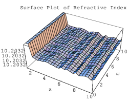
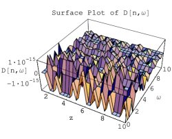
Figure 1: The waves are directed away from the event horizon. The dispersion is found to be normal and anomalous randomly

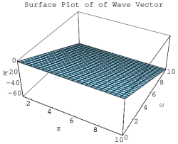
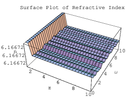
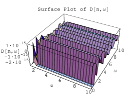
Figure 2: The waves moves towards the event horizon. The dispersion is normal at random points

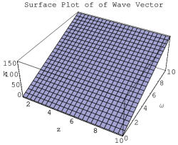
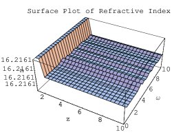
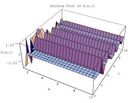
Figure 3: The waves move away from the event horizon. The dispersion is found to be normal and anomalous at random points

Figure 1 shows the graphs of $k$ obtained from Eq.(4.6) whereas Figures 2 and 3 represent values of $k$ obtained from Eq.(4.7). The graph labels A, B and C denote the graphs of the wave vector, the refractive index and change in the refractive index with respect to angular frequency $\omega$ respectively.

Here we are give a brief description of Figure $1$ which helps to access the results for the other figures.

In Figure 1, the wave vector admits positive values which indicates that the waves move away from the event horizon. The refractive index is greater than one throughout the region and increases in a small region $1.2\leq z\leq 1.8,0\leq\omega\leq 10$ with the decrease in $z$. The change in refractive index with respect to angular frequency is positive at random points which shows that the waves disperse normally at those points. The dispersion is anomalous at rest of the points due to negative values of $\frac{dn}{d\omega}$.
The information obtained from Figures 1-3 is given in the following table.

Table I: Direction and refractive index of waves

	Direction of waves	Refractive index ($n$)
		$n>1$ and increases in the region
1	Move away from the event horizon	$1.2\leq z\leq 1.8,0\leq\omega\leq 10$
		with the decrease in $z$
2	Move towards the event horizon	Same as above
3	Same as $1$	Same as above

In Figures $1,2$ and $3$, dispersion is normal as well as anomalous at random points.

5 Rotating Non-Magnetized Hot Plasma

This section is devoted to rotating non-magnetized hot plasma flow. When we consider non-magnetized plasma in rotating background, i.e., $\textbf{B}=0$, the equations of evolution of magnetic field (3.2) and (3.3) are satisfied. We substitute $c_{5}=0,~{}B=0,~{}\lambda=0$ and $c_{6}=0$ in the Fourier analyzed perturbed GRMHD Eqs.(3)-(3) and obtain

$$c_{1}(\frac{-\iota\omega}{\alpha}\rho)+c_{2}(\frac{-\iota\omega}{\alpha}p)+c_{3}(\rho+p)[\frac{-\iota\omega}{\alpha}\gamma^{2}u+(1+\gamma^{2}u^{2})\iota k$$

$$-(1-2\gamma^{2}u^{2})(1+\gamma^{2}u^{2})\frac{u^{\prime}}{u}+2\gamma^{4}u^{2}VV^{\prime}]+c_{4}(\rho+p)\gamma^{2}[(\frac{-\iota\omega}{\alpha}$$

$$+\iota ku)V+u(1+2\gamma^{2}V^{2})V^{\prime}+2\gamma^{2}u^{2}Vu^{\prime}]=0,$$ (5.1)

$$c_{1}[\rho\gamma^{2}u\{(1+\gamma^{2}V^{2})V^{\prime}+\gamma^{2}Vuu^{\prime}\}+\gamma^{2}Vu(\rho^{\prime}+\iota k\rho)]+c_{2}[p\gamma^{2}u$$

$$\times\{(1+\gamma^{2}V^{2})V^{\prime}+\gamma^{2}Vuu^{\prime}\}+\gamma^{2}Vu(p^{\prime}+\iota kp)]+c_{3}[(\rho+p)\gamma^{2}$$

$$\times\{(\frac{-\iota\omega}{\alpha}+\iota ku)\gamma^{2}Vu+(1+2\gamma^{2}u^{2})(1+2\gamma^{2}V^{2})V^{\prime}-\gamma^{2}V^{2}V^{\prime}$$

$$+2\gamma^{2}(1+2\gamma^{2}u^{2})uVu^{\prime}\}+\gamma^{2}V(1+2\gamma^{2}u^{2})(\rho^{\prime}+p^{\prime})]+c_{4}[(\rho+p)$$

$$\{\gamma^{2}(1+\gamma^{2}V^{2})(\frac{-\iota\omega}{\alpha}+\iota ku)+\gamma^{4}u((1+4\gamma^{2}V^{2})uu^{\prime}+4VV^{\prime}(1+$$

$$\gamma^{2}V^{2}))\}+\gamma^{2}u(1+2\gamma^{2}V^{2})(\rho^{\prime}+p^{\prime})]=0,$$ (5.2)

$$c_{1}[\rho\gamma^{2}\{a_{z}+(1+\gamma^{2}u^{2})uu^{\prime}+\gamma^{2}u^{2}VV^{\prime}\}+\gamma^{2}u^{2}(\rho^{\prime}+\iota k\rho)]$$

$$+c_{2}[p\gamma^{2}\{a_{z}+(1+\gamma^{2}u^{2})uu^{\prime}+\gamma^{2}u^{2}VV^{\prime}\}+(p^{\prime}+\iota kp)\times$$

$$(1+\gamma^{2}u^{2})]+c_{3}[(\rho+p)\gamma^{2}\{(1+\gamma^{2}u^{2})(\frac{-\iota\omega}{\alpha}+\iota ku)+u^{\prime}(1+\gamma^{2}u^{2})$$

$$\times(1+4\gamma^{2}u^{2})+2u\gamma^{2}(a_{z}+(1+2\gamma^{2}u^{2})VV^{\prime})\}+2\gamma^{2}u(1+\gamma^{2}u^{2})$$

$$\times(\rho^{\prime}+p^{\prime})]+c_{4}[(\rho+p)\gamma^{4}\{(\frac{-\iota\omega}{\alpha}+\iota ku)uV+u^{2}V^{\prime}(1+4\gamma^{2}V^{2})$$

$$+2V(a_{z}+(1+2\gamma^{2}u^{2})uu^{\prime})\}+2\gamma^{4}u^{2}V(\rho^{\prime}+p^{\prime})]=0,$$ (5.3)

$$c_{1}\rho\gamma^{2}[\frac{-\iota\omega}{\alpha}+u\{a_{z}+\gamma^{2}(VV^{\prime}+uu^{\prime})\}]+c_{2}p[\frac{-\iota\omega}{\alpha}(\gamma^{2}-1)$$

$$+\gamma^{2}u\{a_{z}+\gamma^{2}(VV^{\prime}+uu^{\prime})\}]+c_{3}(\rho+p)\gamma^{2}[\gamma^{2}u(\frac{-2\iota\omega}{\alpha}+\iota ku)$$

$$+(a_{z}+2\gamma^{2}uu^{\prime})(1+2\gamma^{2}u^{2})+\gamma^{2}VV^{\prime}(1+4\gamma^{2}u^{2})]+c_{4}(\rho+p)\gamma^{2}$$

$$\times[\gamma^{2}V(\frac{-2\iota\omega}{\alpha}+\iota ku)+\gamma^{2}uV^{\prime}(1+4\gamma^{2}V^{2})+2\gamma^{2}uV(a_{z}$$

$$+2\gamma^{2}uu^{\prime})]=0.$$ (5.4)

These equations can be used to find dispersion relations.

5.1 Numerical Solutions

For rotating plasma, the velocity assumption can be modified as follows.

• Velocity components: $u=V,~{}x$ and $z$-components of velocity are modified as $u=V=-\sqrt{\frac{1-\alpha^{2}}{2}}$.
  
  Thus, the Lorentz factor becomes

  $$\gamma=1/\sqrt{1-u^{2}-V^{2}}=1/\alpha.$$

This assumption along with the assumptions of time lapse, specific enthalpy, density and pressure given in Section 4, satisfy the GRMHD Eqs.(3.2)-(3) for the region $1.4\leq z\leq 10,0\leq\omega\leq 10$. The determinant of the coefficients of constants in Eq.(LABEL:46)-(5) leads to two dispersion relations. The equation obtained from the real part of the determinant is quartic, i.e.,

$$A_{1}(z)k^{4}+A_{2}(z,\omega)k^{3}+A_{3}(z,\omega)k^{2}+A_{4}(z,\omega)k+A_{5}(z,\omega)=0$$ (5.5)

which yields four values of $k$ out of which two are real and other two are complex conjugate of each other. The imaginary part gives a cubic equation of the form

$$B_{1}(z)k^{3}+B_{2}(z,\omega)k^{2}+B_{3}(z,\omega)k+B_{4}(z,\omega)=0$$ (5.6)

which leads to three roots in which one is real and other two are complex conjugate of each other.

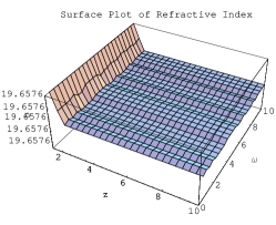
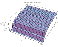
Figure 4: The waves are directed towards the the event horizon. The region shows anomalous dispersion

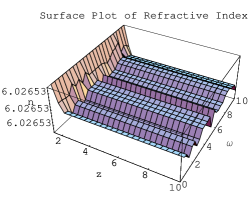
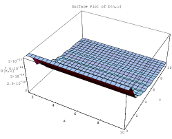
Figure 5: The waves are directed towards the the event horizon. The dispersion is normal

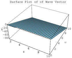
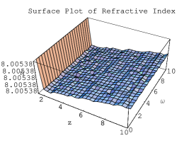
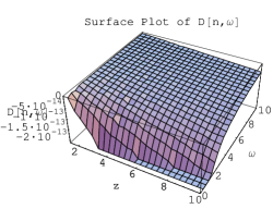
Figure 6: The waves are directed towards the the event horizon. The whole region admits anomalous dispersion

The real values of $k$ obtained from Eq.(5.5) and (5.6) along with respective refractive index and its change with respect to angular frequency are shown in Figures 4, 5 and 6.

The results derived from the Figures 4-6 can be represented in the following tables.

Table II. Direction and refractive index of waves.

	Direction of waves	Refractive index ($n$)
		$n>1$ and increases in the region
4	Move towards the event horizon	$1.4\leq z\leq 1.8,0\leq\omega\leq 10$
		with the decrease in $z$
5	Same as $4$	Same as above
		$n>1$ and increases in the region
6	Same as $4$	$1.4\leq z\leq 1.7,0\leq\omega\leq 10$
		with the decrease in $z$

The regions of normal and anomalous dispersion can be summarized as

Table III. Regions of dispersion.

	Normal dispersion	Anomalous dispersion
4	—	$1.4\leq z\leq 10,0\leq\omega\leq 10$
5	$1.4\leq z\leq 10,0\leq\omega\leq 10$	—
6	—	$1.4\leq z\leq 10,0\leq\omega\leq 10$

6 Rotating Magnetized Hot Plasma

Here, we assume that the plasma is magnetized and rotating. The velocity and magnetic field of fluid are assumed to lie in $xz$ plane. The respective Fourier analyzed perturbed GRMHD equations will remain the same as given by Eqs.(3)-(3) in Section 3.

6.1 Numerical Solutions

We shall use the same values of time lapse, specific enthalpy, density, pressure, $x$ and $z$-components of velocity as given in Sections 4 and 5 with the following restrictions on the magnetic field.

• When we take $u=V$ and $V^{F}=0,$ Eq.(3.8) leads to $\lambda=1$.

• $B=\sqrt{\frac{176}{7}}$.

These restrictions satisfy the GRMHD Eqs.(3.2)-(3) for the region $1.4\leq z\leq 10,0\leq\omega\leq 10$. From Eqs.(3.26) and (3.27), we have $c_{5}=0$. Substituting $c_{5}=0$ in Eqs.(3) and (3)-(3), we obtain a $5\times 5$ matrix of the coefficients of constants. Its determinant leads to two dispersion relations. The real parts give

$$A_{1}(z)k^{4}+A_{2}(z,\omega)k^{3}+A_{3}(z,\omega)k^{2}+A_{4}(z,\omega)k+A_{5}(z,\omega)=0$$ (6.1)

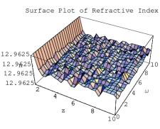
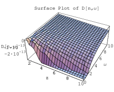
Figure 7: The waves move away from the event horizon. The whole region admits the anomalous dispersion

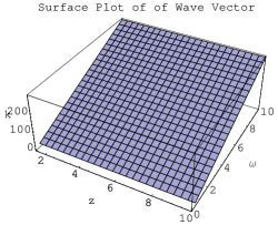
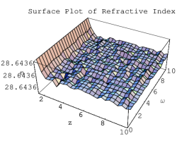
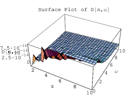
Figure 8: The waves are directed away from the event horizon. The dispersion is normal in most of the region

yielding four values of $k$ out of which two are real and interesting shown in Figures 7 and 8. The imaginary part leads to

$$B_{1}(z)k^{5}+B_{2}(z,\omega)k^{4}+B_{3}(z,\omega)k^{3}+B_{4}(z,\omega)k^{2}+B_{5}(z,\omega)k$$

$$+B_{6}(z,\omega)=0.$$ (6.2)

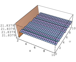
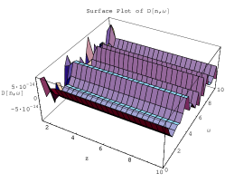
Figure 9: The waves are directed towards the event horizon. Normal dispersion is found at random points

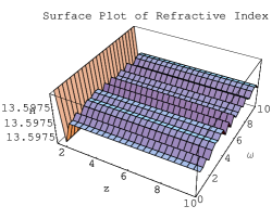
Figure 10: The waves move towards the event horizon. The whole region admits the random points of normal and anomalous dispersion

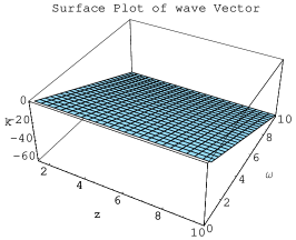
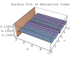
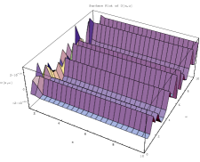
Figure 11: The waves are directed towards the the event horizon. The dispersion is normal at random points

This represents fifth order equation giving five roots in which three are real. These solutions are represented by Figures 9, 10 and 11.

Results related to the direction of waves and the refractive index are given below.

Table IV. Direction and refractive index of waves.

	Direction of waves	Refractive index ($n$)
		$n>1$ and increases in the region
7	Moving away from the event horizon	$1.4\leq z\leq 1.8,0\leq\omega\leq 10$
		with the decrease in $z$
8	Same as $7$	Same as above
		$n>1$ and increases in the region
9	Moving towards the event horizon	$1.4\leq z\leq 1.7,0\leq\omega\leq 10$
		with the decrease in $z$
10	Same as $9$	Same as above
11	Same as $9$	Same as above

The information about the regions of normal and anomalous dispersion obtained from Figures 7-11 is given in the following table.

Table V. Regions of dispersion.

Figure	Normal dispersion	Anomalous dispersion
7	—	$1.4\leq z\leq 10,0\leq\omega\leq 10$
8	$3\leq z\leq 10,1\leq\omega\leq 10$	—
	$2\leq z\leq 10,2\leq\omega\leq 2.4$	$1.8\leq z\leq 10,2.8\leq\omega\leq 3$
	$2\leq z\leq 10,3.41\leq\omega\leq 3.6$	$1.9\leq z\leq 10,3.6\leq\omega\leq 3.8$
	$2\leq z\leq 10,4.2\leq\omega\leq 4.6$	$2.3\leq z\leq 10,4.68\leq\omega\leq 5$
	$2.3\leq z\leq 10,5.4\leq\omega\leq 5.62$	$1.6\leq z\leq 10,5.65\leq\omega\leq 6$
9	$2\leq z\leq 10,6.38\leq\omega\leq 6.6$	$1.8\leq z\leq 10,6.6\leq\omega\leq 6.8$
	$2\leq z\leq 10,7\leq\omega\leq 7.35$	$1.9\leq z\leq 10,7.38\leq\omega\leq 7.6$
	$2\leq z\leq 10,8\leq\omega\leq 8.2$	$2\leq z\leq 10,8.3\leq\omega\leq 8.97$
	$2\leq z\leq 10,9\leq\omega\leq 9.2$	$1.8\leq z\leq 10,9.58\leq\omega\leq 9.84$
	$2\leq z\leq 10,9.9\leq\omega\leq 10$
	$2.1\leq z\leq 10,1.7\leq\omega\leq 2.3$	$2\leq z\leq 10,2.5\leq\omega\leq 2.8$
	$2\leq z\leq 10,4.21\leq\omega\leq 4.6$	$2\leq z\leq 10,4.61\leq\omega\leq 5$
	$2.3\leq z\leq 10,5.1\leq\omega\leq 5.4$	$2\leq z\leq 10,5.41\leq\omega\leq 5.65$
	$2\leq z\leq 10,5.67\leq\omega\leq 6.1$	$1.8\leq z\leq 10,6.14\leq\omega\leq 6.4$
10	$2\leq z\leq 10,7.21\leq\omega\leq 7.6$	$1.8\leq z\leq 10,6.9\leq\omega\leq 7.2$
	$2\leq z\leq 10,8.01\leq\omega\leq 8.2$	$1.7\leq z\leq 10,8.6\leq\omega\leq 8.88$
	$2\leq z\leq 10,8.4\leq\omega\leq 8.6$	$1.8\leq z\leq 10,9.69\leq\omega\leq 9.92$
	$2\leq z\leq 10,9.41\leq\omega\leq 9.65$
	$1.7\leq z\leq 10,1.21\leq\omega\leq 1.4$	$1.7\leq z\leq 10,0.4\leq\omega\leq 0.57$
	$2\leq z\leq 10,2.6\leq\omega\leq 2.77$	$2\leq z\leq 10,3.65\leq\omega\leq 3.85$
	$1.9\leq z\leq 10,3.4\leq\omega\leq 3.6$	$2\leq z\leq 10,5.7\leq\omega\leq 6.1$
	$2\leq z\leq 10,4\leq\omega\leq 4.2$	$2\leq z\leq 10,6.44\leq\omega\leq 6.8$
11	$2\leq z\leq 10,4.61\leq\omega\leq 4.97$	$2\leq z\leq 10,7.3\leq\omega\leq 7.6$
	$2\leq z\leq 10,5.4\leq\omega\leq 5.69$	$2\leq z\leq 10,7.8\leq\omega\leq 8$
	$2\leq z\leq 10,6.9\leq\omega\leq 7.2$	$1.8\leq z\leq 10,8.37\leq\omega\leq 8.6$
	$2\leq z\leq 10,7.6\leq\omega\leq 7.8$	$2.2\leq z\leq 10,9.5\leq\omega\leq 9.81$
	$2\leq z\leq 10,8.01\leq\omega\leq 8.35$
	$2\leq z\leq 10,9.2\leq\omega\leq 9.4$

7 Summary

In this paper, we find the wave properties of hot plasma in Schwarzschild magnetosphere. For this purpose, we have derived the 3+1 GRMHD equations for the scenario. Their component and Fourier analyzed forms are formulated using the specific assumptions. Dispersion relations are calculated for the non-rotating, rotating non-magnetized and rotating magnetized plasmas.

For hot plasma living in non-rotating plasma, our assumptions satisfy the 3+1 GRMHD equations in the region $1.2\leq z\leq 10$. In Figure 1, we have found that the waves are directed away from the event horizon while Figure 2 shows that the waves move towards the event horizon. In Figure 3, the waves are directed away from the event horizon. In all these figures, the dispersion is found to be normal and anomalous randomly.

For the rotating non-magnetized plasma, the assumed parameters satisfy the 3+1 GRMHD equations in the region $1.4\leq z\leq 10$. All the figures indicate that the waves are directed towards the event horizon. In Figure 4, dispersion is anomalous in the whole region while Figure 5 indicates that dispersion is normal throughout the region. In Figure 6, dispersion is anomalous.

For the rotating magnetized plasma, our assumptions satisfy the 3+1 GRMHD equations in the region $1.4\leq z\leq 10$. In Figure 7, the dispersion is anomalous and waves are directed away from the event horizon. Figure 8 shows that the waves move away from the event horizon and dispersion is normal in most of the region. Figures 9, 10 and 11 admit random points of normal dispersion. In these figures, the waves move towards the event horizon.

The summary of results and comparison with previous literature is given as follows.

We compare our results with the previous work on isothermal plasma [23]. We have used here the variable specific enthalpy while in previous work this is constant. Here propagation vector admits both positive and negative values which shows that the waves can move away and towards the event horizon. In the previous work, this always takes negative values which indicates that the waves move towards the event horizon. This comparison shows that variation in specific enthalpy effects the direction of waves. The refractive index is always greater than one in both cases. Dispersion is normal and anomalous at random points as shown by figures in both works. Here the waves move away from the event horizon and disperse normally in most of the region of figure $8$. This shows that there is a chance to obtain information and energy from the magnetosphere. In previous work, waves always move towards the event horizon which means that no information can be extracted from black hole whether dispersion is normal or anomalous. The comparison of the results of cold and hot plasma shows that gas pressure grows the normal dispersion.

Table VI. Comparison of results.

Results	Previous work	Recent work
Direction of waves	Towards the event horizon	Away from the event
		horizon
Dispersion	Normal at random points	Normal in most of the
		region in Figure 8
Conclusion	No information can be	A chance to obtain
	extracted	information from
		magnetosphere

It is concluded that the hot plasma waves in the Schwarzschild magnetosphere can have an escape towards the outer end of the magnetosphere.

Acknowledgment: We would like to thank Dr. Umber Skeikh for the fruitful discussions during this work.

Appendix A

This appendix contains the GRMHD equations for the general line element and the Schwarzschild planar analogue. The set of Maxwell equations and conservation laws under the influence of gravitational field are collectively known as GRMHD equations. The hot plasma model includes the mass, momentum and energy conservation laws. The GRMHD equations for the general line element, given by Eq.(2.1), are [23]

$$\frac{d\textbf{B}}{d\tau}+\frac{1}{\alpha}(\textbf{B}.\nabla)\beta+\theta\textbf{B}=\frac{1}{\alpha}\nabla\times(\alpha\textbf{V}\times\textbf{B}),$$ (A1)

$$\nabla.\textbf{B}=0,$$ (A2)

$$\frac{D\rho_{0}}{D\tau}+\rho_{0}\gamma^{2}\textbf{V}.\frac{D\textbf{V}}{D\tau}+\frac{\rho_{0}}{\alpha}\left\{\frac{g,_{t}}{2g}+\nabla.(\alpha\textbf{V}-\beta)\right\}=0,$$ (A3)

$$\left\{\left(\rho_{0}\mu\gamma^{2}+\frac{\textbf{B}^{2}}{4\pi}\right)\gamma_{ij}+\rho_{0}\mu\gamma^{4}V_{i}V_{j}-\frac{1}{4\pi}B_{i}B_{j}\right\}\frac{DV^{j}}{D\tau}$$

$$+\rho_{0}\gamma^{2}V_{i}\frac{D\mu}{D\tau}-\left(\frac{\textbf{B}^{2}}{4\pi}\gamma_{ij}-\frac{1}{4\pi}B_{i}B_{j}\right)V^{j}_{|k}V^{k}=-\rho_{0}\gamma^{2}\mu\{a_{i}$$

$$-\frac{1}{\alpha}\beta_{j|i}V^{j}-(\pounds_{t}\gamma_{ij})V^{j}\}-p_{|i}+\frac{1}{4\pi}(\textbf{V}\times\textbf{B})_{i}\nabla.(\textbf{V}\times\textbf{B})$$

$$-\frac{1}{8\pi\alpha^{2}}(\alpha\textbf{B})^{2}_{|i}+\frac{1}{4\pi\alpha}(\alpha B_{i})_{|j}B^{j}-\frac{1}{4\pi\alpha}(\textbf{B}\times\{\textbf{V}\times[\nabla\times$$

$$(\alpha\textbf{V}\times\textbf{B})-(\textbf{B}.\nabla)\beta]+(\textbf{V}\times\textbf{B}).\nabla\beta\})_{i},$$ (A4)

$$\frac{d}{d\tau}(\gamma^{2}\mu\rho_{0})-\frac{dp}{d\tau}+\theta((\gamma^{2}\rho_{0}\mu-p)+\frac{1}{8\pi}((\textbf{V}\times\textbf{B})^{2}+\textbf{B}^{2}))$$

$$+\frac{1}{2\alpha}\{\gamma^{2}\rho_{0}\mu V^{i}V^{j}+p\gamma^{ij}-\frac{1}{4\pi}((\textbf{V}\times\textbf{B})^{i}(\textbf{V}\times\textbf{B})^{j}$$

$$+B^{i}B^{j})+\frac{1}{8\pi}((\textbf{V}\times\textbf{B})^{2}+\textbf{B}^{2})\gamma^{ij}\}\pounds_{t}\gamma_{ij}+\mu\rho_{0}\gamma^{2}\textbf{V}.\textbf{a}$$

$$+\mu\rho_{0}\gamma^{4}\textbf{V}.(\textbf{V}.\nabla)\textbf{V}-\frac{1}{2\pi}\textbf{a}.((\textbf{V}\times\textbf{B})\times\textbf{B})-\frac{1}{4\pi}(\nabla\times$$

$$(\textbf{V}\times\textbf{B})).\textbf{B}-\frac{1}{\alpha}\left\{\mu\rho_{0}\gamma^{2}\textbf{V}.(\textbf{V}.\nabla)\beta+p(\nabla.\beta)-\frac{1}{4\pi}\textbf{B}.(\textbf{B}.\nabla)\beta\right.$$

$$-\frac{1}{4\pi}(\textbf{V}\times\textbf{B}).\{(\textbf{V}\times\textbf{B}).\nabla\}\beta\left.+\frac{1}{8\pi}((\textbf{V}\times\textbf{B})^{2}+\textbf{B}^{2})(\nabla.\beta)\right\}$$

$$+\frac{1}{4\pi}\left[(\textbf{V}\times\textbf{B}).(\textbf{a}\times\textbf{B})+2(\textbf{V}\times\textbf{B}).\frac{d}{d\tau}(\textbf{V}\times\textbf{B})\right.$$

$$-\frac{1}{\alpha}(\textbf{V}\times\textbf{B}).\{(\textbf{V}\times\textbf{B}).\nabla\}\beta+\theta(\textbf{V}\times\textbf{B}).(\textbf{V}\times\textbf{B})$$

$$\left.+\textbf{B}.\frac{d\textbf{B}}{d\tau}\right]=0.$$ (A5)

For the Schwarzschild planar analogue, $\beta$, $\theta$ and $\pounds_{t}\gamma_{ij}$ vanish, the perfect GRMHD equations take the following form

$$\frac{\partial\textbf{B}}{\partial t}=\nabla\times(\alpha\textbf{V}\times\textbf{B}),$$ (A6)

$$\nabla.\textbf{B}=0,$$ (A7)

$$\frac{\partial\rho_{0}}{\partial t}+(\alpha\textbf{V}.\nabla)\rho_{0}+\rho_{0}\gamma^{2}\textbf{V}.\frac{\partial\textbf{V}}{\partial t}+\rho_{0}\gamma^{2}\textbf{V}.(\alpha\textbf{V}.\nabla)\textbf{V}$$

$$+\rho_{0}{\nabla.(\alpha\textbf{V})}=0,$$ (A8)

$$\{(\rho_{0}\mu\gamma^{2}+\frac{\textbf{B}^{2}}{4\pi})\delta_{ij}+\rho_{0}\mu\gamma^{4}V_{i}V_{j}-\frac{1}{4\pi}B_{i}B_{j}\}(\frac{1}{\alpha}\frac{\partial}{\partial t}+\textbf{V}.\nabla)V^{j}$$

$$-(\frac{\textbf{B}^{2}}{4\pi}\delta_{ij}-\frac{1}{4\pi}B_{i}B_{j})V^{j},_{k}V^{k}+\rho_{0}\gamma^{2}V_{i}\{\frac{1}{\alpha}\frac{\partial\mu}{\partial t}+(\textbf{V}.\nabla)\mu\}$$

$$=-\rho_{0}\mu\gamma^{2}a_{i}-p,_{i}+\frac{1}{4\pi}(\textbf{V}\times\textbf{B})_{i}\nabla.(\textbf{V}\times\textbf{B})-\frac{1}{8\pi\alpha^{2}}(\alpha\textbf{B})^{2},_{i}$$

$$+\frac{1}{4\pi\alpha}(\alpha B_{i}),_{j}B^{j}-\frac{1}{4\pi\alpha}[\textbf{B}\times\{\textbf{V}\times(\nabla\times(\alpha\textbf{V}\times\textbf{B}))\}]_{i},$$ (A9)

$$\gamma^{2}\frac{1}{\alpha}\frac{\partial}{\partial t}(\mu\rho_{0})-\frac{1}{\alpha}\frac{\partial p}{\partial t}+\rho_{0}\mu\gamma^{2}(\textbf{V}.\textbf{a})+\rho_{0}\mu\gamma^{4}\textbf{V}.(\textbf{V}.\nabla)\textbf{V}$$

$$-\frac{1}{2\pi}\textbf{a}.\{(\textbf{V}\times\textbf{B})\times\textbf{B}\}-\frac{1}{4\pi}(\nabla\times(\textbf{V}\times\textbf{B})).\textbf{B}$$

$$+\frac{1}{4\pi}\left\{2\frac{1}{\alpha}(\textbf{V}\times\textbf{B}).\frac{\partial}{\partial t}(\textbf{V}\times\textbf{B})+(\textbf{V}\times\textbf{B}).(\textbf{a}\times\textbf{B})\right.$$

$$\left.+\textbf{B}.\frac{1}{\alpha}\frac{\partial\textbf{B}}{\partial t}\right\}=0.$$ (A10)

	A	B	C

	A	B	C

	A	B	C

	A	B	C

	A	B	C

	A	B	C

	A	B	C

	A	B	C

	A	B	C

References

• [1] T. Regge and J. A. Wheeler: Phy. Rev. 108(1957)1063.
• [2] F. J. Zerilli: Phys. Rev. D2(1970)2141; J. Math. Phys. 11(1970)2203; Phys. Rev. Lett. 24(1970)737.
• [3] R. H. Price: Phys. Rev. D5(1972)2419; Phys. Rev. D5(1972)2439.
• [4] P. P. Fiziev: J. Phys. Conf. Ser. 66(2007)012016.
• [5] R. S. Hanni and R. Ruffini: Phys. Rev. D8(1973)3259.
• [6] J. Sakai and T. Kawata: J. Phys. Soc. Jpn. 49(1980)747.
• [7] R. Arnowitt, S. Deser and C. W. Misner: Gravitation: An Introduction to Current Research (John Wiley & Sons, New York, 1962).
• [8] J. A. Wheeler: Battelle Rencontres: 1967 Lectures in Mathematics and Physics eds. C. DeWitt and J. A. Wheeler ( W.A. Benjamin, Inc., New York, 1968)
• [9] D. A. Macdonald and W. -M. Suen: Phys. Rev. D32(1985)848.
• [10] K. S. Thorne and J. B. Hartle: Phys. Rev. D31(1985)1815.
• [11] K. S. Thorne and D. A. Macdonald: Mon. Not. R. Astron. Soc. 198(1982)339; Mon. Not. R. Astron. Soc. 198(1982)345.
• [12] Black Hole: The Membrane Paradigm eds. K. S. Thorne, R. H. Price and D. A. Macdonald (Yale University Press, New Haven, 1986).
• [13] K. A. Holcomb and T. Tajima: Phys. Rev. D40(1989)3809.
• [14] K. A. Holcomb: Astrophys. J. 362(1990)381.
• [15] C. P. Dettmann, N. E. Frankel and V. Kowalenke: Phys. Rev. D48(1993)5655.
• [16] V. Buzzi, K. C. Hines and R. A. Treumann: Phys. Rev. D51(1995)6663; Phys. Rev. D51(1995)6677.
• [17] M. H. Ali and H. Atiqur Rahman, Transverse Wave Propagation in Relativistic Two-fluid Plasmas around Schwarzschild-de Sitter Black Hole, Int. J. Theo. Phys. (accepted).
• [18] X. -H. Zhang: Phys. Rev. D39(1989)2933.
• [19] X. -H. Zhang: Phys. Rev. D40(1989)3858.
• [20] M. Sharif and U. Sheikh: Gen. Relat. Gravit. 39(2007)1437.
• [21] M. Sharif and U. Sheikh: Gen. Relat. Gravit. 39(2007)2095; Int. J. Mod. Phys. A23(2008)1417; J. Korean Phys. Soc. 52(2008)152.
• [22] M. Sharif and U. Sheikh: J. Korean Phys. Soc. 53(2008)2198.
• [23] U. Sheikh: Ph.D. Thesis, University of the Punjab Lahore (2008).
• [24] M. Sharif and G. Mustafa: Canadian J. Phys. 86(2008)1265.
• [25] S. Shepared: Sonet/SDH Demystified (McGraw-Hill Companies, Inc, U.S.A, 2001) p.103.
• [26] A. C. Das: Space Plasma Physics: An Introduction (Narosa Publishing House, New Dehli, 2004) p.75.
A B C
Refer to caption Refer to caption Refer to caption