Pulsar magnetic alignment and the pulsewidth-age relation

Abstract

Using pulsewidth data for 872 isolated radio pulsars we test the hypothesis that pulsars evolve through a progressive narrowing of the emission cone combined with progressive alignment of the spin and magnetic axes. The new data provide strong evidence for the alignment over a time-scale of about $1\,$Myr with a log standard deviation of around 0.8 across the observed population. This time-scale is shorter than the time-scale of about $10\,$Myr found by previous authors, but the log standard deviation is larger. The results are inconsistent with models based on magnetic field decay alone or monotonic counter-alignment to orthogonal rotation. The best fits are obtained for a braking index parameter, $n_{\gamma}\approx 2.3$, consistent the mean of the six measured values, but based on a much larger sample of young pulsars. The least-squares fitted models are used to predict the mean inclination angle between the spin and magnetic axes as a function of log characteristic age. Comparing these predictions to existing estimates it is found that the model in which pulsars are born with a random angle of inclination gives the best fit to the data. Plots of the mean beaming fraction as a function of characteristic age are presented using the best-fitting model parameters.

1 INTRODUCTION

One of the greatest of the many mysteries of radio pulsars is their evolutionary histories. As pulsars age, powerful electromagnetic torques act to increase the rotation period, $P$, of the strongly magnetized neutron star, causing the spin-frequency, $\nu=1/P$, to decrease over time, a phenomenon known as spin-down. This can be described by the equation

$$\dot{\nu}=-K\nu^{n}\mbox{~{},}$$ (1)

where $n$ is a parameter known as the braking index, with $n=3$ for a magnetic dipole rotating in a vacuum. The spin-down torque acting on the star is proportional to $\dot{\nu}$, and it decays over time as $\dot{\nu}$ decreases.

There is also evidence that $K$ is not constant, but rather is also changing over time. The surface dipole magnetic field strength at the magnetic equator, assuming that the spin and magnetic axes are orthogonal, is conventionally given by $B_{\mathrm{surf}}=3.2\times 10^{19}(P\dot{P})^{1/2}\,\mbox{G}$; at the magnetic poles the field strength is $2B_{\mathrm{surf}}$ (Lyne & Smith, 2006). $B_{\mathrm{surf}}$ tends to be bigger for younger pulsars than for older ones having a large spin-down age, $t_{s}{}\equiv{}P/\left[(n-1)\dot{P}\right]$. This in turn suggests that $K$ tends to reduce with increasing age, and much conjecture remains about the origin(s) of this evolution.

Many authors have argued that the main contributor to the $K$-evolution is the progressive alignment of the spin and magnetic axes: e.g. Candy & Blair (1983), Candy & Blair (1986), Lyne & Manchester (1988), Xu & Wu (1991), Kuz’min & Wu (1992), Candy (1993), Pandey & Prasad (1996), Tauris & Manchester (1998) and Weltevrede & Johnston (2008). But McKinnon (1993) and Gil & Han (1996) have argued in favour of a random distribution of the inclination angles between the angular velocity and magnetic axes and against magnetic alignment. Others have favoured magnetic field decay (e.g. Narayan & Ostriker, 1990), while there are also authors who argue for continuing counter-alignment to eventual orthogonality of the axes, via an electromagnetic torque exerted by magnetospheric electric currents flowing on open field lines (Beskin et al., 1984).

According to Jones (1976), pulsars initially counter-align (via a strongly temperature-dependent dissipative torque in the fluid interior) to reach the orthogonal rotator state after about $10^{3}\,$yr, where they remain for $10^{4}$–$10^{5}\,$yr (while the dissipative torque decays as the interior cools), after which alignment (via electromagnetic torque) occurs.

If $K$ were constant, the braking index $n$ would be equal to the apparent braking index,

$$n_{\mathrm{app}}\equiv{\nu\ddot{\nu}}/{\dot{\nu}^{2}}=2-{P\ddot{P}}/{\dot{P}^{2}}\mbox{~{}.}$$ (2)

If $\ddot{\nu}$ can be determined from observations of a pulsar, then $n_{\mathrm{app}}$ can be computed. However, if $K$ is varying, then in general $n_{\mathrm{app}}\neq{}n$. Some authors (eg. Johnston & Galloway, 1999; Tauris & Konar, 2001) have argued that, for pulsars of moderate age, $n_{\mathrm{app}}$ exceeds the value of 3 that corresponds to magnetic dipole radiation. This could be taken to imply that either magnetic alignment or field decay must be occurring. However, it is likely that recovery from unseen pulsar glitches is the principal contribution to measured variations in $\dot{P}$ (Wang et al., 2001) for these pulsars.

In this paper, we shall use the pulsar evolution models from Candy & Blair (1983, hereafter CB83), Candy & Blair (1986, hereafter CB86) and Candy (1993, hereafter C93), which all invoke a progressive alignment of the spin and magnetic axes. The CB83 model develops the pulsewidth-age relation on the assumption that all pulsars move along the same evolutionary track, differing only in age and orientation with respect to Earth. The CB86 model relaxes this assumption and allows a distribution of alignment time-scales, as well as a time-varying relationship between characteristic and actual age. The C93 models additionally allow a distribution of initial inclination angles. All of these models predicted a minimum in the mean pulsewidth as a function of characteristic age and provided a good fit to the available data, consisting of 293 pulsewidth values from the Manchester & Taylor (1981) catalogue.

Here we use the ATNF (Australia Telescope National Facility) pulsar catalogue (Manchester et al., 2005), version 1.35, to investigate pulsar evolution through magnetic alignment using the Candy–Blair models. This contemporary catalogue contains much larger data sets of 872 and 1420 isolated radio pulsars with 10 per cent and 50 per cent intensity pulsewidth values, $W_{10}$ and $W_{50}$. It also contains many more old pulsars than was previously the case, which tend to have lower radio luminosities. It thus allows a more precise analysis of pulsar evolution. As a consistency check, we also examine separately those pulsars with pulsewidths measured during the Parkes multibeam pulsar survey (Manchester et al., 2001; Lorimer et al., 2006), giving $W_{10}$ and $W_{50}$ data sets of 377 and 934 pulsars respectively.

The paper is structured as follows. Section 2 presents a summary of the theory of alignment between the spin and magnetic axes; Section 3 gives a mathematical description of pulsewidth evolution; in Section 4 we least-squares fit the evolutionary pulsewidth models to the $W_{10}$ and $W_{50}$ data as functions of characteristic age; in Section 5 we further analyse these results, in particular comparing them to the inclination angle estimates of Rankin (1993b) and Gould (1994); and conclusions are presented in Section 6.

2 Magnetic alignment theory

2.1 Evolution in true age

The Candy–Blair pulsar evolution models are based on two effects. One is progressive alignment of the spin and magnetic axes, for which the formula describing the alignment phase of the Jones (1976) model is adopted: this has an exponential decay of the sine of the magnetic-spin inclination angle, $\alpha$, from its initial value $\alpha_{0}$:

$$\sin\alpha(t)=\exp(-t/\tau)\,\sin\alpha_{0}\,,$$ (3)

where $t$ is the pulsar’s age and $\tau$ is the alignment time-scale. The alignment has a simple electromechanical origin: the electromagnetic radiation emitted by an oblique rotating dipole results in a torque on the star that causes the angular velocity axis to migrate through the neutron star toward alignment with the magnetic axis.

The second effect is progressive narrowing of the emission cone, described by a power-law dependence of its half-angle, $\rho$, on the rotation period, $P$:

$$\rho(t)\propto P^{-\gamma}(t)\,,$$ (4)

with $\gamma$ a positive constant having a value between $1/3$ and $2/3$ (Gunn & Ostriker, 1970; Ruderman & Sutherland, 1975; Lyne & Manchester, 1988; Rankin, 1993a).

For a pulsar with constant rotational inertia and fixed magnetic moment vector, the rotation period evolves according to $\dot{P}P^{n-2}$ = constant. It was pointed out long ago (Phinney & Blandford, 1981) that this simple rule is incompatible with the observed distribution of pulsars in the $P$–$\dot{P}$ plane, conflicting with stationary ‘flow’ through that plane to pulsar ‘death’ at advanced ages. However, alignment produces an effective reduction in the magnetic moment, reducing the torque in proportion to $\sin{{}^{2}}\alpha$; so, in the Jones model, the period evolves according to (Phinney & Blandford, 1981)

$$\dot{P}P^{n-2}\propto\exp(-2t/\tau)\,,$$ (5)

with $n$ (the braking index) constant.

Equation (5) integrates to give:

$$P^{n-1}(t)=P{{}_{\infty}}^{n-1}+(P{{}_{0}}^{n-1}-P{{}_{\infty}}^{n-1})\exp(-2t/\tau)\,,$$ (6)

where $P_{0}$ is the pulsar’s initial period and $P_{\infty}$ is its limiting period as $t\rightarrow\infty$. Assuming that pulsars eventually slow substantially from their initial spin period, $P_{0}\ll P_{\infty}$, we can approximate equation (6) by

$$P(t)\approx P_{\infty}[\,1-\exp(-2t/\tau)\,]^{1/(n-1)}\,.$$ (7)

Using (7) for $P(t)$ in (4) for $\rho(t)$ yields a simple approximation for the evolution of $\rho$, expressed directly in terms of $t$:

$$\rho(t)\approx\rho_{\infty}[\,1-\exp(-2t/\tau)\,]^{-\gamma/(n-1)}\,,$$ (8)

where $\rho_{\infty}$ is the limiting emission cone half-angle as $t\rightarrow\infty$.

We note that, because $P_{0}$ has effectively been taken as zero in going from (6) to (7) for $P(t)$, equation (8) is not applicable to the very youngest pulsars: for $t\ll\tau/2$ it reduces to

$$\rho(t)/\rho_{\infty}\approx(\tau/2t)^{\gamma/(n-1)}\,,$$ (9)

which diverges as $t\rightarrow 0$. For the typical parameter values (see Section 4.3 Table 3) $\gamma=1/2,$ $n=2.3,$ $\tau=1\times 10^{6}\,$yr, and $\rho_{\infty}=2-5\degr$, equation (9) gives $\rho(t)\approx 11\rho_{\infty}\approx 22-55\degr$ for $t\approx 1000\,$yr. As only one known pulsar is this young, the divergence is outside the age range we can analyse, and the approximation (8) for $\rho(t)$ is valid for our purposes.

2.2 Evolution in characteristic age

A pulsar’s spin-down age, $t_{s}{}\equiv{}P/\left[(n-1)\dot{P}\right]$, depends on $n$, which is going to be a variable in our fitting procedure below. Instead of the spin-down age, from here on we use the the characteristic age which is defined to be

$$t_{c}\equiv{P}/\left({2\dot{P}}\right)\mbox{~{}.}$$ (10)

The characteristic age is independent of $n$ and corresponds to the spin-down age in the case $n=3$. Its use enables us to show fittings for different $n$ on one plot using the same characteristic-age data. Inserting equation (7) for $P(t)$, we find that $t_{c}$ is related to the pulsar’s actual age, $t$, by:

$$t_{c}(t)/\tau = [\,(n-1)/4\,][\,\exp(2t/\tau)-1\,]$$ (11)

$$\mbox{or~{}~{}}\exp[2t(t_{c})/\tau] = 1+(4t_{c})/[(n-1)\tau]\mbox{~{}.}$$ (12)

Note that factors of $2/(n-1)$ effectively rescale $t_{c}$ to $t_{s}{}$ in these equations.

It follows from equation (11) that $t_{c}\approx(n-1)t/2$ for relatively young pulsars (young compared with the spin-down time-scale); for old pulsars, $t_{c}/\tau$ increases as an exponential function of $t/\tau$. The characteristic and actual ages coincide for relatively young pulsars in the dipole rotator case, for which $n=3$.

The $t_{c}$–$t$ relation enables equations (3), (7) and (8) for $\alpha$, $P$ and $\rho$ to be re-expressed in terms of $t_{c}$ – which has the advantage of being directly determined from the measured quantities $P$ and $\dot{P}$ – instead of in terms of $t$:

$$\sin\alpha(t_{c})\! = \!\left(\sin\alpha_{0}\right)\left[1+{4t_{c}}/{(n-1)\tau}\right]^{-1/2}\mbox{~{},}$$ (13)

$$P(t_{c})\! = \!P_{\infty}\left[1+{(n-1)\tau}/{4t_{c}}\right]^{-1/(n-1)}\mbox{~{},}$$ (14)

$$\mbox{and}\hskip 14.22636pt\rho(t_{c})\! = \!\rho_{\infty}\left[1+{(n-1)\tau}/{4t_{c}}\right]^{\gamma/(n-1)}\mbox{~{}.}$$ (15)

Equation (15) describes an emission-cone half-width that decreases quite rapidly with time for young pulsars; consequently, the observed pulsewidths should decrease with age for the youngest pulsars. The alignment of the spin and magnetic axes, described by equation (13), should cause an increase in the observed pulsewidths for older pulsars, as the pulse will occupy a larger fraction of a complete rotation. The combination of these two processes should lead to a minimum in the observed angular pulsewidths for pulsars of moderate ages (CB83).

Note that taking the derivative of equation (6) and using equation (10) for $t_{c}$ gives (cf. equation (2))

$$n_{\mathrm{app}}=n+4{t_{c}}/{\tau}\mbox{~{},}$$ (16)

showing that the apparent braking index increases with characteristic age.

2.3 The parameters of the theory

Equations (13), (14) and (15) – expressing the evolution of the magnetic-spin inclination angle, the pulsar period and the emission cone half-angle in terms of a pulsar’s characteristic age – can conveniently be re-written in terms of a normalized dimensionless characteristic age:

$$T_{c}\equiv 2t_{c}/[(n-1)\tau]\;,$$ (17)

which reduces to $t_{c}/\tau$ in the dipole rotator $(n=3)$ case. Thus:

$$\sin\alpha(T_{c})\! = \!\left(\sin\alpha_{0}\right)(1+2T_{c})^{-1/2}\mbox{~{},}$$ (18)

$$P(T_{c})\! = \!P_{\infty}[1+(2T_{c})^{-1}]^{-1/(n-1)}\mbox{~{},}$$ (19)

$$\mbox{and~{}~{}}\rho(T_{c})\! = \!\rho_{\infty}[1+(2T_{c})^{-1}]^{\gamma/(n-1)}\mbox{~{}.}$$ (20)

In the equations used for the pulsewidth modelling below, namely (13) and (15), or (18) and (20), for $\alpha(t_{c})$ and $\rho(t_{c})$, $n$ appears only in the two combinations $\gamma/(n-1)$ and $(n-1)\tau$. Hence there are only four basic independent parameters in the Candy-Blair alignment models. Later we will set $\gamma=1/2$, consistent with the $\gamma$ values found by other authors (e.g. Rankin, 1993a; McKinnon, 1993; Gould, 1994). Hence, it is convenient in this study to define the four independent parameters to be $\alpha_{0}$, $\rho_{\infty}$, $n_{\gamma}$ and $\tau_{\gamma}$, where

$$n_{\gamma} \equiv 1+\left(n-1\right)/(2\gamma)\mbox{~{},~{}and}$$ (21)

$$\tau_{\gamma} \equiv 2\gamma\,\tau\mbox{~{},}$$ (22)

since these last two parameters are normalized to the $\gamma=1/2$ case. In terms of these parameters, the two combinations $\gamma/(n-1)$ and $(n-1)\tau$ become

$$\gamma/(n-1) = 1/\left[2\left(n_{\gamma}-1\right)\right]\mbox{~{},~{}and}$$ (23)

$$(n-1)\,\tau = (n_{\gamma}-1)\tau_{\gamma}\mbox{~{},}$$ (24)

and equation (16) gives

$$n_{\mathrm{app}}-1=2\gamma\left(n_{\gamma}-1+\frac{t_{c}}{\tau_{\gamma}}\right)\mbox{~{}.}$$ (25)

3 PULSEWIDTH EVOLUTION DESCRIPTION

3.1 Mean pulsewidths

For an individual pulsar, the observed angular pulsewidth is given as a function of $\alpha,\rho$ and $\zeta$ by

$$W(\alpha,\rho,\zeta)=2\arccos{\Big{(}\frac{\cos\rho-\cos\alpha\cos\zeta}{\sin\alpha\sin\zeta}\Big{)}}\,,$$ (26)

where $\zeta$ is the angle between the observer’s direction and the pulsar’s spin axis (Manchester & Taylor, 1977, p. 218). The strong dependence on the orientation of the observer with respect to the spin axis leads to a wide scatter in the pulsewidth values, so we need to take a mean pulsewidth for pulsars with certain values of $\alpha$ and $\rho$.

The mean pulsewidth is obtained by integrating (26) over the angular extent of the emission beam:

$$\left<{W}\right>\!(\alpha,\rho)=\int_{\mid\alpha-\rho\mid}^{\alpha+\rho}W(\alpha,\rho,\zeta)P(\zeta)\mathrm{d}\zeta\mbox{~{},}$$ (27)

in which $P(\zeta)\mathrm{d}\zeta$ is the probability that the angle between the spin axis and the observer’s direction is in the range $\zeta$ to $\zeta+\mathrm{d}\zeta$. The integration is over all angles $\zeta$ for which emission is both directed toward the observer and seen as pulsed.

The limits of integration in (27) for $\left<{W}\right>\!(\alpha,\rho)$ are explained by means of Fig. 1. For a pulsar that is not too close to alignment, such that the emission beam does not contain the rotation axis (Fig. 1, left), $\alpha>\rho$ and the beam is intercepted for a part (but not all) of the rotation period if $\zeta$ is in the range $\alpha-\rho$ to $\alpha+\rho$. For a pulsar that is close to alignment, with the emission beam containing the rotation axis (Fig. 1, right), $\alpha<\rho$ and the range $\zeta<\rho-\alpha$ is excluded, as some part of the beam is then always directed toward the observer, assuming the emission cone to be filled.

We take $\alpha\leq 90\degr$; the choice of first or second quadrant for $\alpha$ is a matter of convention, switching it between hemispheres being equivalent to reversing the sense of the neutron star’s rotation. The beam, however, can extend into the other hemisphere, which it will do if $\alpha+\rho>\pi/2$, as expected for young pulsars with wide beams. If a pulsar produces observable radio emission from both poles, then this will be observed as a main pulse and interpulse, provided that the pulsar is nearly orthogonal or the pulsar beams are wide. However, the mean pulsewidths referred to here are for emission from only one of these poles, not the combined main pulse – interpulse width.

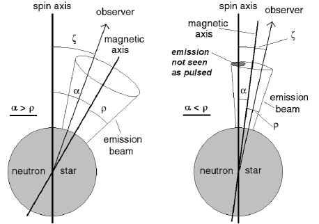
Figure 1: Pulsar emission relative to a distant observer, assuming a circular cone of emitted radiation, with the magnetic-spin inclination angle $\alpha$ either greater (left) or less (right) than the emission cone half-angle $\rho$. In the latter case, the emission cone encloses the spin axis, and there may be little or no modulation; in particular, to observers in the cone $\zeta<\rho-\alpha$, the emission cone is continuously visible. The left-hand diagram depicts the usual case of a pulsar with moderate values of $\alpha$ and $\rho$, typical of mature-aged pulsars. The right-hand diagram depicts a pulsar with a thin beam and nearly aligned spin and magnetic axes, typical of old pulsars in the Candy-Blair theory and the Jones model.

On taking pulsar spin axes to be randomly directed with respect to observers, and normalizing over the angular extent of the emission cone, the probability distribution for $\zeta$ becomes:

$$P(\zeta)\mathrm{d}\zeta=(\sin{\zeta}\mathrm{d}\zeta/2)/f_{b}(\alpha,\rho)\mbox{~{},}$$ (28)

where $f_{b}$ is the ‘beaming fraction’, which measures the fraction of the sky swept out by the beam. Equation (28) is the ratio of the surface area of a ring on a sphere, corresponding to observers in the range $\zeta$ to $\zeta+\mathrm{d}\zeta$, to the surface area of the sphere swept out by the beam.

The surface area of the part of a sphere between co-latitudes $\theta_{1}$ and $\theta_{2}$, normalized to the surface area of a sphere, is

$$\sin\left[(\theta_{1}+\theta_{2})/2\right]\sin\left[(\theta_{2}-\theta_{1})/2\right]\mbox{~{}.}$$ (29)

Inserting $\theta_{1}=\left|\alpha-\rho\right|$ and $\theta_{2}=\alpha+\rho$ gives the beaming fraction:

$$f_{b}(\alpha,\rho)=\sin{\alpha}\sin{{\rho}}\,,$$ (30)

applicable to both situations depicted in Fig. 1.

We note that Tauris & Manchester (1998, eq. (7)) use a different beaming fraction for the case $\alpha<\rho$, namely $1-\cos(\alpha+\rho)$, which results from integration over 0 to $\alpha+\rho$. As they remark, there may be little or no modulation when $\alpha<\rho$, and we prefer to exclude the ‘continuously seen’ cone, $\zeta<\rho-\alpha$ (Fig. 1, right).

3.2 Evolution modelling

The evolutionary time dependence of $\alpha$ and $\rho$, equations (3) and (8), results in a mean pulsewidth, $\left<W\right>\!(\alpha,\rho)$, that is a function of time only, $\left<W\right>\!(t)$. This function is to be treated as a density, $\left<W\right>\!(t)\,\mathrm{d}t$ giving the mean pulsewidth of pulsars aged between $t$ and $t+\mathrm{d}t$. The age of the pulsars will here be measured in terms of their log characteristic age, $\log{t_{c}}$, and will be binned with respect to that variable. Under the change of variables $t\rightarrow t(\log t_{c})$, we have

$$\left<{W}\right>\!(t)\mathrm{d}t = \left<{W}\right>\!\left(t(\log{t_{c}})\right)\,\frac{\mathrm{d}t}{\mathrm{d}\left(\log{t_{c}}\right)}\mathrm{d}\left(\log{t_{c}}\right)$$ (31)

$$\equiv \left<{W}\right>\!(\log{t_{c}})f_{t}\mathrm{d}\left(\log{t_{c}}\right)\mbox{~{}.}$$ (32)

The factor $f_{t}\left(t_{c}\right)$ is given by

$$f_{t}\equiv\frac{\mathrm{d}t}{\mathrm{d}\log{t_{c}}}=\frac{\tau\ln{10}}{2}\left(1+\frac{(n-1)\tau}{4t_{c}}\right)^{-1}\,,$$ (33)

where the $t$–$t_{c}$ relation, equation (12), has been used. So $f_{t}\left(t_{c}\right)$ increases monotonically from $(\ln{10})2t_{c}/(n-1)$ for young pulsars, flattening to $(\ln{10})\tau/2$ for old ones.

To allow for variations between the evolutionary histories of different pulsars, CB86 and C93 relaxed the assumptions that all pulsars are born with the same inclination angle and have the same alignment time-scale, $\alpha_{0}$ and $\tau$ respectively. Instead, these are replaced by a probability distribution function, $P(\alpha_{0})$, for initial inclination angles (see Section 3.3), and a log-normal distribution of alignment time-scales:

$$P(\log{\tau})=\frac{1}{\sqrt{2\pi}\sigma_{\log}}\exp\left[-\frac{1}{2}\left(\frac{\log{\tau}-\mu_{\log}}{\sigma_{\log}}\right)^{2}\right]\mbox{,}$$ (34)

where $\mu_{\log}$ and $\sigma_{\log}$ are the mean and standard deviation of the logarithm of the time-scale distribution, $\log{\tau}$. If the normalized parameters $n_{\gamma}$ and $\tau_{\gamma}$ that were introduced in equations (21)–(24) are used, then $\tau_{\gamma}$ has a log-normal distribution with mean

$$\mu_{\gamma,\log}=\mu_{\log}+\log\left({2\gamma}\right)$$ (35)

and standard deviation $\sigma_{\log}$ unchanged.

The mean observed pulsewidth as a function of characteristic age is now given by

$$\left<{W}\right>\!(\log{t_{c}})=$$ (36)

$$\frac{1}{A}\int\limits_{0}^{\infty}\int\limits_{0}^{\pi/2}\left<{W}\right>\!(\alpha,\rho)f_{b}f_{t}P(\alpha_{0})P(\log{\tau})\mathrm{d}\alpha_{0}\frac{\mathrm{d}\tau}{\tau}\,,$$

in which the normalization factor, $A$, is

$$A(\log{t_{c}})=\int_{0}^{\infty}\int_{0}^{\pi/2}f_{b}f_{t}P(\alpha_{0})P(\log{\tau})\mathrm{d}\alpha_{0}\frac{\mathrm{d}\tau}{\tau}\,.$$ (37)

The beaming fraction, $f_{b}$, must be included as a weighting factor in equation (36) to take into account the effect of beaming on the probability of observation, and those weights are normalized by the factor $A^{-1}$ (the mean pulsewidth is only computed for those pulsars that are observed). The aim here is to fit equation (36) for $\left<{W}\right>\!(\log{t_{c}})$ to the observed data.

In Appendix A it is shown that

$$\left<{W}\right>\!(\alpha,\rho)f_{b}=\left\{\begin{array}[]{cll}\left[1-\cos\rho\right]\pi&\mbox{for}&\alpha\geq\rho\mbox{~{},}\\ \left[\cos(\rho-\alpha)-\cos\rho\right]\pi&\mbox{for}&\alpha\leq\rho\mbox{~{}.}\end{array}\right.$$ (38)

Inserting this result into equation (36) for $\left<{W}\right>\!(\log{t_{c}})$ allows a considerable improvement in the numerical performance of the curve-fitting.

At a given characteristic age, Equation (15) implies that $\rho(t_{c})>90\degr$ if a pulsar were to have $\tau>\tau_{\mathrm{cut}}$, where

$$\tau_{\mathrm{cut}}\left(t_{c}\right) \equiv \frac{4t_{c}}{n-1}\left[\left(\frac{90\degr}{\rho_{\infty}}\right)^{(n-1)/\gamma}-1\right]$$ (39)

$$\approx \frac{4t_{c}}{n-1}\left(\frac{90\degr}{\rho_{\infty}}\right)^{\frac{n-1}{\gamma}}\mbox{,~{}~{}for~{}}\rho_{\infty}\ll 90\degr\mbox{.}$$ (40)

This unphysical possibility arises from the approximation made earlier that $P_{0}/P_{\infty}\rightarrow{}0$. In reality a pulsar with $\tau>\tau_{\mathrm{cut}}$ must be born with a characteristic age greater than the $t_{c}$ used in equation (39). Therefore integrals over $\tau$ are terminated at an upper limit of $0.99\tau_{\mathrm{cut}}$, where the factor 0.99 is included to assist numerical convergence.

3.3 Three initial alignment models

We use three different initial alignment models, $P(\alpha_{0})$, from C93 that involve different distributions of the initial inclination angles. Model I assumes that all pulsars start with their spin and magnetic axes mutually perpendicular: $\alpha_{0}=90\degr$. This corresponds to the Jones model following the initial brief phase of counter-alignment to orthogonality. Model II uses the probability distribution

$$P(\alpha_{0})=(2-\surd 2)^{-1}\sin(\alpha_{0}/2)\,,$$ (41)

which assumes pulsars are born with a random distribution of inclination angles from 0 to $90\degr$. Model III uses

$$P(\alpha_{0})=(4/\pi)\cos^{2}\alpha_{0}\,,$$ (42)

which assumes pulsars tend to be born with inclination angles closer to $0$ than would occur by chance. At the outset there is no particular reason to think that Model III might be approximately correct; it is included here for contrast with Models I and II.

4 FITTING TO DATA

4.1 Data selection

Both 10 per cent and 50 per cent intensity pulsewidth data, $W_{10}$ and $W_{50}$, are used in this analysis of pulsewidth evolution. The data were retrieved from the ATNF pulsar catalogue (Manchester et al., 2005), which includes results from several surveys at around 400 and 1400 MHz. For this study, all the binary, millisecond, anomalous X-ray, rotating radio transient (RRAT) and globular cluster pulsars have been removed from the data set, because these pulsars are considered to follow different evolutionary histories from those of the more common isolated radio pulsars. The condition for excluding millisecond (or low magnetic field) pulsars was chosen to be $B_{\mathrm{surf}}\leq 4\times{}10^{9}\,\mbox{G}$.

Pulsars with interpulses whose $W_{10}$ or $W_{50}$ values potentially include both the main pulse and interpulse were also removed. To do this the complete census of the interpulse pulsar population recently published by Weltevrede & Johnston (2008) was used. It identified 27 pulsars with interpulses, and our Fig. 2 shows histograms of the existing $W_{10}$ and $W_{50}$ values for them: it is evident that the distributions can be treated as bimodal with one maximum well below $90\degr$ and the other at around $180\degr$. For the purposes of this study it was assumed that a value of $\mbox{$W_{10}$~{}or~{}$W_{50}$}>140\degr$ includes emission from both poles of the pulsar (that is both the main pulse and the interpulse), and so should not be included in the study. This resulted in 6 pulsars being removed from the $W_{10}$ data set leaving a net total of 872 pulsars; and 3 interpulse pulsars being removed from the $W_{50}$ data set, leaving a net total of 1420 pulsars. These two data sets are referred to hereafter as ‘ATNF Cat $W_{10}$’ and ‘ATNF Cat $W_{50}$’.

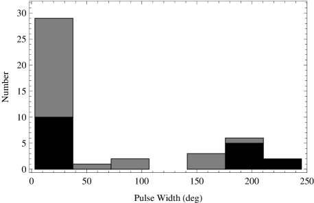
Figure 2: Frequency histograms of the $W_{10}$ (black) and $W_{50}$ (grey) pulsewidths for the interpulse pulsars listed by Weltevrede & Johnston (2008); the bars are stacked for clarity. It is evident that the data distributions can be treated as bimodal. Widths greater than $140\degr$ were assumed to have included the interpulses and were excluded from the $W_{10}$ and $W_{50}$ pulsewidth data sets used in this paper.

In a mean pulse profile the spacing between components usually increases, and with it the whole profile width, as the radio frequency, $f$, decreases. For instance, by measuring the profile widths of 6 pulsars up to 32 GHz, Xilouris et al. (1996) found that $W_{50}=b_{0}+b_{1}f^{-p}$ where $p$, $b_{0}$ and $b_{1}$ are constant for each pulsar, with $0.3<p<0.9$. The $W_{10}$ and $W_{50}$ pulsewidths tabulated in the ATNF catalogue are not all measured at the same observing frequency. The frequency dependence of the pulsewidth therefore introduces some statistical noise into the ‘ATNF Cat $W_{10}$’ and ‘ATNF Cat $W_{50}$’ data sets. As a consistency check, we have also examined the subsets consisting of only those pulsars whose catalogued pulsewidth values were measured in the Parkes Multibeam Survey at 1374 MHz (Manchester et al., 2001; Lorimer et al., 2006). These subsets are referred to hereafter as ‘Parkes MB $W_{10}$’ and ‘Parkes MB $W_{50}$’, and contain 377 and 934 pulsars respectively.

Both the $W_{10}$ and $W_{50}$ characteristic age–pulsewidth data distributions naturally lend themselves to binning in $\log{t_{c}}$, and it was also found numerically optimal to fit the mean pulsewidth, equation (36), as a function of $\log{t_{c}}$ rather than $t_{c}$, i.e. as $\left<{W}\right>\!(\log{t_{c}})$. The $W_{10}$ or $W_{50}$ data set is then binned to give $N$ data points, $\{\left(\overline{\log t_{c}}\right)_{i},\overline{W}_{i}\}$, $i=1,\ldots,N$. It is desirable to make the bins as narrow as possible in order to give maximum resolution in $\log{}t_{c}$. This is because if a bin $i$ extends over a large range of $\log{}t_{c}$ in a region where the underlying function, here $\left<{W}\right>\!(\log t_{c})$, has a significant slope, then a part of the uncertainty in the estimated value of the mean pulsewidth, $\overline{W}_{i}$, will result from the change in the underlying $\left<{W}\right>\!(\log{t_{c}})$ across the bin. On the other hand, it is desirable to include as many points as possible in a bin to reduce the uncertainty in the $\overline{W}_{i}$ estimate of $\left<{W}\right>\!\left[\left(\overline{\log t_{c}}\right)_{i}\right]$, and also to ensure that the errors in the estimates are approximately normally distributed so that standard data-analysis procedures can be applied. To attempt to balance these competing effects we binned the data so that each bin contained about 30 pulsars – the minimum number of points to ensure that the errors are approximately normally distributed.

Least-squares fittings are made to both the $W_{10}$ and $W_{50}$ data sets. Even though there are more data points in the $W_{50}$ than the $W_{10}$ data sets, the $W_{10}$ is superior for our pulsewidth fitting because the $W_{50}$ set suffers more from confusion. This is because a $W_{50}$ measurement will include outlying components in a profile only if they are above 50 per cent of the maximum intensity. A $W_{10}$ measurement is more likely to include the outlying components and so will give a more consistent estimate of the total pulsewidth. A histogram of the ratio of $W_{10}/W_{50}$ is found to be unimodal, with a peak at about 2. However, it extends to ratios above 10, demonstrating that the $W_{10}$ in those cases is detecting outlying emission missed by the $W_{50}$ measurement. The trade-off in relying on $W_{10}$ values is that the $W_{10}$ measurement is more difficult to make than the $W_{50}$, and so there are fewer pulsars with existing $W_{10}$ measurements.

The data sets considered in this paper are summarized in Table 1. For each data set it gives the name of the set and the number of pulsars it contains, and describes the binning of the data. Fig. 3 shows the ATNF Cat data sets and compares them to the corresponding Parkes MB data sets. We see that the ATNF Cat and Parkes MB data sets have very similar distributions with respect to characteristic age.

Table 1: Summary of the four data sets considered in this paper.

Dataset	Size	Binning
Parkes MB $W_{10}$	377	bins 1–13: 29 pulsars/bin
Parkes MB $W_{50}$	934	bins 1–14, 19–31: 30 pulsars/bin
		bins 15–18: 31 pulsars/bin
ATNF Cat $W_{10}$	872	bins 1–14, 17–29: 30 pulsars/bin
		bins 15–16: 31 pulsars/bin
ANTF Cat $W_{50}$	1420	bins 1–19, 30–47: 30 pulsars/bin
		bins 20–29: 31 pulsars/bin

Figure 3: Comparison of the four mean-pulsewidth data sets considered in this paper, as summarized in Table 1. The $W_{10}$ and $W_{50}$ ‘ATNF Cat’ data sets are shown in black (connected by a dashed black line), while the two corresponding ‘Parkes MB’ data sets are shown in grey (connected by a solid grey line). The error bars are 1$\sigma$ standard errors for the binned data.

4.2 Fitting procedure

Each model of initial alignment has four free parameters: $\rho_{\infty}$, $n_{\gamma}$, $\mu_{\gamma{},\log}$ and $\sigma_{\log}$. The aim is to determine these four parameters by least-squares fitting the model $\left<{W}\right>\!(\log{t_{c}})$-curve to the binned data. The mean pulsewidths, $\overline{W}_{i}$, computed for each bin $i$, have normally-distributed errors, and so the uncertainties for the fitted parameters can be found by computing the parameter covariance matrix, $s_{kl}$ (e.g. Press et al., 1992, Ch. 15). This matrix can in turn be used to compute a parameter correlation matrix, $r_{kl}$, for the parameter estimates.

Proceeding in this way it was found that least-squares estimates of the four parameters had large uncertainties, and hence were of questionable statistical merit. These large uncertainties were found to result mostly from a high correlation between the four parameters, with the off-diagonal values of the parameter correlation matrix all being around $\pm{}0.98$. Furthermore, very different sets of parameter values could give very similar fittings to the data.

To tackle these problems we fixed $n_{\gamma}$ at specific trial values, leaving three free parameters: $\rho_{\infty}$, $\mu_{\gamma,\log}$, and $\sigma_{\log}$. The cross-correlation between the parameters was significantly reduced. Correspondingly, the uncertainties in the parameters were also significantly reduced and, given the assumptions, provided statistically significant constraints. The reduced $\chi^{2}$ ($\chi^{2}_{\mathrm{red}}\equiv\chi^{2}/\mathrm{dof}$) for these three-parameter fits were then examined as a function of the pre-set parameter $n_{\gamma}$; a minimum in this function would indicate that a particular value of $n_{\gamma}$ was giving a superior fit. In that case a least-squares fit was computed by allowing all four parameters (including $n_{\gamma}$) to vary, and the solution was checked against the three-parameter fit for consistency.

We recall that the parameters $n_{\gamma}$ and $\mu_{\gamma,\log}$ are the values of $n$ and $\mu_{\log}$ assuming that $\gamma=1/2$. More generally, for fitted values of $n_{\gamma}$ and $\mu_{\gamma,\log}$, the relationships between different values $\gamma$, $n$ and $\mu_{\log}$ are found via equations (21) and (35) to be $n=2\gamma\left(n_{\gamma}-1\right)+1$, $\mu_{\log}=\mu_{\gamma,\log}-\log\left(2\gamma\right)$, and hence

$$\frac{n-1}{n_{\gamma}-1}=10^{\mu_{\gamma,\log}-\mu_{\log}}\mbox{~{}.}$$ (43)

4.3 Fits to the data

The three-parameter fits showed clear minima in $\chi^{2}_{\mathrm{red}}\left(n_{\gamma}\right)$ at $n_{\gamma}\approx{2.3}$ for all of the datasets, excluding the ATNF Cat $W_{50}$ data. For instance, Fig. 4 plots $\chi^{2}_{\mathrm{red}}\left(n_{\gamma}\right)$ for Models I, II and III fitted to the ATNF Cat $W_{10}$ data.

Figure 4: Plot of $\chi^{2}_{\mathrm{red}}$ as a function of $n_{\gamma}$, for each of the three models of initial alignment fitted to the ATNF Cat $W_{10}$ data: Model I (solid black), Model II (dashed), and Model III (dotted). Each model exhibits a minimum in $\chi^{2}_{\mathrm{red}}$ at $n_{\gamma}$ around 2.3.

Fig. 5 shows three-parameter fitted curves of $\left<{W}\right>\!\left(\log{t_{c}}\right)$ for Model II with $n_{\gamma}$ set at values between 1.5 and 4; equivalent plots for Models I and III are similar. In each case setting $n_{\gamma}$ to around 2.3 and least-squares fitting the other three parameters gives the best fit to the data, in particular at low characteristic age. Performing the same procedure with $n_{\gamma}$ higher or lower than this value results in a curve that goes to lower pulsewidth than the measured value at low $\log{t_{c}}$. The figure shows for the ATNF Cat $W_{50}$ data set that even though $\chi^{2}_{\mathrm{red}}$ does not have a clear minimum at $n_{\gamma}\approx{2.3}$, the $n_{\gamma}\approx{2.3}$ fit appears to best explain the low-$t_{c}$ mean $W_{50}$ pulsewidths.

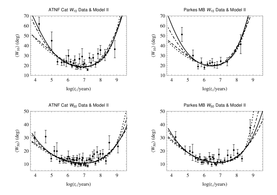
Figure 5: Mean pulsewidth, $\left<{W}\right>$, as a function of log characteristic age. The data sets are given in the title of each figure; they are the same as those plotted in Fig. 3 and are summarized in Table 1. Error bars are $1\sigma$ standard errors for the binned data. Mean angular pulsewidths for Model II are least-squares fitted to the binned data for each of the following values of $n_{\gamma}$: $n_{\gamma}=1.5$ (dashed), $n_{\gamma}=2.3$ (solid), $n_{\gamma}=3.0$ (dot-dashed), and $n_{\gamma}=4$ (dotted). The vertical scales are different for the $W_{10}$ and $W_{50}$ data sets. Note that for the Parkes MB $W_{50}$ data set, the Model II curves did not converge for $n_{\gamma}=1.5$ or $n_{\gamma}\geq{}4$. In that case, the dashed curve and the dotted curve represent $n_{\gamma}=1.7$ and 3.95 respectively. In each plot, except the ATNF Cat $W_{50}$ plot, the solid $n_{\gamma}=2.3$ curve is approximately the best-fitting curve to the data across the different values of $n_{\gamma}$, having the lowest value of $\chi^{2}_{\mathrm{red}}$. None of the curves in the ATNF Cat $W_{50}$ plot was clearly distinguished by a minimum in $\chi^{2}_{\mathrm{red}}$.

Table 2 gives the measured values of $n_{\mathrm{app}}$ for six pulsars (table 2, p. 1291, Livingstone et al., 2006, and references therein). The uncertainties in the last digit of $n_{\mathrm{app}}$ are shown, being 1$\sigma$ confidence intervals. The characteristic ages are also listed, indicating that these pulsars are all very young. Except for the Vela pulsar, the determinations of $n_{\mathrm{app}}$ were all made by standard timing analyses that obtained phase coherent solutions (Livingstone et al., 2007). This approach could not be used for the Vela pulsar because of its large glitches, so $\dot{\nu}$ was determined from data 150 days after each glitch and then extrapolated back to the glitch epoch; $\ddot{\nu}$ could then be determined from the change in $\dot{\nu}$ over time (Lyne et al., 1996).

It is noteworthy that the mean value of $n_{\mathrm{app}}$ in Table 2 is $2.42\pm{}0.05$, compared to the values of $n_{\gamma}\approx 2.3$ that give the best fits of the Candy-Blair models to the pulsewidth data. On the grounds of equation (25) we expect $n_{\mathrm{app}}\approx{}n_{\gamma}$ for $\gamma\approx 1/2$ and $t_{c}\ll\tau_{\gamma}$. Fig. 5 shows that the constraint of $n_{\gamma}\approx{}2.3$ is based primarily on young pulsars, but a much larger sample than the six given in Table 2.

Table 2: Measured values of the apparent braking index, $n_{\mathrm{app}}$.

Pulsar	$t_{c}\,$(yr)	$n_{\mathrm{app}}$	Reference
J1846-0258	723	$2.65(1)$	Livingstone et al. (2006)
B0531+21, Crab	1240	$2.51(1)$	Lyne et al. (1993)
B1509-58	1550	$2.839(3)$	Livingstone et al. (2005)
J1119-6127	1610	$2.91(5)$	Camilo et al. (2000)
B0540-69, LMC	1670	$2.140(9)$	Livingstone et al. (2005)
B0833-45, Vela	11300	$1.4(2)$	Lyne et al. (1996)

Table 3 gives the parameter values obtained from the three-parameter fits to the four data sets. The error ranges are $1\sigma$ confidence intervals, and the degrees of freedom (dof) for each data set are given. For each fitting the parameter $n_{\gamma}$ is fixed at the value at which $\chi^{2}_{\mathrm{red}}$ is minimum, except in the case of the ATNF Cat $W_{50}$ data where no clear minima were found, and so $n_{\gamma}$ was fixed at 2.3 for comparison with the other fits. For each data set, all three models predict similar $\mu_{\gamma,\log}$ and $\sigma_{\log}$ values. The only significant parameter difference between the three alignment models is the predicted limiting emission cone half-width, $\rho_{\infty}$. Fig. 6 shows curves of $\left<{W}\right>\!\left(\log{t_{c}}\right)$ for Models I, II and III using the parameter values listed inTable 3. It is evident that the pulsewidth data alone can not be used to distinguish between the three models of initial alignment.

Table 3: Three-parameter least-squares fits of Models I, II and III.

	$n_{\gamma}$	$\rho_{\infty}$ (deg)	$\mu_{\gamma,\log}$	$\sigma_{\log}$	${\chi^{2}_{\mathrm{red}}}$
ATNF Cat $W_{10}$ Fits $(\mathrm{dof}=26)$
I	2.47	$5.6\pm{0.2}$	$6.5\pm{0.2}$	$0.71\pm{0.08}$	1.73
II	2.30	$4.11\pm{0.12}$	$6.1\pm{0.2}$	$0.83\pm{0.08}$	1.74
III	2.25	$1.99\pm{0.08}$	$6.2\pm{0.3}$	$0.89\pm{0.08}$	1.72
ATNF Cat $W_{50}$ Fits $(\mathrm{dof}=44)$
$n_{\gamma}\equiv 2.3$ (no clear minimum in ${\chi^{2}_{\mathrm{red}}}$)
I	2.3	$2.78\pm 0.08$	$5.4\pm 0.3$	$1.02\pm 0.08$	1.47
II	2.3	$2.10\pm{0.07}$	$4.8\pm 0.4$	$1.20\pm 0.08$	1.46
III	2.3	$0.87\pm 0.04$	$5.1\pm 0.4$	$1.26\pm 0.09$	1.46
Parkes MB $W_{10}$ Fits $(\mathrm{dof}=10)$
I	2.19	$5.5\pm{0.3}$	$6.1\pm{0.4}$	$0.66\pm{0.13}$	1.05
II	2.30	$4.5\pm{0.2}$	$6.1\pm{0.4}$	$0.71\pm{0.14}$	1.18
III	2.05	$1.84\pm{0.15}$	$5.6\pm{0.5}$	$0.90\pm{0.14}$	1.16
Parkes MB $W_{50}$ Fits $(\mathrm{dof}=28)$
I	2.48	$3.33\pm{0.09}$	$6.1\pm{0.3}$	$0.83\pm{0.09}$	1.22
II	2.34	$2.36\pm{0.08}$	$5.3\pm{0.4}$	$1.08\pm{0.09}$	1.25
III	2.20	$0.87\pm{0.05}$	$5.1\pm{0.4}$	$1.21\pm{0.09}$	1.23

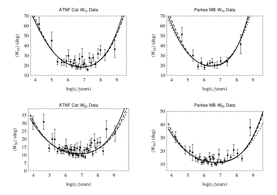
Figure 6: Mean pulsewidth, $\left<W\right>$, as a function of log characteristic age using the fitting parameters given in Table 3. Mean angular pulsewidths for Models I (dashed line), II (solid) and III (dotted) are least-squares fitted to the binned data.

The figures show that following a rapid decline in pulsewidth for young pulsars, there is a minimum in the pulsewidth for pulsars of moderate age followed by an increase for older pulsars: this is a clear signature of spin-magnetic alignment (CB83). The minimum occurs at $t_{c}\approx 10^{6.9}\,$yr in all three models for all data sets, except the Parkes MB $W_{10}$ data set where it occurs slightly earlier. The mean alignment time-scales obtained from the fitting process are around $10^{6}\,$yr which is less than previous estimates of around $10^{7}\,$yr. The log deviations of the time-scales range from 0.71 to 1.21, and are all larger than the value of 0.25 found by both CB86 and C93, which suggests that the more sensitive recent surveys have detected pulsars with a broader range of parameters.

As discussed near the end of Section 4.1, $W_{10}$ is superior to $W_{50}$ for pulsewidth fitting. Hence in the following we restrict our attention to the $W_{10}$ fits, in particular the ATNF Cat $W_{10}$ fit that was generated from a larger data set.

5 ANALYSIS AND IMPLICATIONS

5.1 Magnetic field decay model

As an alternative to magnetic alignment, many authors have proposed pulsar evolution through magnetic field decay. This will have a different effect on pulsewidth evolution. Suppose that the magnetic field decays exponentially, according to

$$B=B_{0}\exp(-t/\tau_{d})\,,$$ (44)

where $\tau_{d}$ is the field decay time-scale, and that $\alpha=\alpha_{0}$ remains constant (no alignment). Equation (5) for $P(t)$ still applies, so we still have equations (8) and (15) for $\rho(t)$ and $\rho(t_{c})$.

Fig. 7 shows curves of $\left<{W}\right>\!(\log{t_{c}})$ for a constant $\alpha=\alpha_{0}$ (using Models I, II and III for the $\alpha_{0}$ distribution) to illustrate the effect of magnetic field decay on pulsewidth evolution. The figure shows the same ATNF Cat $W_{10}$ binned data as before and the curves have been fitted assuming that $\log{\tau_{d}}$ has a normal distribution with mean $\mu_{d}$ and standard deviation $\sigma_{d}$. It was found necessary to fix $\sigma_{d}$ in order to get a convergent fit, and the small value of $\sigma_{d}=0.1$ was required in order to increase the size of $\mu_{d}$ to realistic values.

Qualitatively, the effect of field decay alone on pulsewidth evolution is a progressive decrease in pulsewidth over time, as seen in Fig. 7. The data do not support this evolution path: in contrast to the alignment models, the field decay model does not account for the increase in pulsewidth values for older pulsars.

From this work we cannot set an upper limit on the magnetic field decay rate. Clearly, weak magnetic-field decay could still occur concurrently with the alignment mechanism that causes the observed increase in pulsewidth for old pulsars. We can say that magnetic field decay is not the dominant evolutionary factor: both the $W_{50}$ and $W_{10}$ fits are consistent with magnetic field decay not being a significant factor in pulsar evolution. To model the combined effects of alignment and field decay is beyond the scope of this paper because of the relatively strong parameter cross-correlation that already exists in the alignment model alone.

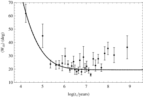
Figure 7: The mean angular pulsewidths obtained from the magnetic field decay model, as fitted to binned ATNF Cat $W_{10}$ data, are plotted against characteristic age. It has been assumed here that each pulsar has a constant inclination angle, $\alpha_{0}$, with the distribution of those angles determined by either Model I (dashed), II (solid) or III (dotted) of inclination angle as outlined in Section 3.3; the three curves are indistinguishable.

5.2 Inclination angle evolution

To investigate the question of the alignment of the magnetic and spin axes, Tauris & Manchester (1998) used the data sets of Rankin (1993b) and Gould (1994) that give estimates of $\alpha$ for a few hundred pulsars. These two datasets are derived using slightly different methods and assumptions, as is well summarized by Tauris & Manchester (1998). Tauris & Manchester binned each data set in $\alpha$ to examine the $\left<\log{t_{c}}\right>\!(\alpha)$ dependence. To these they fitted straight lines (their fig. 6, p. 632) in order to estimate the alignment time-scale, which they found to be around $10^{7}\,$yr.

Conversely, here the mean inclination angle associated with a log characteristic age is found by averaging the $\arcsin$ of equation (13), for $\sin\alpha$, over the $P(\alpha_{0})$ and $P(\log{\tau})$ distributions:

$$\left<\alpha\right>\!\left(\log{t_{c}}\right)=$$ (45)

$$\frac{1}{A}\int\limits_{0}^{\infty}\int\limits_{0}^{\pi/2}\alpha(\log{t_{c}})f_{b}f_{t}P(\alpha_{0})P(\log{\tau})\mathrm{d}\alpha_{0}\frac{\mathrm{d}\tau}{\tau}\mbox{.}$$

Using the fitted-parameter values found in Section 4 from the various pulsewidth data sets, the resulting $\left<\alpha\right>\!\left(\log{t_{c}}\right)$ curves for Models I, II and III are plotted in Fig. 8.

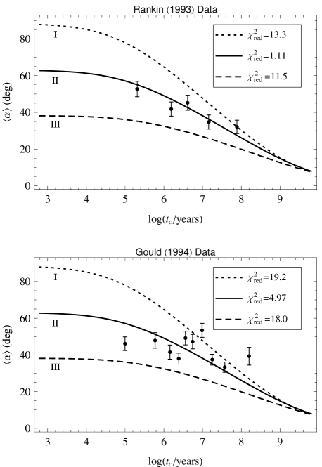
Figure 8: Mean angle of inclination, $\left<{\alpha}\right>$, as a function of log characteristic age. The data are determined from models of beam morphology and polarization data and are taken from the two references considered by Tauris & Manchester (1998). Binned data are shown with $1\sigma$ error bars, and exclude low-field (millisecond) pulsars having $B_{\mathrm{surf}}\leq 4\times{}10^{9}\,\mbox{G}$. The top figure shows the Rankin (1993b, tables 2 and 4–8) inclination angles for 148 pulsars; the central 3 bins each contain 30 points, while the first and last bins contain 29. The bottom figure shows the Gould (1994, tables 1–6) inclination angles for 301 pulsars; of the 10 bins, all contain 30 points, except the sixth bin which has 31. The plotted curves are $\left<\alpha\right>\!\left(\log{t_{c}}\right)$, equation (45), for each of the three models of initial alignment (I, II or III), using the parameter values determined from the best fits to the ATNF Cat $W_{10}$ data. The goodness-of-fit of the model curves to the binned data is measured using the reduced chi-squared statistic, $\chi^{2}_{\mathrm{red}}$, and the values for each curve are shown on the plots. Models I and III are seen to give a poor fit to both the Rankin and Gould mean inclination-angle data, while Model II gives a particularly good fit to the Rankin data.

Also plotted are the data from Rankin (1993b) and Gould (1994), in each case binned with about 30 points per bin. The error bars are $1\sigma$ standard errors computed from the binning. The actual errors in each of the $\alpha$ values are difficult to evaluate, since they depend on the validity of the underlying assumptions, as discussed by Manchester et al. (1998). As with the pulsewidth data, low-field (millisecond) pulsars having $B_{\mathrm{surf}}\leq 4\times{}10^{9}\,\mbox{G}$ have been removed from the data.

The model curves are compared with the binned data using the reduced chi-squared statistic, $\chi^{2}_{\mathrm{red}}$, which is shown for each model curve in Fig. 8. It was found that the inclination angle data are inconsistent with Models I and III, but compatible with Model II. Indeed Model II predicts the Rankin (1993b) data particularly well, with a ${\chi^{2}_{\mathrm{red}}}\sim{1}$.

5.3 Beaming fraction evolution

From equations (13) and (15) for $\sin\alpha(t_{c})$ and $\rho(t_{c})$, equation (30) for $f_{b}$ becomes

$$f_{b}\left(t_{c}\right)=\sin\alpha_{0}\left[1+{4t_{c}}/{(n-1)\tau}\right]^{-1/2}$$ (46)

$$\times\sin\left\{\rho_{\infty}\left[1+{(n-1)\tau}/{4t_{c}}\right]^{\gamma/(n-1)}\right\}\mbox{~{}.}$$

The mean beaming fraction as a function of characteristic age, $\left<{f_{b}}\right>(t_{c})$, is a key quantity in pulsar population studies. It is found by integrating $f_{b}\left(t_{c}\right)$ over the distribution functions $P(\alpha_{0})$ and $P(\log\tau)$. Using the parameter values from the best fit to the ATNF Cat $W_{10}$ data set, $\left<{f_{b}}\right>(t_{c})$ is plotted in Fig. 9 for the three initial alignment models.

Figure 9: (top) The mean beaming fraction, $\left<f_{b}\right>$, is plotted against log characteristic age for Models I, II and III, as labeled. (bottom) The scaled beaming fraction, $f_{b}/\sin\alpha_{0}$, is plotted against log characteristic age for Model II. The dashed curve has $\tau_{\gamma}=\mu_{\gamma,\log}$, the dot-dashed curve has $\tau_{\gamma}=\mu_{\gamma,\log}-\sigma_{\log}$, and the dotted curve has $\tau_{\gamma}=\mu_{\gamma,\log}+\sigma_{\log}$. For comparison, the corresponding Model II mean beaming fraction from the top plot is shown as a solid line. Both plots use the the ATNF Cat $W_{10}$ best-fitting parameters, Table 3.

Fig. 9 shows strong differences in the $\left<{f_{b}}\right>(t_{c})$ among the three models for young pulsars because of the differing initial conditions, with gradual reduction to similar values for older pulsars. The figure implies that the smallness of the observed sample size for old pulsars is significantly influenced by a low probability of observation. Because of completeness issues, and luminosity evolution uncertainty, we cannot evaluate the relative significance of beaming fraction evolution and pulsar ‘death’ (through reducing radio emission) in determining the number of observable old pulsars.

For individual pulsars, the beaming fraction evolution will depend on the pulsar’s $\alpha_{0}$ and $\tau_{\gamma}$ values, but the scaled beaming fraction ${f_{b}}(t_{c})/\sin\alpha_{0}$ is independent of $\alpha_{0}$. It is plotted in Fig. 9 for the Model II fit to the ATNF Cat $W_{10}$ data, using various values of $\tau_{\gamma}$. It is note-worthy that the scaled beaming fraction is considerably larger for pulsars with a longer alignment time-scale, and so these pulsars are more likely to be observed than those with a small alignment time-scale, even at young ages.

5.4 Alignment time-scales

From Table 3, the best-fitting mean log alignment time-scale, $\mu_{\gamma,\log}$, for Model II is found to be $6.1\pm{0.2}$ for the ATNF Cat $W_{10}$ fit, $6.1\pm{0.4}$ for the Parkes MB $W_{10}$ fit, and ${5.3\pm{0.4}}$ for the Parkes MB $W_{50}$ fit. The first and last of these three fits have the largest numbers of degrees of freedom, and they agree within two standard deviations of error. Furthermore, a spread in alignment time-scales is needed to accurately model the data (CB86), and for the three fits just mentioned, the standard deviations, $\sigma_{\log}$, are $0.83\pm{0.08}$, $0.71\pm{0.14}$ and $1.08\pm{0.09}$ respectively, indicative of quite a large spread in alignment time-scales about the means.

The mean time-scales quoted above are smaller than previous values obtained. The analyses of CB83, CB86 and C93 yielded a mean alignment time-scale of $2\times 10^{7}\,$yr. Other authors have argued in favour of magnetic alignment using different methods and obtained similar alignment time-scales of around $10^{7}\,$yr. See for examples Table 4: Lyne & Manchester (1988), Xu & Wu (1991), Kuz’min & Wu (1992) and Tauris & Manchester (1998) all used polarization data, while Weltevrede & Johnston (2008) used interpulse pulsar statistics.

Table 4: Alignment time-scales from different authors.

Authors	Alignment time-scale (yr)
CB83, CB86, C93	$2\times 10^{7}$
Lyne & Manchester (1988)	$10^{7}$
Xu & Wu (1991)	$1.5\times 10^{7}$
Kuz’min & Wu (1992)	$2\times 10^{7}$
Tauris & Manchester (1998)	$10^{7}$
Weltevrede & Johnston (2008)	$7\times 10^{7}$

From equation (35), the fitted value of $\mu_{\log}$ is determined by the fitted value of $\mu_{\gamma,\log}$ and the value of $\gamma$:

$$\mu_{\log}=\mu_{\gamma,\log}-\log\left({2\gamma}\right)\mbox{~{},}$$ (47)

as plotted in Fig. 10. We see that a mean alignment time-scale $10^{\mu_{\log}}\ga{}10^{7}\,$yr requires $\gamma>1$; that is inconsistent with previous findings that $\gamma$ is between $1/2$ and $2/3$. Conversely, for that range of $\gamma$-values, the curves in Fig. 10 give a mean alignment time-scale of around $10^{6}\,$yr.

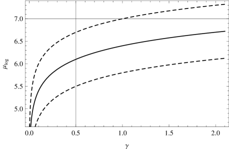
Figure 10: Plots of equation (47): the mean log alignment time-scale, $\mu_{\log}$, as a function of the parameter $\gamma$, which was introduced in equation (4). The solid curve corresponds to $\mu_{\gamma,\log}=6.1$ from the ATNF Cat $W_{10}$ Model II fit (Table 3), and the dashed curves are three standard deviations of error away from the black curve, $\mu_{\gamma,\log}=6.1\pm 0.6$. Previous studies have found a log alignment time-scale $\ga{}7$. This is inconsistent here with the empirical finding that $\gamma\approx{1/2}$.

5.5 Pulsar aging

Caution is required in using the characteristic age as a measure of the true ages of pulsars, as will now be explored. Defining $t_{\gamma}\equiv 2\gamma t$ and using equations (22) and (24) involving $\tau_{\gamma}$, it follows from equation (12) for $t(t_{c})$ that

$$t_{\gamma}\left(t_{c}\right)=\frac{\tau_{\gamma}}{2}\ln\left[1+\frac{4t_{c}}{\left(n_{\gamma}-1\right)\tau_{\gamma}}\right]\mbox{~{}.}$$ (48)

The mean log age, $\left<\log{t_{\gamma}}\right>$, as a function of the log characteristic age, $\log{t_{c}}$, is found by integrating over the distribution functions $P(\alpha_{0})$ and $P(\log{\tau})$. Consider the best fit to the ATNF Cat $W_{10}$ data having parameters as listed in Table 3. A plot of $\left<\log{t_{\gamma}}\right>\!(\log{t_{c}})$ for Model II is shown in Fig. 11; it shows that that $\left<\log{t_{\gamma}}\right>$ and $\log{t_{c}}$ agree up to $\log{t_{c}}\sim{}10\mu_{\gamma,\log}$, after which time $\left<\log{t_{\gamma}}\right>$ starts to fall below $\log{t_{c}}$. The curves for Models I and III are similar.

Figure 11: Plots of mean log age, $\left<\log{t_{\gamma}}\right>$, (solid curve) and log age, $\log{t_{\gamma}}$, (broken curves) as functions of log characteristic age for Model II: (dashed) $\tau_{\gamma}=\mu_{\gamma,\log}$, (dot-dashed) $\tau_{\gamma}=\mu_{\gamma,\log}-\sigma_{\log}$; and (dotted) $\tau_{\gamma}=\mu_{\gamma,\log}+\sigma_{\log}$. The parameters are from the best fit to the ATNF Cat $W_{10}$ data set (Table 3), and the straight line is $\log{t_{\gamma}}=\log{t_{c}}$.

However, the mean value $\left<\log{t}\right>\!(\log{t_{c}})$ applies to the population as a whole. For individual pulsars, the plots of $\log{t}(\log{t_{c}})$ depend on the value of $\tau_{\gamma}$ for that pulsar. Various tracks for individual pulsars are shown in Fig. 11: it is evident that in general the characteristic age diverges much more rapidly from the true age than for the populations mean ages, with the divergence being more rapid the smaller the alignment time-scale. Recall, however, that pulsars with shorter alignment time-scales have a smaller beaming fraction than those with longer time-scales, and so are less likely to be observed.

This highlights the uncertainty that may be present in previous studies that have used the characteristic age as a measure of true age when attempting to measure the alignment time-scales. The characteristic age can over-estimate the true age, and so will tend to give larger alignment time-scales if it is the time measure.

6 CONCLUSIONS

From Fig. 6, showing mean pulsewidths versus $\log{t_{c}}$, we have seen that the pulsewidth data clearly favour pulsar evolution through magnetic alignment, and not magnetic field decay alone nor progressive counter-alignment. There is a clear minimum of mean pulsewidth at about $t_{c}\approx 10^{6.9}\,$yr. The alignment process causes a significant increase in the mean $W_{10}$ pulsewidth for all characteristic age bins greater than $3\times 10^{7}\,$yr. This is particularly significant in view of the fact that the ATNF catalogue contains numerous pulsars with $t_{c}>10^{8}\,$yr, which were not available to the earlier studies.

The three models of initial alignment that were specified in Section 3.3 cannot be tested by fitting the Candy-Blair models to the pulsewidth data alone. However, once a Candy-Blair model has been fitted to the pulsewidth data, it can be used to predict mean inclination angle evolution, $\left<\alpha\right>\!(\log{t_{c}})$. Comparing these predictions to the datasets of Rankin (1993b) and Gould (1994), it was found that only Model II (a random initial inclination angle) gives a good fit to the data, as shown in Fig. 8.

The alignment time-scale found from fitting Model II to the ATNF Cat $W_{10}$ data (see Tables 1 and 3) is $10^{6.1}\,$yr, which is at least a factor of ten shorter than the timescales determined by a number of other authors (see Table 4). The fit requires that the log alignment time-scale varies with a standard deviation of about $0.83$ across the observed population. The fit gives a limiting cone opening half-angle of $4\aas@@fstack{\circ}11$, and a braking index parameter $n_{\gamma}$ of 2.30, consistent with the mean, $2.42\pm{}0.05$, of the measured apparent braking indices (equations (2) and (25), and Table 2). Consistent with empirical observations, the fit assumes the parameter $\gamma=1/2$ (see equation (4)). For other values of $\gamma$ the fitted parameters $n$ and $\mu_{\log}$ are determined from equations (21) and (35) respectively. A plot of the mean beaming fraction for this fit is given in Fig. 9.

The initial predictions of pulsar alignment due to electromagnetic braking (Davis & Goldstein, 1970; Michel & Goldwire, 1970) predicted time-scales of around $10^{3}$–$10^{4}\,$yr, which was rather small. The time-scales will be increased if pulsars are born with their magnetic and rotation axes nearly orthogonal. Jones (1976; 1976a; 1976b) found that the inclusion of a decreasing dissipative torque initially brought all pulsars close to counter-alignment, from which time the normal electromagnetic decay of $\alpha$ would begin. Jones predicted that the alignment phase started at around $10^{3}$–$10^{4}\,$yr, with a time-scale of around $10^{6}\,$yr, which was believed to be more in accord with the observed population.

We have found alignment time-scales consistent with the predictions of Jones, though with a significant spread in values, down to the time-scales consistent with the absence of the counter-alignment phase. Contrary to the model of Jones, though, we do not find evidence for all pulsars starting their alignment phase with $\alpha_{0}$ close to $90\degr$ (i.e. Model I). This interesting counter-point to the model of Jones deserves further investigation.

Appendix A PULSEWIDTH AVERAGING INTEGRAL

The integral that averages the pulsewidth over a random distribution of viewing angles can be evaluated analytically, as follows. As above, $\alpha$ is the pulsar magnetic-spin inclination angle, $\rho$ the emission cone half-width, and $\zeta$ is the angle between the observer’s direction and the pulsar’s spin axis.

A.1 Observer dependence of pulsewidth

For an individual pulsar, the variation of its observed angular pulsewidth with observer viewing angle is given by the formula (Manchester & Taylor, 1977, p. 218)

$$W(\alpha,\rho,\zeta)=2\arccos\left(\frac{\cos\rho-\cos\alpha\,\cos\zeta}{\sin\alpha\,\sin\zeta}\right)\,\mbox{,}$$ (49)

which is equation (26) in the main text above.

In considering the variation of $W$ with viewing angle, it is helpful to employ the variable $x\equiv\cos\zeta$. Equation (49) takes the form

$$W(\alpha,\rho,x)=2\arccos\!\left[f(x)\right]\,\mbox{,}$$ (50)

with the abbreviations

$$f(x)\equiv\frac{1}{\sin\alpha}\frac{b-ax\;}{(1-x^{2})^{1/2}}\;\mbox{,~{}}a\equiv\cos\alpha\;\mbox{,~{}and~{}}b\equiv\cos\rho\;\mbox{.}$$ (51)

Note that

$$(\sin\alpha)\,f^{\prime}(x) = (bx-a)/(1-x^{2})^{3/2}\quad\mbox{and}$$ (52)

$$(\sin\alpha)\,f^{\prime\prime}(x) = (b-3ax+2bx^{2})/(1-x^{2})^{5/2}\;\mbox{.}$$ (53)

The function $f(x)$, which is just the cosine of the pulse angular half-width, is $<1$ throughout the cut across the emission beam by the sight line to any ‘illuminated’ observer. It reaches $1$ in magnitude (i.e. $f^{2}=1$) at the pulse visibility limits $\zeta=|\,\alpha\mp\rho\,|$, corresponding to $x=x_{\pm}$, where

$$x_{\pm} \equiv \cos(\alpha\mp\rho)=ab\pm\Delta\hskip 11.38109pt{\mbox{with}}$$ (54)

$$\Delta \equiv (1-a^{2})^{1/2}(1-b^{2})^{1/2}\;\mbox{.}$$ (55)

Substituting (54) into (51) gives

$$f(x_{\pm})=\frac{b{}(1-a^{2})^{1/2}\mp a{}(1-b^{2})^{1/2}}{[1-(ab\pm\Delta)^{2}]^{1/2}}\;\mbox{.}$$ (56)

This shows that at $x_{-}$, the ‘outer’ visibility limit, $f$ is always positive, i.e. $+1$. At $x_{+}$, the ‘inner’ visibility limit, $f$ is $+1$ for $\alpha>\rho$, $0$ for $\alpha=\rho$, and $-1$ for $\rho>\alpha$. Let’s visualize these three cases in turn.

(1) For $\alpha>\rho$, the visibility limits $x_{\pm}$ both correspond to zero pulsewidth, $W(x)=0$. Equations (52) and (53) show that the minimum value $(b^{2}-a^{2})^{1/2}/(\sin\alpha)$ of $f(x)$ – corresponding to the greatest pulsewidth – occurs for the cone of observers at $x=a/b$:

$$W_{\mathrm{max}}=2\arccos\left\{\left[\,1-(\sin\rho)^{2}/(\sin\alpha)^{2}\,\right]^{1/2}\right\}$$ (57)

at $\cos\zeta=(\cos\alpha)/(\cos\rho)$.

(2) For $\alpha=\rho$, one can visualize the emission cone as rolling around the spin axis, which is then the inner visibility limit. In this case, $f(x)=(\cot\alpha)[(1-x)/(1+x)]^{1/2}$; also $x_{+}=+1$ (observer looking along the spin axis) so $f(x_{+})=0$, corresponding to $W(x_{+})=\pi$. So $W(x)$ increases monotonically from $0$ at the outer visibility limit to $\pi$ on the spin axis in this special case.

(3) For $\rho>\alpha$, the beam will be ‘always on’ (unpulsed) to observers within $(\rho-\alpha)$ of the spin axis. So the pulse visibility limit $x_{+}$ then corresponds to $W=2\pi$, with $f(x)$ ranging from $+1$ at $x_{-}$ to $-1$ at $x_{+}$, with no minimum: $W(x)$ increases monotonically from $0$ at the outer visibility limit to $2\pi$ at the inner one.

A.2 Evaluating the averaging integral

Integrating equation (49) for $W(\alpha,\rho,\zeta)$ over a random distribution of viewing angles, using the observer distribution function $(\sin\zeta)/(2f_{b})$, gives the mean angular pulsewidth, for pulsars of given $\alpha$ and $\rho$:

$$\left<{W}\right>\!(\alpha,\rho) = (2f_{b})^{-1}\int_{|\alpha-\rho|}^{\alpha+\rho}W(\rho,\alpha,\zeta)\sin\zeta\,\mathrm{d}\zeta$$ (58)

$$= f_{b}{{}^{-1}}\int_{x_{-}}^{x_{+}}\arccos\!\left[f(x)\right]\,\mathrm{d}x\;.$$ (59)

It is integration of the observer distribution function $(\sin\zeta)/2$ over the same range that yields the beaming factor $f_{b}=\sin\alpha\,\sin\rho$.

Note for use below that

$$(\sin\alpha)\left[1-f^{2}(x)\right]^{1/2} = G^{1/2}(x)/(1-x^{2})^{1/2}\;\mbox{,}$$ (60)

$$\mbox{with~{}~{}}G(x) \equiv (x-x_{-})(x_{+}-x)\;\mbox{.}$$ (61)

The function $G(x)$ describes an inverted parabola: it is zero at the limits of integration $x_{\pm}$ and positive in between, with a maximum value $(1-a^{2})(1-b^{2})=\sin^{2}\alpha\,\sin^{2}\rho\;(=f_{b}{{}^{2}})$ at $x=ab=\cos\alpha\,\cos\rho$.

Applying integration by parts in equation (59) for $\left<{W}\right>$ reduces the problem to one of evaluating an integral of an algebraic function. Using $\mathrm{d}({\arccos}X)=-(1-X^{2})^{-1/2}\mathrm{d}X$ together with equations (52) and (60) for $\mathrm{d}f/\mathrm{d}x$ and $(1-f^{2})^{1/2}$ gives

$$\left<{W}\right>\!(\alpha,\rho)f_{b} = x_{+}\arccos\!\left[f(x_{+})\right]$$ (62)

$${}+{}\int_{x_{-}}^{x_{+}}\frac{x(bx-a)\;\mathrm{d}x}{(1-x^{2})G^{1/2}(x)}\;\mbox{,}$$

because the integrated part $x\arccos\!\left[f(x)\right]$ – which by equation (50) is just $x\,W(x)/2$ – always vanishes at the limit $x_{-}$, where $f=+1$ always. The first term on the RHS of equation (62) is

$$\begin{array}[]{rccl}0&\mbox{for}&\alpha>\rho&[f(x_{+})=+1]\mbox{~{},}\\ \pi/2&\mbox{for}&\alpha=\rho&[f(x_{+})=0\;\mbox{,~{}}x_{+}=+1]\mbox{~{},}\\ \pi\cos(\rho-\alpha)&\mbox{for}&\alpha<\rho&[f(x_{+})=-1]\mbox{~{}.}\end{array}$$ (63)

Re-arranging the integrand in equation (62) gives

$$\left<{W}\right>\!(\alpha,\rho)f_{b}=\frac{x_{+}}{2}W(x_{+})$$ (64)

$${}+{}\int_{x_{-}}^{x_{+}}\left(\frac{b-a}{2(1-x)}+\frac{b+a}{2(1+x)}-b\right)\frac{\mathrm{d}x}{G^{1/2}(x)}\;\mbox{.}$$

This result shows that we can employ the following indefinite integrals, in which $\Delta$ and $G$ are defined by equations (55) and (61):

$$\int G^{-1/2}(x)\,\mathrm{d}x=\arcsin\!\left[(x-ab)/\Delta\right]{\mbox{~{}and}}$$ (65)

$$\int\frac{\mathrm{d}x}{(1\pm x)G^{1/2}(x)}=\int\frac{\mathrm{d}x}{(1\pm x)\left[(x-x_{-})(x_{+}-x)\right]^{1/2}}$$ (66)

$$= \frac{2}{|\,a\pm b\,|}\arctan\sqrt{\frac{(x-x_{-})(1\pm x_{+})}{(x_{+}-x)(1\pm x_{-})}}\;\;\mbox{,}$$

where $x_{\pm}=ab\pm\Delta$ and equation (55) for $\Delta$ have been used.

So the required definite integrals are

$$\int_{x_{-}}^{x_{+}}G^{-1/2}(x)\,\mathrm{d}x = \pi\mbox{~{},~{}~{}and}$$ (67)

$$\int_{x_{-}}^{x_{+}}\frac{\mathrm{d}x}{(1\pm x)G^{1/2}(x)} = \frac{\pi}{\,|a\pm b\,|}\;\mbox{.}$$ (68)

Thanks to these definite integrals, equation (64) for the observer-averaged pulsewidth evaluates to

$$\left<{W}\right>\!(\alpha,\rho)f_{b}=\frac{x_{+}}{2}W(x_{+})+\frac{\pi}{2}[\,{\mathrm{sign}}(b-a)+1-2b\,]\;\mbox{.}$$ (69)

That is:

$$\left<{W}\right>\!(\alpha,\rho)f_{b}=$$ (72)

$$\left\{\begin{array}[]{rll}\left[\,1-\cos\rho\,\right]\pi&\mbox{for}&\alpha\geq\rho\;\mbox{,}\\ \left[\,\cos(\rho-\alpha)-\cos\rho\,\right]\pi&\mbox{for}&\alpha\leq\rho\;\mbox{,}\\ \end{array}\right.$$

as used in the main text – equation (38) above.

References

- Beskin et al. (1984) Beskin V. S., Gurevich A. V., Istomin Y. N., 1984, Ap&SS, 102, 301
- Camilo et al. (2000) Camilo F., Kaspi V. M., Lyne A. G., Manchester R. N., Bell J. F., D’Amico N., McKay N. P. F., Crawford F., 2000, ApJ, 541, 367
- Candy (1993) Candy B. N., 1993, PhD thesis, University of Western Australia
- Candy & Blair (1983) Candy B. N., Blair D. G., 1983, MNRAS, 205, 281
- Candy & Blair (1986) Candy B. N., Blair D. G., 1986, ApJ, 307, 535
- Davis & Goldstein (1970) Davis L., Goldstein M., 1970, ApJ, 159, L81
- Gil & Han (1996) Gil J. A., Han J. L., 1996, ApJ, 458, 265
- Gould (1994) Gould D. M., 1994, PhD thesis, The University of Manchester
- Gunn & Ostriker (1970) Gunn J. E., Ostriker J. P., 1970, ApJ, 160, 979
- Johnston & Galloway (1999) Johnston S., Galloway D., 1999, MNRAS, 306, L50
- Jones (1976a) Jones P. B., 1976a, Nature, 262, 120
- Jones (1976b) Jones P. B., 1976b, ApJ, 209, 602
- Jones (1976) Jones P. B., 1976, Ap&SS, 45, 369
- Kuz’min & Wu (1992) Kuz’min A. D., Wu X., 1992, Ap&SS, 190, 209
- Livingstone et al. (2005) Livingstone M. A., Kaspi V. M., Gavriil F. P., 2005, ApJ, 633, 1095
- Livingstone et al. (2005) Livingstone M. A., Kaspi V. M., Gavriil F. P., Manchester R. N., 2005, ApJ, 619, 1046
- Livingstone et al. (2007) Livingstone M. A., Kaspi V. M., Gavriil F. P., Manchester R. N., Gotthelf E. V. G., Kuiper L., 2007, Ap&SS, 308, 317
- Livingstone et al. (2006) Livingstone M. A., Kaspi V. M., Gotthelf E. V., Kuiper L., 2006, ApJ, 647, 1286
- Lorimer et al. (2006) Lorimer D. R., Faulkner A. J., Lyne A. G., Manchester R. N., Kramer M., McLaughlin M. A., Hobbs G., Possenti A., Stairs I. H., Camilo F., Burgay M., D’Amico N., Corongiu A., Crawford F., 2006, MNRAS, 372, 777
- Lyne & Manchester (1988) Lyne A. G., Manchester R. N., 1988, MNRAS, 234, 477
- Lyne et al. (1996) Lyne A. G., Pritchard R. S., Graham-Smith F., Camilo F., 1996, Nature, 381, 497
- Lyne et al. (1993) Lyne A. G., Pritchard R. S., Smith F. G., 1993, MNRAS, 265, 1003
- Lyne & Smith (2006) Lyne A. G., Smith F. G., 2006, Pulsar Astronomy, 3rd ed.. Cambridge University Press, Cambridge
- Manchester et al. (1998) Manchester R. N., Han J. L., Qiao G. J., 1998, MNRAS, 295, 280
- Manchester et al. (2005) Manchester R. N., Hobbs G. B., Teoh A., Hobbs M., 2005, AJ, 129, 1993
- Manchester et al. (2001) Manchester R. N., Lyne A. G., Camilo F., Bell J. F., Kaspi V. M., D’Amico N., McKay N. P. F., Crawford F., Stairs I. H., Possenti A., Morris D. J., Sheppard D. C., 2001, MNRAS, 328, 17
- Manchester & Taylor (1977) Manchester R. N., Taylor J. H., 1977, Pulsars. Freeman, San Francisco
- Manchester & Taylor (1981) Manchester R. N., Taylor J. H., 1981, AJ, 86, 1953
- McKinnon (1993) McKinnon M. M., 1993, ApJ, 413, 317
- Michel & Goldwire (1970) Michel F. C., Goldwire Jr. H. C., 1970, Astrophys. Lett., 5, 21
- Narayan & Ostriker (1990) Narayan R., Ostriker J. P., 1990, ApJ, 352, 222
- Pandey & Prasad (1996) Pandey U. S., Prasad S. S., 1996, A&A, 308, 507
- Phinney & Blandford (1981) Phinney E. S., Blandford R. D., 1981, MNRAS, 194, 137
- Press et al. (1992) Press W. H., Teukolsky S. A., Vetterling W. T., Flannery B. P., 1992, Numerical Recipes: The Art of Scientific Computing, 2nd edition. Cambridge University Press, Cambridge
- Rankin (1993a) Rankin J. M., 1993a, ApJ, 405, 285
- Rankin (1993b) Rankin J. M., 1993b, ApJS, 85, 145
- Ruderman & Sutherland (1975) Ruderman M. A., Sutherland P. G., 1975, ApJ, 196, 51
- Tauris & Konar (2001) Tauris T. M., Konar S., 2001, A&A, 376, 543