Search for Scalar Diquarks at the LHeC Based Gamma-Proton Collider
Abstract
The diquark exotics which couple to a pair of quarks are predicted by the Compositeness and Superstring inspired model. We study the single production of scalar diquarks at LHeC based collider options. The background for three jet final states are examined through appropriate kinematical cuts. We discuss the possibility of measurements for the charges of scalar diquarks ( and ).
1. Introduction
Diquarks are suggested by the models beyond the Standard Model (SM), such as the superstring-inspired models [1] and composite models [2]. Diquarks have scalar and vector form and carry baryon number , and no lepton number. They carry electric charges , or .
Diquark production was examined in hadron colliders [3, 4, 5, 6, 7, 8, 9], [6, 10] and colliders [6, 11]. The collider dedector at Fermilab (CDF) has set limits on the masses of scalar diquarks (predicted by model) decaying to dijets with the exclusion of mass range GeV [3]. This limit is expected to be approximately valid for other scalar diquarks. There is also indirect bounds imposed on couplings by the electroweak precision data from LEP where these bounds allow diquark-quark cuplings up to a value = [12].
In this work, we analysed single production of scalar diquarks in a LHeC based collider. Interaction Lagrangian and quantum numers of scalar diquarks are examined to calculate the decay widths, differential cross sections and total cross sections of the signal, and the corresponding background. The signal and bacground analysis are performed for the scalar diquarks of , and types. The main parameters of the energy and luminosity options for a LHeC based collider are listed in table (1).
| Collider | (TeV) | (TeV) | (TeV) | ||
|---|---|---|---|---|---|
| LHeC | 0.07 | 7 | 1.40 | 1.28 | 10-100 |
| LHeC | 0.14 | 7 | 1.98 | 1.80 | 10-100 |
2. Interaction Lagrangian
Model independent, baryon number conserving, general invariant effective lagrangian for scalar and vector diquarks has the form [4, 5]
| (1) |
In Eq. (1), denotes the left-handed quark spinor and is the charge conjugated quark field. For the sake of simplicity, color and generation indices are ommitted in (1). Scalar diquarks , , are singlets and is a triplet. Vector diquarks and are doublets. At this stage, we assume that each SM generation has its own diquarks and relevant couplings in order to avoid flavour changing neutral currents. A general classification of the first generation, color anti-triplet diquarks is shown in table 1 [6].
| SU(3)C | SU(2)W | U(1)Y | Couplings | ||
| Scalar Diquarks | |||||
| 3⋆ | 1 | 2/3 | 1/3 | ||
| 3⋆ | 1 | -4/3 | 2/3 | ||
| 3⋆ | 1 | 8/3 | 4/3 | ||
| 3⋆ | 3 | 2/3 | |||
| Vector Diquarks | |||||
| 3⋆ | 2 | -1/3 | |||
| 3⋆ | 2 | 5/3 |
We consider the color scalar or diquarks coupled to pairs, or diquarks coupled to pair and or diquarks coupled to pair. Here, denotes the isospin triplet component of scalar diquarks. Diquark interactions with the gauge bosons are given as
| (2) |
where covariant derivative is where , , and denote photon, - boson, boson and gluon fields, respectively. is the electromagnetic charge of a given diquark and is the weak charge, the third component of the weak isospin and is the Weinberg angle, is the strong coupling constant and are the Gell-Mann matrices.
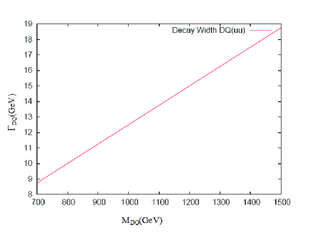
The decay widths () for scalar diquark is calculated from the equation (1) and we plot the diquark decay width versus diquark mass in fig. 1.
3. Production Cross Section for Scalar Diquarks
Scalar diquarks can be produced singly via the subprocess and the differential cross section is given by
| (3) |
where and are Mandelstam variables for the subprocess . and are the charges of initial and final quarks, respectively. As it can be seen from equation (3), the cross section is proportional to diquark charges. Therefore, the diquark charges can be identified at a LHeC based p collider. In figure 2, the hadronic process for diquark single production is shown.

The signal for diquark single production would clearly manifest itself in three jets cross sections. The total cross section for the single production of diquarks at p collider is given by
| (4) |
where is the quark distribution functions from the proton. The third integration over is taken in the interval and , where and . The energy spectrum of the Compton backscattered photons from electrons is given by
| (5) |
with
| (6) |
where and is the ratio of the backscattered photon energy to the initial electron energy. The energy of converted photons restricted by the condition . The value corresponds to as given in [13].
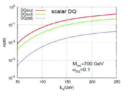
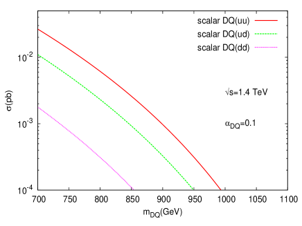
In figure 3, total cross sections for scalar diquarks depending on the electron beam energies are shown. From these plots we see the high energy and low energy behaviour of the total cross section for a given value of and . The total cross sections have no divergencies at large energies. Thus, equation (4) prove the unitarity condition. In figure (4), the total cross sections versus scalar diquark masses are plotted for the LHeC ( TeV) energy with the coupling using CTEQ parton distribution functions [14] at the factorization scale . From these figures we find that diquarks with charge have the largest cross sections when compared to the other types.
4. Signal and Background
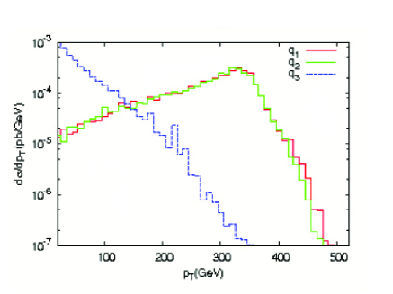
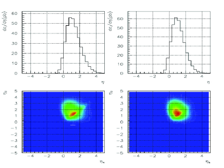
We generate diquark signal and the corresponding background events with the program CalcHEP [15]. Here, we consider two types of background one is interfering with the signal events and the other is reducible background contributing to three-jet events. The background for three-jet events have large cross sections, since the signal has different shape than the background, still we have opportunity to reduce these backgrounds by applying suitable kinematical cuts. In figure (5), the distribution of 3 jets for signal with GeV are shown. The jets from diquarks have large transverse momentum distribution around the half value of the diquark mass. Thus, we need at least 20 GeV for the transverse momentum cut and additional kinematics variables to reduce background more efficiently. In figure (6), the pseudo-rapidity distribution for signal with GeV and background are shown at LHeC with TeV.
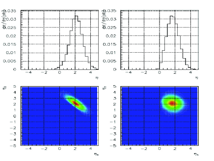
From figure (6), signal jets from scalar diquark are mostly located in the pseudo-rapidity () region . In figure (7), one can see the distribution of pseudo-rapidity (mostly in the range ) from SM three-jet background at LHeC with TeV. The invariant mass distribution of dijets from the scalar diquark signal and the SM background are shown in figure (8).
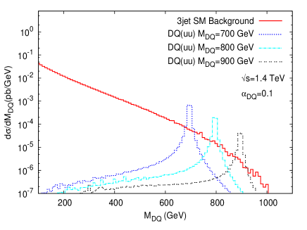
From these figures, more appropriate cuts for signal jets are , , GeV at LHeC TeV energy option. Same calculations have been performed for LHeC TeV energy option. In this case, the appropriate cuts for signal jets has been founded as , , GeV at LHeC TeV energy option.
In order to obtain the observability of diquarks at LHeC based gamma-p collider we have calculated the signal (S) and background (B) event estimations for an integrated luminosity of for one year of operation. The signal generated by a diquark of mass and decay rate is calculated integrating the differential cross section in the two-jet invariant mass interval which gives approximately of the events around the resonance. For a realistic analysis of the background events we take into account the finite energy resolution of the generic hadronic calorimeter as for jets with . The corresponding two-jet invariant mass resolution is given approximately by . The background is calculated by integrating the cross sections in the range with . The significance of signal over the background is defined as . Thus we used appropriate cuts and the dedector parameters to find the observability of diquarks at LHeC based collider. Then, we listed the values in table (3) and (4) where SS represent significance of diquarks.
| for | |||
| (GeV) | |||
| 700 | 17.2 | 3.6 | 1.2 |
| 800 | 10.1 | 1.8 | — |
| 900 | 4.8 | — | — |
| for | |||
| (GeV) | |||
| 700 | 36.4 | 10.8 | 3.6 |
| 800 | 28.3 | 7.8 | 2.5 |
| 900 | 19.9 | 5.1 | 1.6 |
| 1000 | 14.9 | 3.4 | 1.0 |
| 1100 | 10.4 | 2.1 | — |
| 1200 | 6.3 | — | — |
If we take at least signal events and as observability criteria, For the diquarks with charge it is possible to cover mass ranges up to TeV at the LHeC with and TeV. The scalar diquarks with charge can be observed up to TeV at TeV.
5. Conclusion
If diquarks exist, LHC could find them in resonance channel, however their charges and coupling types can be identified at a LHeC based collider. Up to 1.2 TeV mass of diquarks can be studied at LHeC based collider. In the single production mechanism, the spin of the diquarks can also be determined by studying the angular distributions of the final state jets with high .
Acknowledgements
This work is supported in part by the Turkish Atomic Energy Authority (TAEK) and the State Planning Organization (DPT) with grant number DPT2006K-120470.
References
-
[1]
J. L. Hewett and T. G. Rizzo, Phys. Rep., 183, 193, 1989.
-
[2]
H. Terazawa, Phys. Rev. D22, 184, 1980.
-
[3]
CDF Collaboration, CDF note 9246,2008.
-
[4]
S. Atag, O. Cakir, and S. Sultansoy,Phys. Rev., D59, 015008, 1999.
-
[5]
E. Arik, S. A. Cetin, O. Cakir and S. Sultansoy, J. High
Energy Phys., 09, 024, 2002.
-
[6]
O. Cakir, and M. Sahin, Phys. Rev., D72, 115011, 2005.
-
[7]
R.N.Mohapatra, Nobuchika Okada, and Hai-Bo
Yu, Phys.Rev. D 77, 01170(R), 2008.
-
[8]
M. Sahin, and O. Cakir, Balkan Physics Letters (BPL), 16(1), pp. 120-125, 161020 (2009).
-
[9]
Tao Han, Ian Lewis, and Thomas McElmurry, arXiv:0909.2666v1 [hep-ph] 15 Sep 2009.
-
[10]
A. Gusso, J. Phys. G:Nucl. Part. Phys. 30 (2004) 691-702.
-
[11]
T.G. Rizzo, Z.Phys. C 43, 223, 1989.
-
[12]
G. Bhattacharyya, D. Choudury and K. Sridhar,Phys. Lett., B355,193, 1995.
-
[13]
G. Bhattacharyya, D. Choudury and K. Sridhar,Phys. Lett., B355,193, 1995.
- [14] CTEQ Collaboration, H.L. Lai et al., Eur.Phys. J.C12 (2000) 375.
-
[15]
A.Pukhov et al.,hep-ph/9908288; A. Pukhov, e-Print Archive, hep-ph/0412191, 2004.
-
[16]
B. Schrempp, MPI-PAE/PTh, 72-86, 1986.; W. Buchmuller, Acta Phys. Austriaca,27, 517,1985
-
[17]
H. L. Lai et al. (CTEQ Collaboration), Eur. Phys. J., C 12, 375, 2000.
-
[18]
ATLAS Collaboration, Report No. ATLAS TDR 14,
CERN/LHCC 99-14, 1999; Report No. ATLAS TDR 15, CERN/LHCC 99-15,
1999.