The X-ray Energy Dependence of the Relation between Optical and X-ray Emission in Quasars
Abstract
We develop a new approach to the well-studied anti-correlation between the optical-to-X-ray spectral index, , and the monochromatic optical luminosity, . By cross-correlating the SDSS DR5 quasar catalog with the XMM-Newton archive, we create a sample of 327 quasars with X-ray S/N 6, where both optical and X-ray spectra are available. This allows to be defined at arbitrary frequencies, rather than the standard 2500 Å and 2 keV. We find that while the choice of optical wavelength does not strongly influence the relation, the slope of the relation does depend on the choice of X-ray energy. The slope of the relation becomes steeper when is defined at low ( 1 keV) X-ray energies. This change is significant when compared to the slope predicted by a decrease in the baseline over which is defined. The slopes are also marginally flatter than predicted at high ( 10 keV) X-ray energies. Partial correlation tests show that while the primary driver of is , the Eddington ratio correlates strongly with when is taken into account, so accretion rate may help explain these results. We combine the and -Lbol/LEdd relations to naturally explain two results: 1) the existence of the relation as reported in Young et al. (2009) and 2) the lack of a relation. The consistency of the optical/X-ray correlations establishes a more complete framework for understanding the relation between quasar emission mechanisms. We also discuss two correlations with the hard X-ray bolometric correction, which we show correlates with both and Eddington ratio. This confirms that an increase in accretion rate correlates with a decrease in the fraction of up-scattered disk photons.
1 Introduction
Optical/UV and X-ray continua in quasars are thought to originate in two physically distinct, but nevertheless related regions. The optical/UV spectrum is dominated by a ‘Big Blue Bump’ continuum feature (e.g., Elvis et al., 1994), most likely from thermal emission arising from an accretion disk (Shields et al., 1978; Malkan & Sargent, 1982; Ward et al., 1987). A hot gas lying above the disk in some unknown geometry then up-scatters these disk photons to form a hard power-law ( -1) (e.g., Mateos et al., 2005; Mainieri et al., 2007) in the X-ray spectrum (Haardt & Maraschi, 1991; Zdziarski et al., 2000; Kawaguchi et al., 2001).
While the shapes of the optical and X-ray continua are well known, the connecting continuum in the extreme ultraviolet (EUV) is not, because of absorption from our own galaxy. The EUV and soft X-rays form the ionizing continuum (h 13.6 eV) needed to ionize a quasar’s characteristic broad lines. The ionizing continuum is also responsible for any line-driven outflows from the accretion disk (Proga, 2007). Since direct observation of this continuum is not possible, it is often parameterized by an imaginary power-law with spectral index running from 2500 Å to 2 keV in the rest frame.
The importance of the ionizing continuum motivates the decades long study of the anti-correlation between and L2500 (Avni & Tananbaum, 1982; Kriss & Canazares, 1985; Tananbaum et al., 1986; Anderson & Margon, 1987; Wilkes et al., 1994; Pickering et al., 1994; Avni, Worrall & Margon, 1995); however, controversy continues. While some studies have found that depends primarily on redshift rather than optical luminosity (Bechtold et al., 2003; Kelly et al., 2007), others have suggested that may be entirely independent of redshift and optical luminosity (Yuan et al., 1998; Tang et al., 2007), arguing that if the dispersion in L2500 is much greater than the dispersion in L2keV, an apparent but artificial correlation will result. A narrow range in optical luminosity will enhance this effect.
In recent years, studies of the relation have become more comprehensive, with higher X-ray detection rates and largely complete samples that span a wide range of luminosities (Vignali et al., 2003; Strateva et al., 2005; Steffen et al., 2006; Just et al., 2007). For example, Steffen et al. (2006) work spans five and four decades in UV and X-ray luminosity, respectively, which helps minimize the effect of an artificial correlation due to selection effects. In addition, Strateva et al. (2005) estimated the dispersion in L2500 and L2keV, finding that the difference in dispersions was not enough to artificially reproduce a correlation. These studies used partial correlation analysis to conclude that the z correlation is insignificant, while the anti-correlation is highly significant. However, while the significance of the relation continues to be better understood, little is known of the underlying physics. Current disk-corona models (Beloborodov, 1999; Zdziarski et al., 1999; Nayakshin, 2000; Malzac, 2001; Sobolewska et al., 2004a, b) do not directly predict the relation.
Previous studies of the relation have largely lacked spectral slopes in the X-rays, and so used the traditional endpoints of 2500 Å and 2 keV, where an X-ray spectral slope ( 2, where = - + 1 for F) is assumed in order to obtain the X-ray flux at 2 keV. A systematic study with both optical and X-ray spectra enables an investigation of the relation at different frequencies than those traditionally used, revealing clues about the relation’s physical underpinnings.
The sample selection and measurement of are described in §2, and results of the data analysis are given in §3. Section 4 discusses the results, specifically their connection to other optical/X-ray relations found for quasars. We assume a standard cosmology throughout the paper, where H0 = 70 km s-1 Mpc-1, , and (Spergel et al., 2003).
2 The Sample
We have cross-correlated the DR5 Sloan Digital Sky Survey (SDSS) with XMM-Newton archival observations to obtain 792 X-ray observations of SDSS quasars. This gives the largest sample of optically selected quasars with both optical and X-ray spectra (473 quasars with X-ray S/N 6). Young et al. (2009) describes the SDSS quasar selection and cross-correlation with the XMM-Newton archive, as well as the X-ray data reduction and spectral fitting. For the purposes of this paper, we exclude broad absorption line (BAL) and radio-loud (RL) quasars, as these are known to have different distributions than typical, radio-quiet (RQ) quasars (Green & Mathur, 1996; Young et al., 2009). While Young et al. (2009) used an incomplete BAL list (Shen et al., 2008), this paper updates the BAL classification using the DR5 BAL catalog (Gibson et al., 2009). A total of 18 sources are re-classified as BALs, and an additional 15 sources are re-classified as non-BALs. A net result of three additional BALs, gives the SDSS/XMM-Newton Quasar Survey 55 BALs in total.
Since the goal is to use our knowledge of the X-ray spectrum to determine the effects of the X-ray continuum shape on the calculation of , we form a sample of quasars with enough X-ray S/N to fit a spectrum (S/N 6) in the primary sample of this study, hereafter referred to as SPECTRA. As in Young et al. (2009), we fit three models to each spectrum: 1) a single power-law (SPL) with no intrinsic absorption, 2) a fixed power-law (FPL) with intrinsic absorption left free to vary, and 3) an intrinsically absorbed power-law (APL), with both photon index and absorption NH left free to vary. Any spectrum that does not give a good fit with any of the above models is excluded from the sample, in order to ensure well-determined X-ray fluxes. Therefore the final sample will not include any sources with, for example, a significant contribution from a strong soft excess component. In addition, any spectrum that prefers either of the absorbed models (FPL or APL) is excluded from the sample, in order to minimize the effect of absorption on both X-ray and optical flux measurements. This reduces the sample by 55 sources, or 11.6% of quasars with X-ray S/N 6. Once all of the selections are taken into account, the sample contains 327 quasars spanning a redshift range of z = 0.1 - 4.4.
The median upper-limit for intrinsic absorption in the SPECTRA sample is N 4 x 1021 cm-2. To check for the effect of undetected absorption in low S/N X-ray spectra, we raise the threshold to S/N 20, where NH upper limits decrease to 6 x cm-2. This sample contains 99 sources and will hereafter be referred to as HIGHSNR.
Finally, we avoid bias against X-ray weak sources by adding undetected or low-signal sources to the SPECTRA sample, to create the CENSORED sample. To include sources with S/N 6, we apply a fixed power-law fit with no absorption, where the power-law is fixed to = 1.9, the average value for the SDSS/XMM-Newton Quasar Survey (Young et al., 2009). RL and BAL quasars are still excluded, as are any sources with bad X-ray fits, leaving 514 sources in the sample spanning a redshift range of z = 0.1 - 5.0.
The three samples used in this paper are described in Table 1. Figure 1 gives the band magnitude vs. redshift distribution of each of the three samples.
2.1 Measuring
For each SPECTRA sample source, we fit six versions of an unabsorbed power-law. The normalization is frozen to rest-frame energy values of 1, 1.5, 2, 4, 7 and 10 keV and then the monochromatic fluxes are taken at each energy. Freezing the normalization at each energy enables us to accurately calculate the error on the flux based on the error on the normalization of the fit. If the normalization was frozen to 1 keV observed-frame, as is standard, both the error in normalization and the error on would affect the error on the flux. For 215 quasars, at least one of the rest-frame energies lies below the observed range. In these cases, we normalize the spectrum to 1 keV and extrapolate to obtain the flux at the rest-frame energy.
We do not normalize to rest-frame energies lower than 1 keV because undetected absorption with a median upper limit of N 5 x 10²¹ would eliminate any measured flux at 0.5 keV, and would reduce the flux measured at 0.75 keV by an order of magnitude. At 1 keV, the change in flux is only a factor of 2, which would change by 0.1. Limiting the normalization energies to 1 keV and higher has the added benefit of minimizing the contribution from any soft excess component.
We also do not attempt to fit fluxes at rest-frame energies higher than 10 keV, as these are only directly available for high redshift (and therefore high luminosity) sources. Extrapolation with the fitted power-law for low redshift sources would not take into account the reflection bump that begins rising at 10 keV and peaks near 30-50 keV. For low redshift sources, rest-frame energies of 7-10 keV will sample the 7-10 keV observed spectrum, where under- or over-subtraction of the background can alter the measured fluxes. The resulting increase in flux measurement error will affect the dispersion of the relation, which will be discussed further in §3.
Before calculating optical luminosities, we first correct the magnitudes for Galactic reddening. Corrections are applied using a Galactic dust-to-gas ratio and the Galactic hydrogen column density from WebPIMMS111http://heasarc.gsfc.nasa.gov/Tools/w3pimms.html, which is based on the 21 cm HI compilation of Dickey & Lockman (1990) and Kalberla et al. (2005). We then interpolate a power-law through the well-calibrated SDSS photometry (2-3% photometric error). As detailed below, we carefully select wavebands for interpolation to avoid host galaxy contribution at low redshift, the Ly forest at high redshift, and major emission lines.
For redshifts z 0.55, the host galaxy can redden the magnitudes at long wavelengths, so we use the bluest bands, , and , to determine the optical slope, while also avoiding those bands containing the MgII line. For z 0.25, we use the and , switching to and for 0.25 z 0.43, and then to and for 0.43 z 0.55. (Note that the MgII line lies largely between the and filters for the middle redshift range, 0.25 z 0.43.)
For quasars at redshifts above z = 0.55, we assume host galaxy contribution to be minimal (Richards et al., 2003) and fit a power-law through all wavebands using an ordinary least-squares regression. While lines such as MgII, CIII and CIV affect the photometry at various redshifts, their addition to the continuum flux is minimized by the broad bandwidths (the ,, and bands have FWHM 1000 Å). In addition, the regression fit to all wavebands minimizes the contribution of any one waveband that is an outlier due to line emission.
As the Ly line begins to affect the wavebands, they are removed from the regression fit. The band is removed from the fit at z = 1.8, and the band at z = 2.3. At z 3.75, for two quasars, the Ly line affects the spectrum significantly and we simply fix the optical slope to the median value from Vanden Berk et al. (2001), = 0.46.
The normalization of the optical power-law is also adjusted according to redshift. For sources with z 0.55, the power-law is normalized at the bluest band to avoid host galaxy contamination. For sources with 0.55 z 3.75, the power-law is normalized using the ordinary least squares fit to all of the available magnitudes. For the single source with z 3.75, the power-law is normalized to the band to minimize the effect of the Ly forest. From the measurement of the index and normalization of the optical power-law, we can extrapolate to three monochromatic optical luminosities at 1500, 2500 and 5000 Å, where the log of the optical luminosity is hereafter denoted as .
The blend of FeII and Balmer emission lines that make up the Small Blue Bump (Wills, Netzer & Wills, 1985) affects monochromatic optical fluxes by 0-45% (Boroson & Green, 1992). This causes at most a small overestimate of by () 0.06.
The mean optical slope obtained for the SDSS/XMM-Newton Quasar Survey ( = -0.40) is similar to the slope of the Vanden Berk et al. (2001) mean composite ( = -0.44), indicating that the host galaxy and emission line contributions have been adequately taken into account. The dispersion of the optical slope is = 0.30, similar to the dispersion seen in the composites of Richards et al. (2003), where 0.26.
Once the optical luminosities are obtained, corrections for dust-reddening are applied where necessary. We obtain an estimate of E(B-V) from the relative () color, where relative colors compare a quasar’s measured colors with the median colors in its redshift bin, so that () = () - () (Richards et al., 2003). Quasars with () 0.2 lie within the normal color distribution for SDSS quasars, and so are not likely to be affected by dust-reddening. For quasars with () 0.2 the E(B-V) estimated from the relative colors is used to de-redden the optical luminosities with an SMC-type extinction curve (Prevot et al., 1984). Note that the correction can only be made for sources with redshift less than 2.2 for the relative colors to be valid, due to the entry of the Ly line into the spectrum. Sources with E(B-V) 0.04 are classified as dust-reddened and make up 7.6% of the SDSS/XMM-Newton Quasar Survey. This fraction is comparable to that found for SDSS quasars (6%, Richards et al., 2003).
We next calculate with the standard formula:
where is the monochromatic flux at 1, 1.5, 2, 4, 7, or 10 keV and is the monochromatic flux at 1500, 2500, or 5000 Å.
For each relation, we fit an ordinary least-squares regression line and obtain the slope and intercept. The errors are at the 1 level, and the standard deviation on the regression gives the observed scatter in the relation.
For the CENSORED sample, we fix the power-law to the sample average of = 1.9 for 187 sources with S/N 6, and then fit the monochromatic X-ray flux. For 59 undetected sources with S/N 2, we fit the 90% upper-limit on the flux. Since the data now include upper limits, we input the lists of and into the ‘Estimate and Maximize’ (EM) function to compute the linear regression. This method is among several routines available on ASURV Rev 1.2, a survival statistics package (Lavalley et al., 1992), which implements the methods presented in Isobe et al. (1986). Survival statistics account for censored data by assuming that the upper limits follow the same distribution as the detected points. The EM regression reduces to an ordinary least squares fit for uncensored data.
For all three samples, we use a partial correlation test designed to measure the correlation between two variables, while controlling for the effects of a third. The FORTRAN program CENS_TAU calculates Kendall’s partial correlation coefficient, and can take censored data into account using the methodology presented in (Akritas & Siebert, 1996). Unless otherwise noted, redshift is the third variable for the correlation tests. Both ASURV and CENS_TAU are made available by the Penn State Center for Astrostatistics222http://www.astrostatistics.psu.edu/statcodes/cens_tau.
3 Results
We first measure the anti-correlation using the analysis of previous studies (Vignali et al., 2003; Strateva et al., 2005; Steffen et al., 2006) on the CENSORED sample. In comparison to Steffen et al. (2006), the CENSORED sample is larger (N=514, compared to N=333), with a similar range of 4 decades in X-ray luminosity. The X-ray upper limit fraction is similar as well, (11%, compared to 12% for Steffen et al. (2006)). The range in optical luminosity in Steffen et al. (2006) is roughly 1.5 decades larger than the range in this paper (3.5 decades), due largely to their inclusion of low and moderate-luminosity samples in addition to the SDSS.
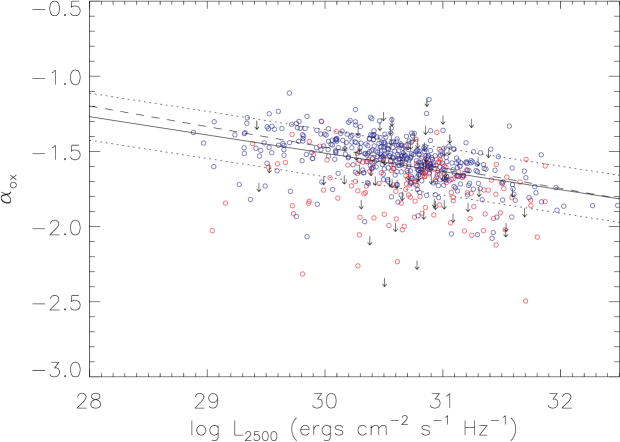
Figure 2 shows the anti-correlation, significant at the 9.0 level ( = -0.20) in the SDSS/XMM Quasar Survey when defined at the conventional 2500 Å and 2 keV fiducial points. The solid line is the best-fit EM regression line for the CENSORED sample:
The slope is consistent within errors to the best-fit regression from Steffen et al. (2006) (dashed line in Fig. 2). Unlike in Steffen et al. (2006), we are not able to reject a correlation between and redshift while controlling for . Instead we find the partial correlation to be marginally significant at the 3.8 level ( = -0.085) in the CENSORED sample. This is likely due to the smaller range in optical luminosity, as well as the large scatter in . Note that in the SPECTRA sample, the partial correlation between and redshift is largely insignificant, except at 1 keV where, again, the scatter is significant (see Table 5).
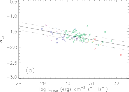
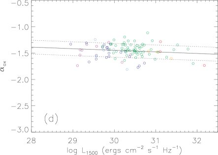
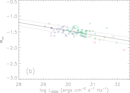
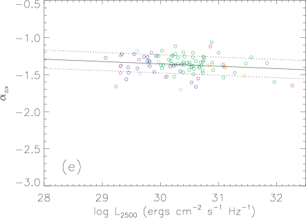
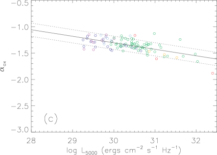
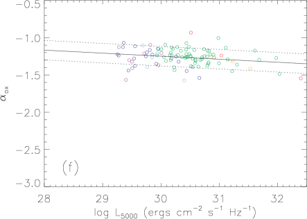
We can now test the correlations of versus optical luminosity using the SPECTRA sample, for each of the six X-ray energies and three optical wavelengths where is defined. Figure 3 shows 6 examples of the relation, defined at 1500, 2500 and 5000 Å and at 1 and 10 keV. The plots show a trend in the slope and dispersion of relation: the slope flattens and the dispersion tightens as the X-ray energy used to define increases. It is clear from the plots that the effect of changing X-ray energy is much stronger than that of changing optical wavelength.
The definition of depends on the baseline over which it is defined; lengthening the baseline can produce an artificial flattening of the slope. To check that the intrinsic slope of the correlation is changing, we define the standard slope by the relation at 2500 Å and 2 keV. We then calculate how the change in baseline affects the slope and intercept of the relation. As the changing baseline frequencies are accompanied by a change in the X-ray flux, we include this effect by assuming an average value for the X-ray slope (). The equations for the change in slope (m) and intercept (b) then become:
and
where is the X-ray frequency at 1, 1.5, 2, 4, 7, or 10 keV and is the optical frequency at 1500, 2500, or 5000 Å.
A change in the optical baseline, for example from 2500 to 5000 Å, affects the slope of the relation by an amount comparable to the error. This is in contrast to Vasudevan et al. (2009), who find a marginal strengthening of the relation as the optical reference point is moved to shorter wavelengths. This may be due to a steepening of the correlation slope, but the small sample size and the strong effect of reddening on the sample do not allow a definitive statement. Since the slope does not depend significantly on optical wavelength in our results, we plot our results only for 2500 Å in Figure 4, in order to focus on the change with X-ray energy.
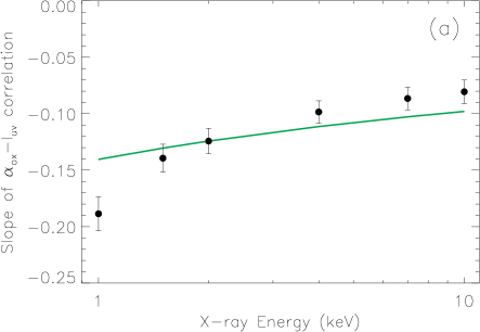
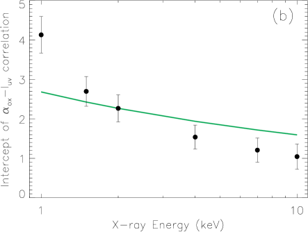
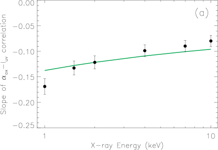
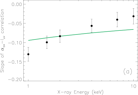
Figure 4 shows that while changing the X-ray baseline clearly has an influence on the measured slopes, the slope for 1 keV is significantly steeper than it would be if the intrinsic correlation were constant. The slopes at 4, 7 and 10 keV are flatter than predicted by the baseline effect at the 1 level. However, since the baseline effect is arbitrarily normalized to the slope at 2 keV, the main result of subtracting the baseline effect is not to assess the significance of the slope at a given energy, but rather to show that the slope of the relation is flattening as X-ray energy increases.
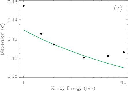
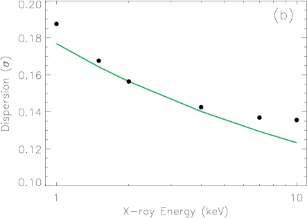
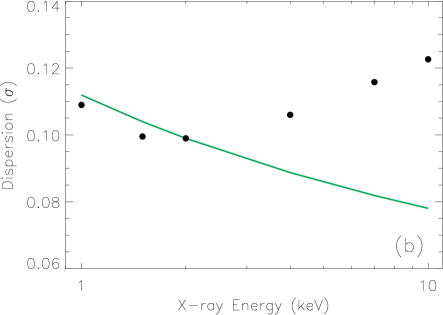
Figure 4 and 4 show the intercept and dispersion of each relation as measured via the least squares fit. The intercept of the relation decreases significantly with X-ray energy compared to the predicted curve. The dispersion of the relation largely follows the predicted curve, though it is larger than predicted at the lowest and highest energies. This is likely due to the larger errors in X-ray flux at the ends of the spectrum.
For low redshift sources, rest-frame energies of 7-10 keV will sample the 7-10 keV observed spectrum, where under- or over-subtraction of the background can alter the measured fluxes and increase the error in the flux measurement. When we exclude sources with z 0.5, we find that the dispersion of the relation at 7 and 10 keV decreases by 0.005, though the dispersions do not decrease all the way to the baseline level. This suggests that the background does have some effect at low redshifts, but it is not the only source of scatter at high energies.
Interestingly, the trend in slope and dispersion of the relation for the CENSORED sample is mostly consistent with the baseline effect (Fig. 5), with a significantly steeper slope than expected at 1 keV. The slopes also show the same marginal flattening at high X-ray energies as the SPECTRA sample. These results are not as strong as in the SPECTRA sample.
Figure 2 suggests that the main effect of including low S/N and undetected sources is an increase in scatter, diluting any potential trends. The red circles in the figure, representing detected sources with no spectral fit, show a weaker anti-correlation, while the blue circles, representing sources with spectral fits, are more strongly anti-correlated. A partial correlation test shows that the correlation decreases in significance from 8.6 ( = -0.284) for sources with S/N 6 to 4.6 ( = -0.131) for sources with S/N 6.
A higher percentage of S/N 6 sources are X-ray weak ( -1.8): 18.7%, compared to only 3.7% in the SPECTRA (S/N 6) sample, where absorbed sources have been excluded. Since absorption cannot be accounted for in the low S/N sources, it is a likely source of the scatter. Figure 6 confirms that though the SPECTRA sample does not remove every X-ray weak source, those with the heaviest optical obscuration (() 0.3) are excluded from the sample. This illustrates the importance of X-ray spectra in excluding absorbed sources.
For the HIGHSNR sample, the slopes show the same trend as found in the SPECTRA sample (cf. Figures 4 and 6), though the errors are larger due to the smaller sample size. Therefore the significant change in slope of the relation is not likely to be due to the effect of undetected absorption in the sources with low S/N X-ray spectra. However, the scatter in the relation defined at low energies does decrease for the HIGHSNR sample (cf. Figures 4 and 6), suggesting that undetected absorption affects the dispersion of the relation when sources with low S/N spectra are included.
Results for the CENSORED, SPECTRA and HIGHSNR samples are summarized in Table 2, which gives the slope, intercept and dispersion for the relation at each X-ray energy for each sample.
4 Discussion
The SPECTRA sample will be used for the following discussion.
4.1 Partial Correlations with Physical Parameters
To gain increased understanding of the trends found above, we tested for correlations with physical parameters. Controlling for the effects of the optical luminosity, we computed the partial correlation coefficient between and black hole mass, Eddington ratio, and redshift.
Black hole masses were derived in Shen et al. (2008) using the width and continuum luminosities of broad emission lines in the optical spectrum: H for 0 z 0.7, MgII for 0.7 1.9, and CIV for 1.9 z 4.5. The broad line region (BLR) is assumed to be virialized, so that the continuum luminosities are related to the BLR radius by the R-L scaling relation, and the emission line widths give the velocities of the BLR clouds. Further details of the line-fitting and scaling relations used for each line can be found in Shen et al. (2008). To calculate the Eddington ratio, we use the Richards et al. (2006) bolometric correction for 3000 Å, = 5.621.14. Though bolometric corrections are by nature uncertain, Figure 12 of Richards et al. (2006) shows that 3000, as well as 5100 Å are regions of relatively small dispersion in the composite SEDs.
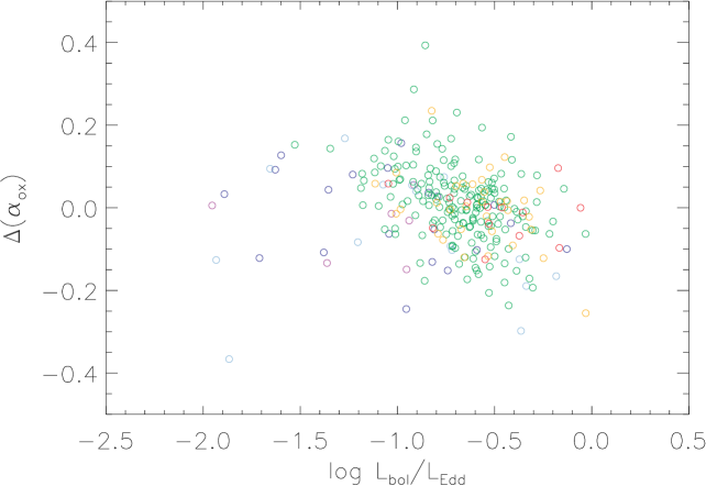
Tables 3-5 list the partial correlation coefficients () and their significance level at each frequency for which is defined. Table 3 compares with black hole mass (MBH), Table 4 compares with the Eddington ratio (Lbol/LEdd), and Table 5 compares with redshift (z). We find that the primary dependence is of on optical luminosity. However, there is a significant partial correlation with Eddington ratio that increases with X-ray energy, with no dependence on optical wavelength (see Fig 8). The strength of the partial correlation suggests that Eddington ratio may play a role in determining .
The partial correlation tests show a marginally significant partial correlation between and redshift (Table 5) but the correlation disappears at higher energies. This is likely due to the large scatter in the relation at 1 keV. The tests show no significant partial correlation between and MBH (Table 3). The black hole masses of the SPECTRA sample range from log MBH = 7.4 to 10 M⊙.
Note that Kelly et al. (2007; see their Fig. 8) found problems with the CENS_TAU program, finding that zero partial correlation between two variables does not necessarily result in a null correlation coefficient (). Assessing the real significance for a given value of the coefficient is therefore difficult at low values. However, given the high value of the partial correlation between and Eddington ratio at high X-ray energies ( 0.3), a significant correlation appears likely.
4.2 Consistency Between , and Lbol/LEdd Relations
In this section, we compare the relation to the relation found in Young et al. (2009). An apparent contradiction arises, as these relations should lead to a secondary relation between and , when in fact the relation is found to be insignificant in the SDSS/XMM-Newton Quasar Survey. This contradiction can be resolved by accounting for the dispersion in the primary relations.
The relation between and (Young et al., 2009) depends on the X-ray energy. The correlation is marginally significant and positive at the lowest energy ( = 0.7 keV) and highly significant and negative at higher energies ( = 4-20 keV). The change in slope of the correlation indicates a pivot in the X-ray spectrum near 1 keV, where the correlation is insignificant.
At 10 keV, the relation is described by
| (1) |
The correlation at 2500 Å and 10 keV is described by
| (2) |
which is equivalent to
| (3) |
Combining equations (1) and (3) should give the following correlation between and :
Such a correlation is not observed to be significant in the SDSS/XMM-Newton Survey (Young et al., 2009; Risaliti et al., 2009), so the relations appear to be inconsistent.
This apparent contradiction can be explained by accounting for the dispersion associated with the Lbol/LEdd relation. The hard (2-10 keV) X-ray slope has been shown to steepen at higher Lbol/LEdd or at larger FWHM(H) (Brandt et al., 1997; Shemmer et al., 2006; Kelly et al., 2007; Risaliti et al., 2009). Shemmer et al. (2008) broke this degeneracy by analyzing a sample of 35 quasars over three orders of magnitude in luminosity, finding a stronger Lbol/LEdd than FWHM(H). A linear fit to the SDSS/XMM-Newton data (Risaliti et al., 2009) gives:
| (4) |
To illustrate the discussion below, a notional SED is shown in Figure 9. The figure shows a simple model of a quasar SED, where specific luminosities are measured at 2500 Å and 1 keV. Since the relation is not significant at 1 keV, using the luminosity at this energy (instead of at 10 keV, as above) allows the focus to be on the effect of the dispersion associated with the Lbol/LEdd relation. In the figure, model (A) illustrates a source with lower (1029 ergs s-1) and model (B) shows a source with higher (1031 ergs s-1). Inserting the optical luminosity into the appropriate relations gives an average value for (dashed lines) and therefore for and .
Since 1 keV is near the pivot point of the X-ray spectrum (Young et al., 2009), the average X-ray slope will not depend on , and so will just be the mean of the sample ( 1.9). The dispersion around the mean will arise from two sources: 1) dispersion associated with the Lbol/LEdd relation (Eqn 4, shown in Figure 9) and 2) dispersion in Lbol/LEdd for a given . While the flattening of the relation with energy implies harder X-ray slope as optical luminosity increases, Fig. 9 shows that this expected hardening is small compared to the dispersion around the mean. Therefore, any secondary relation between would have too large a dispersion for the correlation to be significant.
Moreover, Figure 9 shows how the relation results naturally as a secondary correlation with large scatter. The figure shows that sources at a given lopt with higher hard X-ray luminosities will have harder X-ray slopes, while those with higher soft X-ray luminosities will have softer slopes. The combination of the relation with the -Lbol/LEdd relation thus returns the relations for X-ray energies 1 keV or 1 keV.
4.3 Bolometric Corrections
As can be used to apply a bolometric correction to the hard X-rays (2-10 keV) (e.g., Hopkins et al., 2007) by providing a normalization for the X-ray spectrum, we plot in Figure 10 the dependence of on . Since Lbol is tightly related to the optical luminosity through the bolometric correction, and L2keV is tightly related to L2-10keV through integration over , the linear correlation is expected. However, both the correlation and its dispersion, = 0.12, are of interest when determining X-ray bolometric corrections. For reference, the best-fit line is:
The X-ray weak quasars with very large bolometric corrections ( 1000) do not have enough S/N for X-ray spectral fits. One object is optically red (() = 0.33), so it is possible that these extreme objects are suffering from absorption, affecting both their and values. An additional factor to consider is accretion rate. We find a significant partial correlation between and Lbol/LEdd. The presence of Lbol on both axes can result in a false correlation, but a partial correlation test with Lbol as the third variable shows that the correlation is significant at the 7.7 level, with a = 0.232. The correlation is plotted in Figure 11 with a best fit line:
This correlation is consistent with previous results (e.g., Vasudevan & Fabian, 2009), and suggests that the fraction of disk photons up-scattered to the X-rays decreases as accretion rate increases.
5 Conclusions
We find that the slope of the relation depends on the X-ray energy at which is defined, though there is no significant dependence on optical wavelength. While a change in slope is predicted when the baseline over which is defined increases or decreases, the slopes at the lowest X-ray energy are significantly steeper than predicted, while the slopes at high X-ray energies are marginally flatter than predicted. This suggests that the efficiency of low energy X-ray photon production depends more strongly on the optical/UV photon supply, whereas the efficiency of high energy X-ray photon production remains relatively constant with respect to the seed photon supply. Partial correlation tests show that Eddington ratio is highly correlated with when controlling for , and this partial correlation increases in significance with X-ray energy, suggesting that accretion rate likely plays a role in the results. Nevertheless, remains the primary driver of .
To check the results, we redo the calculations for a sample including low S/N sources (CENSORED) and for a sample including only high S/N sources (HIGHSNR). The CENSORED sample shows the same trends as in the SPECTRA sample, though the results are less significant. This is likely due to the diluting effect of absorption in the low S/N sources, which emphasizes the importance of X-ray spectra in eliminating sources with absorption. The HIGHSNR sample reproduces the trend in the slope of the relation found for the SPECTRA sample, indicating that the results are not affected by undetected absorption. The dispersion of the relation does decrease significantly for the HIGHSNR sample, suggesting that undetected absorption does introduce some error into the determination of X-ray fluxes for sources with moderate S/N.
By combining the relation with the -Lbol/LEdd relation, we can naturally explain two results: 1) the existence of the relation as reported in Young et al. (2009) and 2) the lack of a relation. Given the measured dispersions and correlation coefficients, it is likely that the and - Lbol/LEdd relations are the primary relations, while the relation is secondary. Understanding the relations in this order will give a more complete framework for understanding the relation between optical and X-ray emission in quasars. In order to fully understand the physical implications of the results shown here, a study of the selection, orientation and variability effects is needed. Such a study is now in progress.
Finally, for the purposes of aiding studies of the hard X-ray bolometric correction, we include a description of the - correlation and dispersion. We find a significant partial correlation between and Lbol/LEdd, when taking bolometric luminosity into account as the third variable. This is consistent with a decreasing fraction of up-scattered X-ray photons as accretion rate increases.
References
- Akritas & Siebert (1996) Akritas M.G. & Siebert J. 1996, MNRAS, 278, 919
- Anderson & Margon (1987) Anderson S.F. & Margon B. 1987, ApJ, 314, 111
- Avni, Worrall & Margon (1995) Avni Y., Worrall D.M. & Margon W.A. 1995, ApJ, 454, 673
- Avni & Tananbaum (1982) Avni Y. & Tananbaum H. 1982, ApJ, 262, L17
- Bechtold et al. (2003) Bechtold J. et al. 2003, ApJ, 588, 119
- Beloborodov (1999) Beloborodov A. M. 1999, ApJ, 510, L123
- Bevington et al. (1992) Bevington, P. R. & Robinson, D. K. 1992, Data Reduction and Error Analysis for the Physical Sciences (2d ed; New York: McGraw-Hill)
- Boroson & Green (1992) Boroson, T. A., & Green, R. F. 1992, ApJS, 80, 109
- Brandt et al. (1997) Brandt, W. N., Mathur, S., & Elvis, M. 1997, MNRAS, 285, L25
- Elvis et al. (1994) Elvis M. et al. 1994, ApJ, 95, 1
- Gibson et al. (2009) Gibson et al. 2009, ApJ, 692, 758
- Green & Mathur (1996) Green P. & Mathur S. 1996, ApJ, 462, 637
- Haardt & Maraschi (1991) Haardt F. & Maraschi L. 1991, ApJ, 380, L51
- Hopkins et al. (2007) Hopkins P.F., Richards G.T. & Hernquist L. 2007, ApJ, 654, 731
- Isobe et al. (1986) Isobe T., Feigelson E.D. & Nelson P.I. 1986, ApJ, 306, 490
- Just et al. (2007) Just D.W., Brandt W.N. Shemmer O., Steffen A.T., Schneider D.P., Chartas G. & Garmire G.P. 2007, ApJ, 665, 1004
- Kawaguchi et al. (2001) Kawaguchi T., Shimura T. & Mineshige S. 2001, ApJ, 546, 966
- Kelly et al. (2007) Kelly B.C., Bechtold J., Siemiginowska A., Aldcroft T. & Sobolewska M. 2007, ApJ, 657, 116
- Kelly et al. (2007) Kelly, B. C., Bechtold, J., Trump, J. R., Vestergaard, M., & Siemiginowska, A. 2008, ApJS, 176, 355
- Kriss & Canazares (1985) Kriss G.A. & Canazares C.R. 1985, ApJ, 297, 177
- Lavalley et al. (1992) Lavalley M., Isobe T. & Feigelson E. 1992, ASPC, 25, 245L
- Mainieri et al. (2007) Mainieri et al. 2007, ApJ, 172, 368
- Malkan & Sargent (1982) Malkan M. & Sargent W. 1982, ApJ, 254, 22
- Malzac (2001) Malzac J. 2001, MNRAS, 325, 1625
- Mateos et al. (2005) Mateos et al. 2005, A&A, 433, 855
- Nayakshin (2000) Nayakshin S., Kazanas D. & Kallman T.R. 2000, ApJ, 537, 833
- Pickering et al. (1994) Pickering T.E., Imwanna pipey C.D. & Foltz C.B. 1994, AJ, 108, 5
- Prevot et al. (1984) Prevot M., Lequeux J., Maurice E., Prevot L. & Rocca-Volmerange B. 1984, A&A, 132, 389
- Proga (2007) Proga D. 2007, ApJ,661, 702
- Richards et al. (2003) Richards et al. 2003, AJ, 126, 1131
- Richards et al. (2006) Richards et al. 2006, ApJS, 166, 470
- Risaliti et al. (2009) Risaliti G., Young M. & Elvis M. 2009, astroph/0906.1983
- Shen et al. (2008) Shen Y., Greene J., Strauss M., Richards G. & Schneider D. 2008, ApJ, 680, 169
- Shemmer et al. (2006) Shemmer, O., Brandt, W. N., Netzer, H., Maiolino, R., & Kaspi, S. 2006, ApJ, 646, L29
- Shemmer et al. (2008) Shemmer O., Brandt W.N., Netzer H., Maiolino R. & Kaspi S. 2008, ApJ, 682, 81
- Shields et al. (1978) Shields G.A. 1978, Nature, 272, 706
- Sobolewska et al. (2004a) Sobolewska M.A., Siemiginowska A., Zycki, P.T. 2004, ApJ, 608, 80
- Sobolewska et al. (2004b) Sobolewska M.A., Siemiginowska A., Zycki, P.T. 2004, ApJ, 617, 102
- Spergel et al. (2003) Spergel D.N. et al. 2003, ApJS, 148, 175
- Steffen et al. (2006) Steffen A., Strateva I., Brandt W., Alexander D., Koekemoer A., Lehmer B., Schneider D. & Vignali C. 2006, AJ, 131, 2826
- Strateva et al. (2005) Strateva I.V., Brandt W.N., Schneider D.P., Vanden Berk D.G. & Vignali C. 2005, ApJ, 130, 387
- Tananbaum et al. (1986) Tananbaum H., Avni Y., Green R.F., Schmidt M. & Zamorani G. 1986, ApJ, 305, 57
- Tang et al. (2007) Tang S.M., Zhang S.N. & Hopkins P. 2007, MNRAS, 377, 1113
- Vanden Berk et al. (2001) Vanden Berk D.E. et al. 2001, AJ, 122, 549
- Vasudevan & Fabian (2009) Vasudevan, R.V. & Fabian A.C. 2009, MNRAS, 392, 1124
- Vasudevan et al. (2009) Vasudevan, R.V., Mushotzky R.F., Winter L.M., & Fabian A.C. 2009, MNRAS, 399, 1553
- Vignali et al. (2003) Vignali C., Brandt W.N. & Schneider D.P. 2002, AJ, 125, 443
- Ward et al. (1987) Ward M.J., Elvis M., Fabbiano G., Carleton N.P., Willner S.P. & Lawrence A. 1987, ApJ, 315, 74
- Wilkes et al. (1994) Wilkes B.J., Tananbaum H., Worrall D.M., Avni Y., Oey M.S. & Flanagan J. 1994, ApJS, 92, 52
- Wills, Netzer & Wills (1985) Wills B.J., Netzer H. & Wills D. 1985, /apj, 288, 94
- Young et al. (2009) Young M., Elvis M. & Risaliti G. 2009, ApJS, 183, 17
- Yuan et al. (1998) Yuan W., Siebert J. & Brinkmann, W. 1998, AA, 394, 498
- Zdziarski et al. (1999) Zdziarski A. A., Lubinski, P., & Smith, D. A. 1999, MNRAS, 303, L11
- Zdziarski et al. (2000) Zdziarski A. A., Poutanen J. & Johnson W.N. 2000, ApJ, 542, 703
| Sample name | Ntot | S/N | median NH | z | mag | % targets |
|---|---|---|---|---|---|---|
| CENSORED | 514 | all | 0.39 | 0.1-5.0 | 15.2-20.7 | 2% |
| SPECTRA | 327 | S/N 6 | 0.39 | 0.1-4.4 | 15.2-20.4 | 3% |
| HIGHSNR | 99 | S/N 20 | 0.06 | 0.1-3.0 | 15.6-19.9 | 9% |
Note. — All three samples exclude RL and BAL quasars, sources with significant intrinsic absorption, and sources with bad fits to the X-ray spectrum.
| X-ray Energy | CENSORED | SPECTRA | HIGHSNR | ||||||
|---|---|---|---|---|---|---|---|---|---|
| Slope | Intercept | Slope | Intercept | Slope | Intercept | ||||
| 1 keV | -0.170.02 | 3.470.47 | 0.19 | -0.190.02 | 4.130.46 | 0.15 | -0.130.02 | 2.450.54 | 0.11 |
| 1.5 keV | -0.130.01 | 2.430.42 | 0.17 | -0.140.01 | 2.700.38 | 0.13 | -0.100.02 | 1.550.50 | 0.10 |
| 2 keV | -0.120.01 | 2.130.39 | 0.16 | -0.120.01 | 2.270.35 | 0.11 | -0.08.02 | 1.090.49 | 0.10 |
| 4 keV | -0.0990.01 | 1.490.35 | 0.14 | -0.0980.01 | 1.540.30 | 0.10 | -0.060.02 | 0.300.53 | 0.11 |
| 7 keV | -0.0900.01 | 1.260.34 | 0.14 | -0.0860.01 | 1.210.31 | 0.10 | -0.040.02 | -0.150.58 | 0.12 |
| 10 keV | -0.0800.01 | 0.970.34 | 0.13 | -0.0810.01 | 1.040.32 | 0.11 | -0.030.02 | -0.400.61 | 0.12 |
Note. — Slopes, intercepts, and dispersions for each of the three samples at each X-ray energy, using 2500 Å as the optical wavelength. Errors are at the 1 level.
| X-ray Energy (keV) | 1500 Å | 2500 Å | 5000 Å |
|---|---|---|---|
| 1.0 | -0.070 (1.84) | -0.064 (1.68) | -0.065 (1.71) |
| 1.5 | -0.036 (0.97) | -0.030 (0.81) | -0.032 (0.86) |
| 2.0 | -0.013 (0.35) | -0.0071 (0.20) | -0.0093 (0.26) |
| 4.0 | 0.048 (1.37) | 0.053 (1.51) | 0.047 (1.38) |
| 7.0 | 0.093 (2.66) | 0.096 (2.82) | 0.086 (2.53) |
| 10.0 | 0.11 (3.14) | 0.10 (2.94) | 0.10 (2.94) |
Note. — The partial correlation coefficient listed is Kendall’s , with its significance () in parantheses. Correlations with significance above 3.3 (P 99.9%) are considered to be significant. These are the results for the SPECTRA sample.
| X-ray Energy (keV) | 1500 Å | 2500 Å | 5000 Å |
|---|---|---|---|
| 1.0 | -0.13 (3.25) | -0.12 (3.00) | -0.12 (3.00) |
| 1.5 | -0.17 (4.25) | -0.16 (4.00) | -0.16 (4.00) |
| 2.0 | -0.19 (4.87) | -0.19 (4.87) | -0.19 (4.87) |
| 4.0 | -0.27 (7.11) | -0.27 (7.11) | -0.27 (7.11) |
| 7.0 | -0.32 (8.21) | -0.32 (8.21) | -0.32 (8.21) |
| 10.0 | -0.33 (8.25) | -0.33 (8.25) | -0.33 (8.25) |
Note. — The partial correlation coefficient listed is Kendall’s , with its significance () in parantheses. Correlations with significance above 3.3 (P 99.9%) are considered to be significant. These are the results for the SPECTRA sample.
| X-ray Energy (keV) | 1500 Å | 2500 Å | 5000 Å |
|---|---|---|---|
| 1.0 | -0.16 (4.32) | -0.15 (4.05) | -0.14 (0.036) |
| 1.5 | -0.11 (3.14) | -0.097 (2.77) | -0.087 (2.56) |
| 2.0 | -0.090 (2.65) | -0.074 (2.18) | -0.064 (1.88) |
| 4.0 | -0.040 (1.21) | -0.027 (0.84) | -0.021 (0.66) |
| 7.0 | -0.022 (0.67) | -0.011 (0.33) | -0.010 (0.31) |
| 10.0 | -0.015 (0.45) | -0.013 (0.41) | 0.0086 (0.26) |
Note. — The partial correlation coefficient listed is Kendall’s , with its significance () in parantheses. Correlations with significance above 3.3 (P 99.9%) are considered to be significant. These are the results for the SPECTRA sample.