SLAC-PUB-13759 Strange Bedfellows: Quantum Mechanics and Data Mining

Abstract

Last year, in 2008, I gave a talk titled Quantum Calisthenics. This year I am going to tell you about how the work I described then has spun off into a most unlikely direction. What I am going to talk about is how one maps the problem of finding clusters in a given data set into a problem in quantum mechanics. I will then use the tricks I described to let quantum evolution lets the clusters come together on their own.

1 What Is This About ?

Since I am talking to you at Light Cone 2009, it is fun for me to point out that a good deal of the material I will present is a direct spin-off of material I presented last year in my talk, Quantum Calisthenics. What is new (and surprising to me) is that the ideas for solving problems in quantum mechanics would prove extremely useful in dealing with data-mining, a problem in computer science that, at first glance, does not appear to have anything to do with quantum physics, or for that matter, with any kind of physics. In the next few minutes hope to convince you that despite appearances data-mining and quantum physics are a match made in heaven.

1.1 What Is The Problem And How Does It Affect You ?

As one wag said, the problem of data-mining can be summarized by, ”If a supermarket customer buys formula and diapers, how likely are they to buy beer?”. Clearly, if it is possible to give a good answer to this question, a supermarket manager can decide if it is better to put the beer next to the diapers, or to put it at the other end of the store to encourage impulse buying.

As amusing as this simple summary may be, there is a bit more to the story. For example, other businesses that engage in data-mining are Amazon and NETFLIX. Both companies have large data bases containing the information about each customer’s previous purchases. Their goal in mining this data is to suggest what the next book a given customer might like to purchase, or movie she might like to rent. They base their suggestion on what they believe customers like her have purchased or rented. The key question is how do they determine who is a customer like her ? In general the examination of unstructured data to find clusters that are similar in some way is a key element of data-mining. The search for these structures in a data-set is imaginatively referred to as clustering.

While the use of clustering by Amazon and NETFLIX may improve the shopping experience, data-mining affects all of us in ways that impact out existence at a much more important level. This happens when banks and insurance companies apply it to the problem of scoring. Basically, the idea is to take all of the data they have about people and identify clusters of similar people so as to predict how likely it is that an applicant will default on a mortgage, or loan, or how likely they are to be robbed, die, etc.. To do this they take their and try, in various ways, to find clusters of people that they can define as similar. For better or worse we are all affected by these practices.

Finally, to give one of a myriad of examples that have nothing to do with questions of business, let us consider the case of gene chips as a tool for medical diagnosis and treatment planning. Gene chips are a technology for measuring which genes are being under or over-expressed by a cell. The idea is that understanding the different patterns of gene expression and how they relate to specific diseases and drug resistance will allow a doctor to both diagnose a disease and prescribe the correct drug for treating it. Later I will talk about a specific example of this sort of study for the case of patients with Type A or Type B Leukemia.

Summarizing we can say that many fields - physics, biology, medicine intelligence and homeland security, finance, insurance, and diplomacy - all collect large databases of information. Sorting through such data and searching for previously unknown interesting and relevant structures is referred to as data-mining. Clearly from the breadth of topics one might guess that no precise definition of data-mining exists. However, although we can’t make the definition of what we wish to do totally specific, it is intuitively clear that it is a useful notion. In what follows I will be describing a clustering technique that my colleague David Horn and I call DQC (Dynamic Quantum Clustering). I hope that the specific examples that I discuss will give you a flavor for the general problem. A more complete exposition of this material is given in Ref.[1].

2 The Data Miner’s Lament: The Curse of High Dimension

The general problem is we are given a database with a large number of entries. Associated with each entry is a record that contains all of the information that has been collected about that entry, each such item of information is called a feature. Clearly the number of features and the type of information stored in each feature varies from database to database. As an example, let’s talk about NETFLIX. Assume that they have a library of 10,000 films that can be rented. Then each entry in the database might correspond to a customer and associated to each customer would be 10,000 features (in numerical format) that indicate which films the customer has rented and, if available, his/her rating of each of those films. The number of features is called the dimension of the problem. Thus, we see that finding clusters of people with similar tastes in the NETFLIX problem involves searching for clusters in a space of very high dimension. It should not surprise you that this is computationally difficult.

Because it is so difficult to search for clusters in spaces of high dimension, people try to find a way to reduce the dimension of the problem without, too badly, compromising the information. The tool most commonly used to accomplish this is SVD or Singular Value Decomposition. Clearly, given the time available to me I can’t go into the use of SVD too deeply, but I would like to take a few moments to give you a feeling for what it does and doesn’t do.

2.1 Singular Value Decomposition: The Swiss Army Knife of Data Mining

SVD, or Singular Value Decomposition, is the statement that any $n\times m$-matrix can be brought to an almost diagonal form. The first time I was introduced to this theorem many years ago I couldn’t believe it was really good for anything. That just goes to show what I knew. In fact, nowadays, SVD has crept into all sorts of areas of physics and data-mining. It is extensively used in solid state physics computations based on the DMRG (or density matrix renormalization group) method, in image compression, in data-mining to do - among other things - dimensional reduction, and a host of other places. There is much I could say to try and expose you to its many applications, but time being what it is I will limit myself to giving a brief introduction to the SVD decomposition and an example of how we will use it.

Basically SVD is useful to us because all of the data we will mine will be presented in the form of an $n\times m$-matrix of numerical values. Each row of this matrix will correspond to the entries in the data base (i.e., customers, events in a physics experiment, the specific cell culture corresponding to a given gene-chip map, etc.). The columns of the matrix represent the features that have been measured for each entry in the database. The theorem establishing the SVD decomposition says that for any $n\times m$-matrix $M$, there exists a unitary $n\times n$-matrix $U$, an $n\times m$-matrix $S$ and a unitary $m\times m$-matrix $V$, such that

$$M=U\,S\,V^{\dagger}.$$ (1)

where the matrix $S$ only has non-vanishing entries along the diagonal. Consider the explicit example:

$$\left(\begin{array}[]{cc}\hskip-2.0pt\hskip-2.0pt8.3\hskip-2.0pt&\hskip-2.0pt5.8\hskip-2.0pt\hskip-2.0pt\\ \hskip-2.0pt\hskip-2.0pt-4.5\hskip-2.0pt&\hskip-2.0pt-4.3\hskip-2.0pt\hskip-2.0pt\\ \hskip-2.0pt\hskip-2.0pt6.8\hskip-2.0pt&\hskip-2.0pt-8.5\hskip-2.0pt\hskip-2.0pt\\ \end{array}\right)\hskip-2.0pt\hskip-2.0pt\hskip-2.0pt\hskip-2.0pt = \hskip-2.0pt\hskip-2.0pt\hskip-2.0pt\hskip-2.0pt\left(\begin{array}[]{ccc}\hskip-2.0pt-0.85\hskip-2.0pt&\hskip-2.0pt0.077\hskip-2.0pt&\hskip-2.0pt-0.522\hskip-2.0pt\hskip-2.0pt\\ \hskip-2.0pt\hskip-2.0pt0.51\hskip-2.0pt&\hskip-2.0pt-0.133\hskip-2.0pt&\hskip-2.0pt-0.85\hskip-2.0pt\hskip-2.0pt\\ \hskip-2.0pt\hskip-2.0pt-0.135\hskip-2.0pt&\hskip-2.0pt-0.988\hskip-2.0pt&\hskip-2.0pt0.074\hskip-2.0pt\hskip-2.0pt\\ \end{array}\right)\cdot\hfill$$ (14)

$$\hskip-15.0pt\left(\begin{array}[]{cc}\hskip-2.0pt\hskip-2.0pt11.875\hskip-2.0pt&\hskip-2.0pt0\hskip-2.0pt\hskip-2.0pt\\ \hskip-2.0pt\hskip-2.0pt0\hskip-2.0pt&\hskip-2.0pt10.907\hskip-2.0pt\hskip-2.0pt\\ \hskip-2.0pt\hskip-2.0pt0\hskip-2.0pt&\hskip-2.0pt0\hskip-2.0pt\hskip-2.0pt\\ \end{array}\right)\cdot\left(\begin{array}[]{cc}\hskip-2.0pt\hskip-2.0pt-0.864\hskip-2.0pt&\hskip-2.0pt-0.503\hskip-2.0pt\hskip-2.0pt\\ \hskip-2.0pt\hskip-2.0pt-0.503\hskip-2.0pt&\hskip-2.0pt0.864\hskip-2.0pt\hskip-2.0pt\\ \end{array}\right),$$

where $M$ is the matrix on the left hand side of the equation and $U$, $S$ and $V^{\dagger}$ are the three matrices on the right hand side of the equation.

Now, to get a feeling for what is decomposition is doing for us, let us think of the rows of $M$ as the coordinates of three different points in two dimensions. Clearly these three vectors cannot all be linearly independent as there can only be two linearly independent vectors in $2$-d. The SVD decomposition gives us a coordinate system for plotting these points that is adapted to the way the data is spread out. To be more specific we note that the two rows of $V^{\dagger}$ are two ortho-normal vectors that span the space containing the points. From the formula for $M$ we see that each of the original points can be written as linear combination of the two rows of $V^{{\dagger}}$. The coefficient of each of these two basis vectors is given by the entries in the first two rows of $U$ times the corresponding elements of $S$. From this we see that the rows of $U$ serve as coordinates for each of the data points, where the data has been mapped onto the unit sphere (since each row of $U$ is a unit vector). If one wishes to dimensionally reduce the clustering problem one can use a smaller number of columns of the $U$-matrix to label the points. In this case we typically rescale each row to have unit length. In all of the examples that follow we have done this step before starting the DQC procedure.

Another use of SVD is to reduce the amount of data used to describe a picture as either a way of filtering out noise, or as a first step towards image recognition. To see how this works assume that a picture is given by a matrix, $M$, of pixels. Another way to write the SVD decomposition of this matrix is

$$M_{ij}=\sum_{\nu=1}^{N_{max}}S_{\nu\nu}\,t^{\nu}_{i,j}$$ (15)

where the numbers $\lambda_{\nu}$ run over the non-zero numbers on the diagonal of $S$ (in decreasing order) up to a maximum, $N_{max}$, and the matrices $t^{\nu}_{ij}$ are given by

$$t^{\nu}_{i,j}=U_{i\nu}\,V^{{\dagger}}_{\nu j}.$$ (16)

This is a useful way of looking at things because the diagonal entries in $S$ tend to decrease rapidly. Thus, since $U$ and $V^{{\dagger}}$ (and thus $V$) are unitary matrices, we see that

$$\sum_{i,j}M^{2}_{ij}=\sum_{\nu}S_{\nu\nu}^{2}.$$ (17)

If we approximate the original picture by a sum over the $N$ largest entries in $S$; i.e.,

$$M^{approx}_{ij}=\sum_{\nu=1}^{N}S_{\nu\nu}\,t^{\nu}_{ij}$$ (18)

then it follows that

$$\sum_{i,j}(M-M^{approx})^{2}_{ij}=\sum_{\nu=N+1}^{N_{m}ax}S_{\nu\nu}^{2}$$ (19)

and so, we see that the sum of the squares of all of the errors in the pixels is bounded by the sum of the square of the eigenvalues $S_{\nu\nu}$ that weren’t included in the approximation.

2.2 What About Clustering ?

To this point I have only been talking about using the SVD decomposition to plot the data in a coordinate system that is adapted to the natural structure of the data. Thus the first axis is the one in which the data had the largest variance; i.e. had the biggest difference between the largest and smallest coordinate values, the second axis is the direction in which the data has the next largest variance, and so on. While this step is useful and dimensionally reducing the data by keeping only the coordinates corresponding to the first few directions can lead to plots that in some loose sense maximally separate data belonging to different clusters, in general this is only a first step.

In the generic situation, especially for data that cannot usefully be reduced to two or three dimensions, clusters cannot be easily identified. The situation is even more complicated if the data does not group into separated globular clusters, but instead is concentrated on some other geometrical structure, say for example, a ring. In this case SVD followed by strong dimensional reduction can incorrectly lead one to conclude there are clusters where none exist. This is where DQC comes into play. DQC allows one to explore more dimensions of the original data and it can clearly indicate the presence of higher dimensional geometries when they exist.

3 DQC: What Is Dynamic Quantum Clustering?

In Dynamic Quantum Clustering, DQC, we map the problem of finding clusters into a problem in quantum mechanics and then use the techniques of quantum mechanics to allow the clusters, or over dense regions in the data, to reveal themselves.

3.1 The Parzen Window Estimator

An old approach in clustering was the so-called Parzen Window Estimator. The crux of this idea was that given $n$-dimensional data, denoted by points $\vec{x_{i}}$, one could construct a function on the $n$-dimensional Euclidean space as follows:

$$\psi(\vec{x})=\sum_{i}e^{-{1\over 2\sigma^{2}}(\vec{x}-\vec{x_{i}})\cdot(\vec{x}-\vec{x}_{i})}$$ (20)

In other words, the Parzen estimator is simply a sum of $n$-dimensional Gaussians with a common width determined by the parameter $\sigma$. The notion was that in regions where the data was denser, the Parzen estimator would have a relative maximum. The hope was that clusters could be identified by finding these maxima and selecting a region about each one, so that the points in that region would be said to belong to a cluster. There were several problems with the Parzen estimator approach. First, finding the maxima of a complicated function in an $n$-dimensional space is computationally time consuming. Second, the structure of the function proved to depend sensitively on the choice of $\sigma$. For a value of $\sigma$ that is too small, one obtains a function with many local maxima and very small clusters. If $\sigma$ is to large the maxima all coalesce and no distinct clusters can be found.

3.2 Quantum Clustering

Quantum clustering, (QC), begins with the construction of a Parzen estimator20, but instead of using the Parzen estimator to find clusters directly, we use it to construct a potential function whose minima are related to the clusters. The construction of this function was first introduced in the paper of Horn and Gottlieb[2] where it was defined by the condition that it is the function $V(\vec{x})$ for which the Parzen estimator satisfies the $n$-dimensional time-independent Schrödinger  equation

$$H\psi=\left(-{\sigma^{2}\over 2}\vec{\nabla}^{2}+V({\vec{x}})\right)\psi=0.$$ (21)

That such a $V(\vec{x})$ always exists is clear, all one has to do is to solve equation 21 for $V(\vec{x})$; i.e.,

$$V(\vec{x})=-{\sigma^{2}\over 2\,\psi(\vec{x})}\,\vec{\nabla}^{2}\,\psi(\vec{x}).$$ (22)

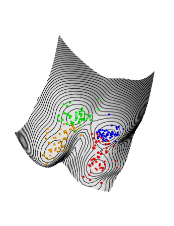
The intuition behind this prescription is based upon the fact that in the quantum problem local maxima in the ground state wave-function correspond to local minima in the potential; moreover, such minima are likely to be a good deal sharper and deeper than the corresponding maxima of the wave-function, due to the fact that the kinetic term, $-\vec{\nabla}^{2}$, causes the wave-function to be more spread out than the features of the potential would suggest. A sample of such a potential function will be shown in the next section when I discuss the example of Ripley’s Crab Data.

In the orginal quantum clustering approach[2] points lying in the basin of attraction of particular minimum were identified as a single cluster. One way of determining which minimum was closest to a given point was to classically roll the points downhill using the gradient descent method. The disadvantages to this method are: first, it can be computationally very expensive to carry out when there a large number of points and a large number of features involved; second, there can be many instances where a slightly too small value for $\sigma$ can lead to a potential with several nearby shallow minima contained in a single larger minimum. When this happens the classical prescription will lead to several small clusters and not show the existence of the larger cluster. As we will see, by appropriately choosing one of the two parameters that control the DQC evolution, this sensitivity upon the choice of $\sigma$ can be greatly reduced and the structure of such nearby minima can be explored even in problems with a large number of features.

3.3 Ripley’s Crab Data

As a simple example of the construction of the potential associated with a data set let us consider the data on the morphology of rock crabs that was used in the book on Pattern Recognition and Neural Networks by R.D.Ripley[3]. The problem in this exercise is to see how well one can classify the members of a collection of 200 crabs; the collection contains 100 crabs of two different species and each set of 100 is further subdivided into 50 crabs of each sex. The only information one has consists of five measurements of carapace size and claw size. In the picture I have shown I have plotted a potential in two-dimensions. The colored dots correspond to real classes. To construct this potential we did an SVD decomposition of the data-matrix and then used the second and third principal component to construct the potential. As you can see from the picture the potential has four local minima and, except for a few outliers, the different species and sexes are identified by the valley in which they lie.

Figure 1: This is a plot of the quantum potential function for the two-dimensional problem of the Ripley’s Crab Data where the coordinates of the data points are chosen to be given by the second and third principal components. The four known classes of data points are shown in different colors and are placed upon the potential surface at their original locations.

3.4 DQC: Dynamic Quantum Clustering

DQC begins by constructing the same potential function used in quantum clustering, it differs in how one handles the problem of how to identify data points with local minima of the function in $N$-dimensions. We simply exploit the fact that from the outset we are dealing with a quantum problem and a well defined Hamiltonian. To roll the different data points down hill we simply evolve each Gaussian wave-function using the time development operator

$$U(t)=e^{-i\,H\,t},$$ (23)

so that the evolution of any state $\psi_{i}(\vec{x})$ is defined to be

$$\psi(\vec{x},t)=e^{-i\,H\,t}\,\psi(\vec{x}).$$ (24)

This time evolved state is the solution to the time-dependent Schrödinger  equation

$$i{\partial\psi_{i}(\vec{x},t)\over\partial t} = H\psi_{i}(\vec{x},t)$$ (25)

$$= \left(-{\nabla^{2}\over 2m}+V(\vec{x})\right)\psi_{i}(\vec{x},t),$$

The important feature of quantum dynamics, which makes the evolution so useful in the clustering problem, is that according to Ehrenfest’s theorem, the time-dependent expectation value

$$\langle\psi(t)|\,\mbox{$\vec{x}$}\,|\psi(t)\rangle=\int\,d\mbox{$\vec{x}$}\,\psi^{\ast}_{i}(\vec{x},t)\,\mbox{$\vec{x}$}\,\psi_{i}(\vec{x},t),$$ (26)

satisfies the equation,

$${d^{2}\langle\,\vec{x}(t)\rangle\over dt^{2}} = -{1\over m}\int d\vec{x}\psi^{\ast}_{i}(\vec{x},t)\,\vec{\nabla}V(\vec{x})\,\psi_{i}(\vec{x},t)$$ (27)

$$= -{1\over m}\,\langle\psi(t)|\,\vec{\nabla}V(\vec{x})\,|\psi(t)\rangle.$$ (28)

If $\psi_{i}(\mbox{$\vec{x}$})$ is a narrow Gaussian, this is equivalent to saying that the center of each wave-function rolls towards the nearest minimum of the potential according to the classical Newton’s law of motion. This means we can explore the relation of this data point to the minima of $V(\vec{x})$ by following the time-dependent trajectory $\langle\,\vec{x}_{i}(t)\,\rangle=\langle\psi_{i}(t)|\,\vec{x}\,|\psi_{i}(t)\rangle$. Clearly, given Ehrenfest’s theorem, we expect to see any points located in, or near, the same local minimum of $V(\vec{x})$ to oscillate about that minimum, coming together and moving apart. In our numerical solutions we generate animations which display this dynamics for a finite time. This allows us to visually trace the clustering of points associated with each one of the potential minima.

At first glance this approach would seem to be a step backwards since we have replace solving ordinary classical differential equations by the problem of solving more complicated partial differential equations, but this is incorrect. The trick is to think of the problem reduced to the subspace of the full Hilbert space spanned by the original data points. While this is not completely equivalent to the original problem, for our purposes the accuracy of the approximation is good enough to capture the same clusters.

Clearly, these states are not orthogonal to one another, however we can choose an orthonormal set of states that span the subspace by computing the matrix

$$N_{ij}=\langle\psi_{i}(\vec{x})|\psi_{j}(\vec{x})\rangle$$ (29)

and then computing its eigenvectors. The eigenvectors corresponding to non-vanishing eigenvalues form a set of orthogonal linear combinations of the original states and they are normalized by dividing each eigenstate by the inverse square root of its eigenvalue. The fact that the initial states are all Gaussians makes computing $N_{ij}$ analytically a trivial exercise. Furthermore, the Gaussian nature of the original states also makes it simple to calculate the matrix elements of the Hamiltonian and the position operators $X_{k}$ (these operators act on our wavefunctions by multiplying them by the $x_{k}$ coordinate).

$$H_{ij}=\langle\psi_{i}(\vec{x})|\,H\,|\psi_{j}(\vec{x})\rangle,$$ (30)

where $H$ is defined to be

$$H = {\vec{p}^{2}\over 2\,m}+V(\vec{x})$$ (31)

$$= -{\vec{\nabla}^{2}\over 2\,m}+V(\vec{x}).$$

and

$$X_{ij}=\langle\psi_{i}(\vec{x})|\,X_{k}\,|\psi_{j}(\vec{x})\rangle.$$ (32)

(Note: I have introduced the parameter $m$ into the Hamiltonian used to evolve the states. This is different from the $\sigma$ used to construct the potential. I do this so that by choosing $m<1$ I can increase the effect of quantum tunneling and decrease the sensitivity by causing points in nearby minima to merge.)

Given the analytical expressions for these matrix elements between the Gaussian states it is a simple matter to compute the same operators in the orthonormal basis defined by $N_{ij}$ and to then exponentiate the Hamiltonian in this basis. In this way the apparently difficult problem of solving the time-dependent Schrödinger  equation is reduced to the computation of simple closed form expressions followed by numerical evolution in the truncated Hilbert space. This trick reduces the problem to dealing with matrices whose size is determined by the number of data points and not the dimension of the data-set (i.e., the number of features associated with each data point). Of course, when there are a large number of data-points this might seem to be an intractable problem however, fortunately, there is a simple trick for dealing with that situation too.

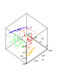
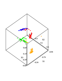
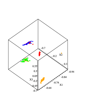
Applying these ideas to Ripley’s crab data, reduced to the first three principle components, is very instructive. (The evolution of the full five-dimensional data-set shows exactly the same behavior but is more complicated to plot.) In the following pictures I show two steps in the time evolution of the initial distribution. The first picture is a snapshot of the original data before evolution has begun. In the next picture we see what happens after a short time. As expected the points begin to approach one another. The last picture shows what happens if we stop the points where they are and restart DQC using the new points. The clustering is quite easy to see and it is easy to understand why the data is clustering as it is.

  

Figure 2: The left hand plot shows three-dimensional distribution of the original data points before quantum evolution. The middle plot shows the same distribution after quantum evolution. The right hand plot shows the results of an additional iteration of DQC. The values of parameters used to construct the Hamiltonian and evolution operator are: $\sigma=0.07$ and $m=0.2$. Colors indicate the expert classification of data into four classes, unknown to the clustering algorithm. Note, small modifications of the parameters lead to the same results.

4 Exploiting DQC

Obviously, in this brief overview of DQC, I have not given you all the details of how to implement the algorithm, but I have given you all of the essentials. Now I want to point out that although colors in Fig.2 were there so that you could see the clusters form and tell how well DQC was working, the fact that colors can be used in the visualization step can play an additional role in data mining. The crab problem was an example of a blind search for clusters. What I want to concentrate on now is a different sort of problem; namely, a situation where we start with a classification of the data into clusters, but we do not know how the measured features in the data-set relate to the classification. As an example, consider Affymetrix gene chip data for a set of Leukemia patients. The Affymetrix gene chip is a silicon device to which strands of RNA are attached in a regular matrix. The setup is made so that, if a protein binds to a strand of RNA that codes for that protein the the spot to which the strand is bound flouresces when light shines on the chip. Such a gene chip can measure the expression of over 7000 genes (by seeing the proteins that are coded for by that gene). Now, in the case of ALL and AML leukemia cells we start with a clinical classification based upon a pathological examination of the cells. So we know how to color spots in the DQC picture according to type. What we don’t know is how to use the gene chip information to identify these cells; that is what we want to do using DQC (or any other clustering method). Two problems that one has, in addition to the clustering problem, is that the binding of a protein to a strand of RNA is not all that specific, and most of the genes being measured have nothing to do with cancer. That is where the coloring comes in. If one applies DQC to such a data set and sees clusters of the correct color form, then one knows that the gene chip data contains the information we need. The next step is to eliminate features (i.e., measurements of particular genes) without hurting the clustering. (There are various schemes for doing this, including the brute force approach.) Clearly, if we pursue this process and weed out genes that have nothing to do with the clustering, then one goes a long way to both developing a diagnostic tool, and obtaining an insight into which genes are related to the specific cancer.

I will show you some results for a data set by Golub et.al.[4]. This set contains gene chip measurements on cells from 72 leukemia patients with two different types of Leukemia, ALL and AML. The expert identification of the classes in this data set is based upon dividing the ALL set into two subsets corresponding to T-cell and B-cell Leukemia. The AML set is divided into patients who underwent treatment and those who did not. In total the Affymetrix GeneChip used in this experiment measured the expression of 7129 genes. The specific feature filtering method we employed in this analysis was based on SVD-entropy, and is a simple modification of a method introduced by Varshavsky et al.[5] and applied to the same data. For our purposes it doesn’t matter what the feature filtering method was, I want you to see the difference removing features makes in clustering. I also want you to recognize how the DQC visualization makes it easy to quickly identify the effect of removing features from the data.

 

Figure 3: The left hand picture is the raw data from the Affymetrix Chip plotted for principal components 2,3,4. Clearly, without the coloring it would be hard to identify clusters. The right hand picture is the same data after DQC evolution using $\sigma=0.2$ and a mass $m=0.01$. The different classes are shown as blue, red, green and orange.

 

Figure 4: The left hand plot is the Golub data after one stage of SVD-entropy based filtering, but before DQC evolution. The right hand plot is the same data after DQC evolution.

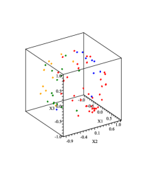
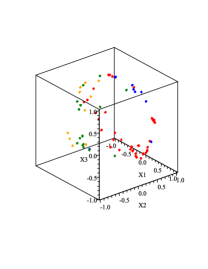
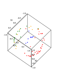
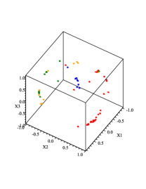
Figure 3 displays the raw data in the 3-dimensional space defined by the second to fourth principal components, and the effect that DQC has on these data. In Figure 4 we see the result of applying feature filtering to the original data, represented in the same 3-dimensions, followed by DQC evolution. Applying a single stage of filtering has a dramatic effect upon clustering, even before DQC evolution. The latter helps sharpening the cluster separation.

 

Figure 5: The left hand plot is the data after three stages of SVD-entropy based filtering, but before DQC evolution. The right hand plot is the same data after DQC evolution.

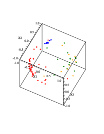
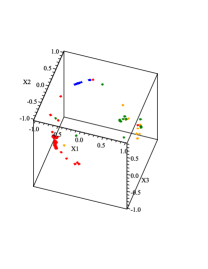
Figure 5 shows the results of removing many features (using the SVD entropy method) before and after DQC evolution. These plots, especially the after DQC pictures, show dramatic clustering, especially for the blue points. With each stage of filtering we see that the blue points cluster better and better, in that the single red outlier separates from the cluster and the cluster separates more and more from the other points. The blue points are what I refer to as an obviously robust cluster identified in early stages of feature filtering. If one continues removing features, however, the clear separation of the blue points from the others begins to diminish. This tells us that we have gone to far with the blue points, we are now removing features that matter for its classification. This is, of course, just what we are looking for, a way of identifying those features which are important to the existing biological clustering. We could, at this juncture, search among the most recent 278 eliminated features to isolate those most responsible for the separation of the blue cluster from the others. Now however I want to make another point. Since the blue cluster is so robust and easily identified, let us remove the blue cluster from the original data and repeat the same process without this cluster. The idea here is that now the SVD-entropy based filtering will not be pulled by the blue cluster and so it will do a better job of sorting out the red, green and orange clusters. I want you to see that this is in fact the case.

 

Figure 6: The left hand plot is what the starting data looks like if one first removes the blue points and does one stage of SVD-entropy based filtering. The right hand plot is what the starting data looks like after three stages of filtering.

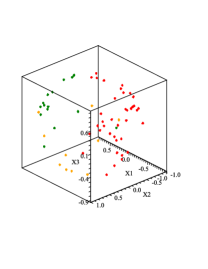
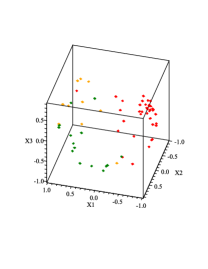
In Figure 6 we see a plot of what the starting configurations look like if one takes the original data, removes the blue cluster and re-sorts the reduced data set according to the SVD-entropy based filtering rules. The left hand plot is what happens if one filters a single time. The right hand plot shows what happens if one repeats the filtering procedure two more times, It is clear from the plots that each iteration of the filtering step improves the separation of the starting clusters. By the time we have done five filtering steps the red, green and orange clusters are distinct, if not obviously separated.

 

Figure 7: The left hand plot is what the starting data looks like if one first removes the blue points and does five stages of SVD-entropy based filtering. The right hand plot is what happens after one stage of DQC evolution. The bottom plot is the final result after iterating the DQC evolution step two more times. At this point the clusters are trivially extracted.

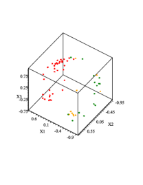
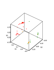
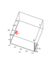
Finally, to complete our discussion, we show Figure 7. This figure shows the results of doing five iterations of the SVD-entropy based filtering and following that with three stages of DQC evolution. The dramatic clustering accomplished by DQC evolution makes it easy to extract clusters. Note however, that in the second plot we see what we have seen throughout, that the red points first form two distinct sub-clusters which only merge after two more stages of DQC evolution. This constant repetition of the same phenomenon, which is only made more apparent by SVD-entropy based filtering, is certainly a real feature of the data. It presumably says that what appears to be a sample of a single type of cell at the biological level is in reality two somewhat different types of cells when one looks at gene expression. A measure of the success of clustering is given by the Jaccard score which, for this result is $0.762$, higher than the value 0.707 obtained by [5].

5 DQC and Large Data Sets

There are many scientific and commercial fields, such as cosmology, epidemiology, particle physics, risk-management, etc., where the one deals with very large data sets, often in large numbers of dimensions. DQC, by its nature, doesn’t have trouble with large dimensions. In general it allows one to use SVD decomposition with much less severe dimensional reductions than other methods. However, dealing with large number of points requires some thought.

Since the method for evolving point requires diagonalizing the truncated Hamiltonian, and since diagonalizing such a matrix on a PC becomes difficult for matrices that are larger than $2000\times 2000$, it is obvious that using brute force methods to evolve sets of data having tens or hundreds of thousands of points simply won’t work. The solution to this problem lies in the fact that the SVD decomposition maps the data into an $N$-dimensional unit cube, and the fact that the data points are represented by states in Hilbert space rather than $N$-tuples of real numbers.

The key observation is that, since Gaussian wavefunctions whose centers lie within a given cube have non-vanishing overlaps, as one chooses more and more Gaussians one eventually arrives at a situation where the states become what we will refer to as essentially linearly dependent. In other words, we arrive at a stage at which any new wave-function added to the set can, to some predetermined accuracy, be expressed as a linear combination of the wave-functions we already have. Of course, since quantum mechanical time evolution is a linear process, this means that these additional states can be evolved by expressing them as linear combinations of the previously selected states and using the evolution of those states to evolve the extra states. Since computing the overlap of two Gaussians is done analytically determining which points determine the set of maximally essentially linearly independent states for the problem is easy. Typically, even for data sets with $100,000$ points, this is of the order of $1600$ points. The small number works because, as we have already noted, we don’t need high accuracy for DQC evolution. The quality of the clustering degrades very slowly with loss in accuracy. Thus, it is possible to compute the time evolution operator in terms of a well chosen subset of the data and then apply it to the whole set of points.

6 Afterward

Well this is about all I can cover in my allotted time. I hope I have convinced you that, strange as it may seem, quantum mechanics and data mining are related to one another. In fact, there is enough interest in this stuff in the real world that Stanford(SLAC) and Tel-Aviv University are patenting this technology and some companies have already expressed an interest in using it.

References

- [1] Marvin Weinstein and David Horn. Dynamic quantum clustering: a method for visual exploration of structures in data. SLAC-PUB-13759, arXiv-.0908.2644v1 [physics.data-an] 18 Aug 2009 (submitted to Phys. Rev. E)
- [2] D. Horn and A. Gottlieb. Algorithm for Data Clustering in Pattern Recognition Problems Based on Quantum Mechanics. Phys. Rev. Lett. 88 018702 (2001).
- [3] B. D. Ripley Pattern Recognition and Neural Networks. Cambridge University Press, Cambridge UK, 1996.
- [4] T.R. Golub, D.K. Slonim, P. Tamayo, C. Huard, M. Gaasenbeek et al: Molecular Classification of Cancer: Class Discovery and Class Prediction by Gene Expression Monitoring. Science 286 531 (1999).
- [5] R. Varshavsky, A. Gottlieb, M. Linial and D. Horn. Novel Unsupervised Feature Filtering of Biological Data. Bioinformatics 22 no. 14 (2006), e507-e513.