Evolution of the luminosity function

Abstract

The Smithsonian Hectospec Lensing Survey (SHELS) is a window on the star formation history over the last 4 Gyr. SHELS is a spectroscopically complete survey for $R_{\mathrm{tot}}<20.3$ over 4 □°. We use the 10k spectra to select a sample of pure star forming galaxies based on their emission line. We use the spectroscopy to determine extinction corrections for individual galaxies and to remove active galaxies in order to reduce systematic uncertainties. We use the large volume of SHELS with the depth of a narrowband survey for galaxies at $z\sim 0.24$ to make a combined determination of the luminosity function at $z\sim 0.24$. The large area covered by SHELS yields a survey volume big enough to determine the bright end of the luminosity function from redshift 0.100 to 0.377 for an assumed fixed faint-end slope $\alpha=-1.20$. The bright end evolves: the characteristic luminosity $L^{*}$ increases by 0.84 dex over this redshift range. Similarly, the star formation density increases by 0.11 dex. The fraction of galaxies with a close neighbor increases by a factor of $2-5$ for $L_{\ha}\gtrsim L^{*}$ in each of the redshift bins. We conclude that triggered star formation is an important influence for star forming galaxies with emission.

1 Introduction

Determining the star formation history of the Universe is a crucial part of understanding the formation and evolution of galaxies. Exploration of the global star formation history has two components: (i) measurement of the star formation density over time and (ii) understanding the physical processes that drive star formation. Here we use a large, moderate-depth spectroscopic survey to address both issues: (i) we determine the star formation density over the last 4 Gyr using the emission line as star formation indicator and (ii) we investigate the possible influence of galaxy interactions on the luminosity function.

There is abundant observational evidence for an order of magnitude increase in the star formation density since redshift $z\sim 1-2$ Lilly et al., 1996; Madau et al., 1996; and the compilations of Hopkins, 2004; Hopkins & Beacom, 2006. Major mergers, tidal interactions, gas removal from conversion into stars, and/or ram pressure stripping may explain the decrease in the star formation. The challenge is deciding which of these processes are important in quenching of star formation (Bell et al., 2005).

The decline in star formation density coincides with a rapid decrease in the characteristic luminosity of galaxies ($L^{*}$) in the rest-frame $U$-band (e.g. Ilbert et al., 2005; Prescott et al., 2009). A decrease in the number of merging systems can explain the decrease of the characteristic luminosity $L^{*}$ (Le Fèvre et al., 2000). Sobral et al. (2009) find a strong morphology- luminosity relation for mergers and non-mergers. The characteristic luminosity $L^{*}$ defines a critical switch-over luminosity between the mergers and non-mergers; the mergers are more luminous.

Studies of close pairs show that enhancement in the star formation rate is largest for galaxies in major pairs ($|\Delta m|\lesssim 0.7-2$; Woods et al., 2006; Woods & Geller, 2007; Ellison et al., 2008) and that the average star formation rate in a galaxy increases with decreasing projected separation (Li et al., 2008). Simulations of interacting and merging galaxies reveal that the interactions can trigger short powerful bursts of star formation by forcing substantial fractions of the gas into the central regions (Mihos & Hernquist, 1996).

Systematic effects dominate the comparison of star formation rates determined from different star formation indicators like the rest-frame ultra-violet (UV) and . Hence, to study the variation of the star formation density with time, the use of a single star formation indicator is best. The rest-frame UV spectrum of a galaxy directly measures the population of newborn stars (e.g. Lilly et al., 1996; Treyer et al., 1998). However, the rest-frame UV is strongly attenuated (e.g. Cardelli et al., 1989; Calzetti et al., 2000). The most-direct optical indicator is the emission line emitted by gas surrounding the embedded star forming region (e.g. Kennicutt, 1998). The line is also affected by attenuation–albeit less than the UV–which can be corrected using spectroscopy.

Many surveys use narrowband filters (Thompson et al., 1996; Moorwood et al., 2000; Jones & Bland-Hawthorn, 2001; Fujita et al., 2003; Hippelein et al., 2003; Ly et al., 2007; Pascual et al., 2007; Dale et al., 2008; Geach et al., 2008; Morioka et al., 2008; Shioya et al., 2008; Westra & Jones, 2008; Sobral et al., 2009) to determine the luminosity function parameters over a range of redshifts. Despite the depth of the narrowband surveys, measurements of individual luminosity function parameters and the star formation density are not well-constrained.

Narrowband surveys lack spectroscopy for the faint emitting galaxies. Thus, general assumptions about stellar absorption, extinction corrections, contributions by active galactic nuclei (AGNs), or interloper contamination need to be made for the sample as a whole rather than for each galaxy. These issues may lead to systematic uncertainties. Massarotti et al. (2001) show that applying an average extinction correction introduces a systematic underestimate of the extinction-corrected star formation density. A spectroscopic survey does not suffer these limitations, although it is usually limited in its depth.

Several spectroscopic surveys exist (e.g. Gallego et al., 1995; Tresse & Maddox, 1998; Sullivan et al., 2000; Tresse et al., 2002; Pérez-González et al., 2003; Shim et al., 2009). Both Gallego et al. and Pérez-González et al. use the Universidad Complutense de Madrid (UCM) survey. This survey covers an extremely wide area on the sky (472 □°). However, it is limited to a very low redshift ($z_{\mathrm{max}}\sim 0.045$). For their survey, Sullivan et al. (2000) use galaxies selected from UV imaging in a 2.2 □° field. The other surveys have an area $\leq$ 0.25 □°. Thus, most surveys are too limited in volume to overcome cosmic variance.

The Smithsonian Hectospec Lensing Survey (SHELS) is a spectroscopic survey covering 4 □° on the sky to a limiting $R$-band magnitude $R_{\mathrm{tot}}=20.3$ (Geller et al., 2005). We use SHELS to obtain a consistent determination of the star formation history over the last 4 Gyr based on the emission line over a relatively large area and redshift range.

The spectroscopy enables us to reduce systematic uncertainties by allowing an individual galaxy extinction correction. We can also remove individual AGNs rather than applying a global correction factor for contamination by AGNs as is done in narrowband surveys. We use the large survey area to determine the characteristic luminosity $L^{*}$ of the luminosity function and associated systematic uncertainties.

We discuss the SHELS spectroscopic data in Section 2. In Section 3 we introduce our sample selection. We combine our $R$-band selected sample with the narrowband survey of Shioya et al. (2008) in Section 4 to obtain a jointly-determined luminosity function at $z\sim 0.24$. Sections 5 and 6 discuss the derivation and evolution of the luminosity function and star formation density, respectively, over the past 4 Gyr. We include an investigation of the influence of our selection criteria on the derivation of the luminosity function parameters. In Section 7 we examine the stellar age of the star forming galaxies and the influence of galaxy-galaxy interactions on these galaxies. We summarize our results in Section 8.

Throughout this paper we assume a flat Universe with $H_{0}=71$ km s^-1 Mpc^-1, $\Omega_{\rm m}=0.27$ and $\Omega_{\Lambda}=0.73$. All quoted magnitudes are on the AB-system and luminosities are in erg s^-1.

2 SHELS observations

We constructed the SHELS galaxy catalog from the $R$-band source list for the F2 field of the Deep Lens Survey (Wittman et al., 2002, 2006). The DLS is an NOAO key program covering 20 □° in five separate fields; the 4.2 □° F2 field is centered at $\alpha=09^{h}19^{m}32.4^{s}$ and $\delta=+30\arcdeg{}00\arcmin{}00\arcsec{}$. We exclude regions around bright stars ($\sim$ 5 % of the total survey) resulting in an effective area of 4.0 □°. We use surface brightness and magnitude to separate stars from galaxies. This selection removes some AGN.

Photometric observations of F2 were made with the MOSAIC I imager (Muller et al., 1998) on the KPNO Mayall 4 m telescope between 1999 November and 2004 November. The $R$-band exposures, all taken in seeing $<0.9\arcsec{}$ FWHM, are the basis for the SHELS survey. The effective exposure time is about 14,500 seconds and the 1 $\sigma$ surface brightness limit in $R$ is 28.7 magnitudes per square arcsecond. Wittman et al. (2006) describe the reduction pipeline.

We acquired spectra for the galaxies with the Hectospec fiber-fed spectrograph (Fabricant et al., 1998, 2005) on the MMT from 2004 April 13 to 2007 April 20. The spectrograph is fed by 300 fibers that can be positioned over a 1° field. Roughly 30 fibers per exposure are used to determine the sky. The Hectospec observation planning software (Roll et al., 1998) enables efficient acquisition of a magnitude limited sample.

The SHELS spectra cover the wavelength range $\lambda=3,500-10,000$ Å with a resolution of $\sim$6 Å. Exposure times ranged from 0.75 hours to 2 hours for the lowest surface brightness objects in the survey. We reduced the data with the standard Hectospec pipeline (Mink et al., 2007) and derived redshifts with RVSAO (Kurtz & Mink, 1998) with templates constructed for this purpose (Fabricant et al., 2005). We have 1,468 objects that have been observed twice. These repeat observations imply a mean internal error of 56 km s^-1 for absorption-line objects and 21 km s^-1 for emission-line objects (see also Fabricant et al., 2005).

Fabricant et al. (2008) describe the technique we use for photometric calibration of the Hectospec spectra based on the particularly stable instrument response. For galaxies in common between SHELS and SDSS, the normalized line fluxes agree well in spite of the difference in fiber diameters for the Hectospec (1$\farcs$5) and the SDSS (3″). For high-signal-to-noise SHELS spectra, the typical uncertainties in emission line fluxes are 18 %.

SHELS includes 9,825 galaxies to the limiting apparent magnitude. The overall completeness of the redshift survey to a total $R$-band magnitude of $R_{\mathrm{tot}}\leq 20.3$ is 97.7 %, i.e. 9,595 galaxies have a redshift measured; the differential completeness at the limiting magnitude is 94.6 %. The 230 objects without redshifts are low surface and/or faint objects, or objects near the survey corners and edges. M. J. Kurtz et al. (2010; in preparation) includes a detailed description of the full redshift survey.

The SHELS survey also includes 1,852 galaxies with $20.3<R\leq 20.6$, for which we have measured a redshift; the total sample of galaxies with $20.3<R\leq 20.6$ is 3,590, i.e. the survey is 52 % complete in this magnitude interval. The completeness is patchy across the field.

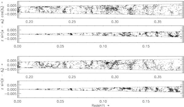
Figure 1: Redshift cone diagram for the galaxies in the final sample: $R_{\mathrm{tot}}\leq 20.3$, S/N${}_{\mathrm{\ha{}}}>5$ and $f_{\mathrm{\ha}}\geq 10^{-15.5}$ erg s^-1 cm^-2. AGNs have not been removed from this sample. The large-scale structure is apparent with extended low-density regions and well-populated narrow structures.

The F2 field contains an atypical under-dense region at the lowest redshifts because the DLS fields are selected against nearby clusters at $z<0.1$. We show the redshift distribution of our galaxies in Figure 1.

2.1 The $R$-band $k+e$-corrections

To calculate the absolute $R$-band magnitude $M_{R}$ we determine the appropriate $k+e$-corrections. The $k+e$-correction converts the observed absolute magnitude to the rest-frame of the galaxy, correcting for redshift and evolution. We use the $k+e$-corrections for 9 types of galaxies: bright cluster (BCG), elliptical (E), S0, Sa, Sb, Sbc, Sc, Sd and irregular (Irr) galaxies determined by J. Annis . We use the corrections for the SDSS $r^{\prime}$-filter as a function of redshift and $(g^{\prime}-i^{\prime})$-color because the SDSS $r^{\prime}$-filter is similar to the $R$-filter used for the DLS. We obtain $(g^{\prime}-i^{\prime})$ by cross-matching our catalog with SDSS DR6 (Adelman-McCarthy et al., 2008). For those galaxies not found in SDSS DR6 (these galaxies are either unresolved or below the surface brightness limit in SDSS) we convert the $(V-R)$ from 61 galaxies in the DLS to $(g^{\prime}-i^{\prime})$. For 42 galaxies we cannot determine or derive $(g^{\prime}-i^{\prime})$ due to the proximity of another object; we assume that these are Sa galaxies. We interpolate the models in redshift to obtain the $k+e$-corrections for each galaxy type determined by its $(g^{\prime}-i^{\prime})$ and redshift.

3 sample selection

We use SHELS to construct luminosity functions over the redshift range $0.010<z<0.377$ (Table 1). Here, we describe the determination of our final emission-line luminosities and the discrimination between pure star-forming galaxies and AGNs.

3.1 Emission-line measurements

The emission-line flux emanating from star-forming regions is affected by the absorption-line spectrum from the underlying stellar population. The absorption mostly affects the measurements of the hydrogen Balmer lines. To measure the emission-line flux we thus remove the contribution of the stellar population.

We use the Tremonti et al. (2004) continuum subtraction method to correct for the stellar absorption rather than applying a constant, global correction (e.g., Hopkins et al., 2003). The Tremonti et al. method removes the stellar continuum by fitting a linear combination of template spectra resampled to the correct velocity dispersion. The method also accounts for redshift and reddening. The template spectra are based on single stellar population models generated by the population synthesis code of Bruzual & Charlot (2003). We use models with 10 different ages (0.005, 0.025, 0.1, 0.3, 0.6, 0.9, 1.4, 2.5, 5 and 10 Gyr) at solar metallicity.

We determine the emission-line fluxes from the continuum-subtracted spectra by integrating the line flux within a top-hat filter centered on the emission-line. We remove any local over- or under-subtraction of the continuum by subtracting the mean of the flux-density at both sides of the filter. Next, we determine the continuum level by taking the mean of the flux-density at wavelengths bluer and redder than the emission-line on the best-fit continuum model. Finally, we determine the absorption contribution of the underlying stellar population using the same top-hat filter but on the best-fit model; we remove the flux contributed by the continuum.

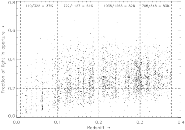
Figure 2: Fraction of light contained in the 1$\farcs$5 fibers as a function of redshift. We indicate the fraction of galaxies with more than 20 % of the light contained in the fiber (horizontal dashed line) for each redshift bin (vertical dashed lines) we use to construct the luminosity functions. The galaxies have $R_{\mathrm{tot}}\leq 20.3$, S/N${}_{\mathrm{\ha{}}}>5$ and $f_{\mathrm{\ha}}\geq 10^{-15.5}$ erg s^-1 cm^-2. The AGNs have been removed.

The Hectospec fibers have a fixed diameter of 1$\farcs$5. At all redshifts where is observable (and in particular at the lowest redshifts) the fiber does not cover the entire galaxy. Hence, we use an aperture correction

$$A=10^{-0.4(m_{\mathrm{total}}-m_{\mathrm{fiber}})}$$ (1)

to correct for the fiber-covering fraction. Figure 2 shows the fraction of light, $1/A$, contained in the fiber as a function of redshift.

Kewley et al. (2005) show that a spectrum measuring at least 20 % of the galaxy light avoids substantial scatter between the nuclear and integrated SFR measurements. The overall majority of galaxies from SHELS have a light-fraction $1/A\geq 20\,\%$ (Figure 2).

Fabricant et al. (2008) compared the and [Oii] emission-line fluxes from SHELS with SDSS DR6 after making an aperture correction. They found excellent agreement between the two surveys, even though the fibers of the SDSS spectrograph are 3″ in diameter. Moreover, most of the SDSS galaxies are at low redshift ($z\lesssim 0.14$) where we have the largest fraction of galaxies with a light-fraction less than 20 %.

There is no dependence of final luminosity on the light-fraction. We are thus confident that the use of these aperture corrections does not affect the final results even when the covering fraction is small.

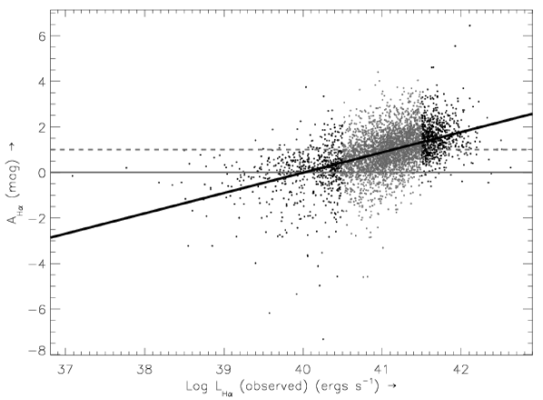
Figure 3: Attenuation at as function of observed luminosity. The black line indicates the least-absolute-deviates fit to the gray points. We indicate $A_{\ha}{}=0$ (solid horizontal line) and a commonly assumed value of $A_{\mathrm{\ha}}$ ($A_{\mathrm{\ha}}=1$, dashed horizontal line; e.g. Tresse & Maddox, 1998; Fujita et al., 2003; Ly et al., 2007; Sobral et al., 2009)

3.2 Extinction correction

The light from star forming regions in a galaxy is often heavily attenuated. To determine the intrinsic SFR of a galaxy we must remove the effects of attenuation.

We calculate the attenuation by comparing the observed value of the Balmer decrement (corrected for stellar absorption) with the theoretical value ($f_{\ha}/f_{\mathrm{H\beta}}=2.87$ for $T\,=\,10^{4}$ K and case B recombination; Table 2 of Calzetti, 2001). The intrinsic flux is $f_{\mathrm{intr}}(\lambda)=f_{\mathrm{obs}}(\lambda)10^{0.4A_{\lambda}}$, where $A_{\lambda}$ is the wavelength-dependent extinction. $A_{\lambda}$ is

$$A_{\lambda} = k(\lambda)E(B-V)_{\mathrm{gas}}$$ (2)

$$= k(\lambda)\frac{2.5\log R_{\alpha\beta}}{k({\mathrm{H\beta}})-k(\ha)}~{},$$

where $R_{\alpha\beta}$ is the ratio of the attenuated-to-intrinsic Balmer line ratios, $k({\mathrm{H\beta}})-k(\ha)$ is the differential extinction between the wavelengths of H$\beta$ and , and $k(\lambda)$ is the extinction at wavelength $\lambda$. We apply the Calzetti et al. (2000) extinction law, which has $k(V)=4.05$, $k(\ha)=3.325$ and $k({\mathrm{H\beta}})=4.596$.

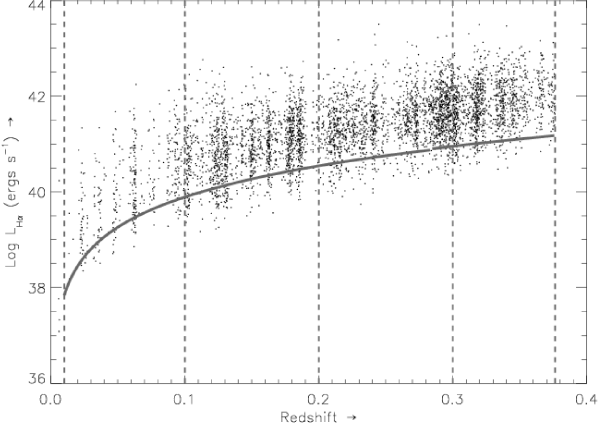
Figure 4: luminosity (corrected for extinction) as a function of redshift. The solid line indicates the additional selection criterion $f_{\mathrm{\ha}}\geq 10^{-15.5}$ erg s^-1 cm^-2. Vertical dashed lines show the edges of the redshift bins used to construct the SHELS luminosity functions.

Figure 3 shows the attenuation as a function of observed luminosity for galaxies with both and H$\beta$ at a $\mathrm{S/N}>5$. We use the relation between $A_{\ha}{}$ and $L_{\ha}{}$ as determined from a least-absolute-deviates fit to the high-S/N data-points with observed luminosities $40.5<\log L_{\mathrm{\ha}}<41.5$ (gray points) for galaxies where $\mathrm{S/N}_{\mathrm{{\mathrm{H\beta}}}}\leq$ 5 or where the observed equivalent width of H$\beta$, OEW${}_{\mathrm{{\mathrm{H\beta}}}}\leq$ 1 Å (uncorrected for stellar absorption). We limit OEW_Hβ to avoid galaxies with excessively large attenuation resulting from a very small (noise-dominated) H$\beta$ flux compared to . We assume that galaxies with $A_{\ha}{}\leq 0$ to have no attenuation and assign $A_{\ha}{}=0$ to these galaxies.

3.3 Sample definition

Figure 4 shows the luminosity as a function of redshift. Below $f_{\mathrm{\ha}}=10^{-15.5}$ erg s^-1 cm^-2 the number of galaxies decreases rapidly. We impose a constant flux limit $f_{\mathrm{\ha}}\geq 10^{-15.5}$ erg s^-1 cm^-2 on the sample (after corrections for stellar absorption and attenuation) because we are only complete to this flux. We apply this criterion in addition to the magnitude limit ($R_{\mathrm{tot}}\leq 20.3$) and the $\mathrm{S/N}_{\mathrm{\ha}}>5$ requirement.

3.4 AGN classification

The presence of an active nucleus in a galaxy contributes to the (apparent) star-formation in the galaxy. For example, Pascual et al. (2001) find that approximately 15 % of the luminosity density of the UCM survey (Gallego et al., 1995) results from galaxies identified as AGN. Westra & Jones (2008) find a 5 % contribution for their survey.

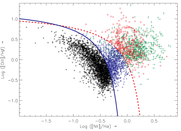
Figure 5: BPT (after Baldwin et al., 1981) diagram for SHELS. The solid blue and dashed red lines indicate the demarcation of pure star formation from Kauffmann et al. (2003) and of extreme starbursts from Kewley et al. (2001). We classify the galaxies as: pure star forming galaxies (black diamonds), AGNs (red squares), and composite galaxies (blue triangles). We indicate galaxies or AGNs with either or H$\beta$ undetected, i.e. $\mathrm{S/N}<3$, as lower limits (green arrows).

We use the demarcations of pure star formation from Kauffmann et al. (2003) and of extreme starburst from Kewley et al. (2001) to identify galaxies as pure star forming, AGN, or a combination (composite galaxies) based on the line ratios of [O iii]/H$\beta$ and [N ii]/ (Figure 5).

We select all galaxies with [O iii] $\lambda$5007 and [N ii] $\lambda$6585 detected with a signal-to-noise ratio (S/N) $\geq 3$. If the galaxies have both and H$\beta$ detected with S/N $\geq 3$, we identify them as pure star forming galaxies when their line ratios are below the Kauffmann et al. relation, pure AGNs when the ratios are above the Kewley et al. relation, and composites when they lie between the relations.

For galaxies with either or H$\beta$ undetected (S/N $<$ 3), we use the 3 $\sigma$ value for the line flux to calculate the line ratios. These ratios are lower limits. We classify these galaxies as composite or AGN; some of the composite galaxies might be AGNs.

We identify a separate class of broad-line AGN. The width of these broad Balmer-lines extends beyond the limited-width top-hat filter used for measuring the line fluxes (Section 3.1). In some cases the [N ii] $\lambda\lambda$6550,6585 lines are not distinguishable from the line in a spectrum with a very broad line.

Inspecting each spectrum would be time-consuming. Hence, we fit the and H$\beta$ lines in the continuum-subtracted spectra in an automated way and individually inspected each candidate broad-line AGN. We fit both lines simultaneously with the assumption that the full-width-half-maximum (FWHM) of the line profile is the same for both lines. Candidate broad-line AGNs have a peak of both and H$\beta$ $>5\times 10^{-18}$ erg s^-1 cm^-2 Å^-1 above the continuum residuals (which avoids the inclusion of noise peaks) and a FWHM of the Gaussian component of the line profile (we use a Gaussian convolved with the instrumental profile as our line profile) before convolution larger than 14 Å. From these candidates, we select the galaxies that are genuine broad-line AGNs.

The fraction of galaxies identified as AGN and/or composite over the redshift ranges 0.010-0.100, 0.100-0.200, 0.200-0.300 and 0.300-0.377 for an luminosity limited sample ($\log L\geq 41.18$; lowest luminosity at $z=0.377$) is 5.9, 6.6, 5.3 and 5.2 %, respectively.

The fraction of AGN is more or less constant with redshift. However, we cannot draw any conclusions about the evolution of the AGN-fraction as a function of redshift. We removed stellar objects from the initial sample and thus may have inadvertently removed AGNs particular at greater redshifts.

4 The luminosity function at redshift $\sim$ 0.24

The recent advent of wide-field cameras on telescopes has aided searches for star forming galaxies by increasing the area (and hence volume) of narrowband surveys, e.g. Fujita et al. (2003), Ly et al. (2007), Shioya et al. (2008), Westra & Jones (2008), and many more. This technique has recently been extended to the near-infrared, e.g. Sobral et al. (2009).

A narrowband survey efficiently probes the faint end of the luminosity function which is hard to explore in a spectroscopic survey. In contrast, a spectroscopic survey can cover a larger volume and sample the rare luminous galaxies at the bright end of the luminosity function.

Here, we combine the strength of a narrowband survey–the ability to go deep–with that of our broadband selected spectroscopic survey–coverage of a large volume–to determine a well-constrained luminosity function at $z\sim 0.24$. For the narrowband survey we use the publicly available data from Shioya et al. (2008, hereafter S08) together with that of the Cosmic Evolution Survey (COSMOS; Capak et al., 2007) which formed the basis of the survey of S08. We use the spectroscopic survey of SHELS for the bright end of the luminosity function.

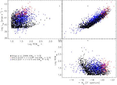
Figure 6: Comparison of SHELS with S08 for galaxies with the OEW${}_{\ha+{\mbox{[{\sc N\,ii}]}}}>12$ Å not corrected for [N ii] for both surveys. The data are: S08 (solid black circles), SHELS in the redshift range of S08 (open red squares), and SHELS at $0.01<z<0.15$ (open blue triangles). The luminosity, $L_{\ha}$, for both surveys is corrected for [N ii].

The S08 and SHELS surveys use different approaches (imaging versus spectroscopy). A comparison of the data allows a consistency check of the aperture corrections applied to the SHELS data.

We construct the luminosity function over the redshift range of S08 ($0.233<z<0.251$) based on the catalog with emission-line fluxes determined in Section 3.1 (which already include corrections for underlying stellar absorption), redshifts, extinction corrections from Section 3.2, and removal of composites and AGNs (Section 3.4). Constraining SHELS to the same redshift range yields a sample of 192 SHELS galaxies at $0.233<z<0.251$.

4.1 Data comparison

Figure 6 shows the luminosity, rest-frame equivalent width (REW), and the 3″ aperture absolute $R$-band magnitude from S08 (solid black circles) matched to the selection criteria of SHELS, $R_{\mathrm{tot}}\leq 20.3$. We also show the SHELS data (open red squares) for the redshift range covered by S08 ($0.233<z<0.251$). To match S08 we require an observed equivalent width of combined with [N ii] $\geq 12$ Å (as per the selection criteria of S08), and $f_{\mathrm{\ha}}\geq 10^{-15.5}$ erg s^-1 cm^-2. The strengths of both surveys are immediately apparent. SHELS includes the highest luminous galaxies, S08 probes the faint end of the luminosity function.

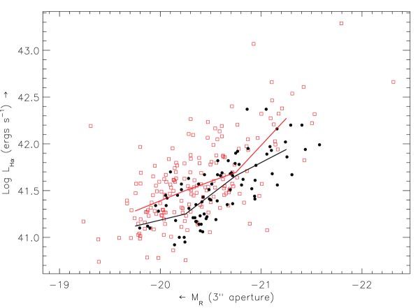
Figure 7: Comparison of the total luminosity with the 3″ aperture $R$-band magnitude of SHELS (open red squares) and the survey of S08 (solid black circles). The galaxies have OEW${}_{\mathrm{\ha+{\mbox{[{\sc N\,ii}]}}}}\geq 12$ Å, a flux-limit of $f_{\mathrm{\ha}}\geq 10^{-15.5}$ erg s^-1 cm^-2, $R_{\mathrm{tot}}\leq 20.3$, and $0.233<z<0.251$. We show the median luminosity for 0.5 magnitude-wide bins for SHELS (red line) and S08 (black line). The SHELS galaxies shift toward greater $L_{\mathrm{\ha}}$ at fixed $M_{R}$

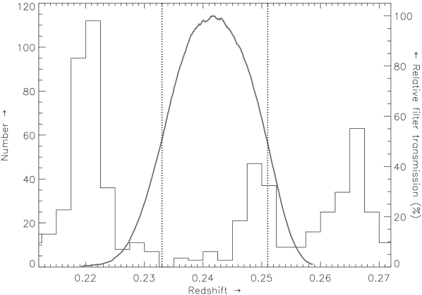
Figure 8: Redshift distribution of the galaxies in zCOSMOS DR2 (Lilly et al., 2007, histogram), the relative NB816 filter transmission curve used by S08 (gray solid line), and where the transmission of the NB816 filter is 50 % of its maximum (dotted lines).

S08 measure magnitudes from a 3″ aperture, scale them to the total $i^{\prime}$-band magnitude, and calculate fluxes. We measure fluxes in a similar way. We use spectra taken with a 1$\farcs$5-fiber aperture scaled to the total $R$-band magnitude. The data from the lower redshift range $0.01<z<0.15$ of SHELS (Figure 6; open blue triangles) show that the relation between the luminosity and the 3″ total $R$-band magnitude of the two surveys is similar. The scaling of the flux from the limited-aperture magnitude to the total magnitude introduces no systematic biases and is consistent with S08.

If we constrain the data of S08 to $f_{\mathrm{\ha}}=10^{-15.5}$ erg s^-1 cm^-2, a difference at the bright end becomes apparent (see Figure 7). There are more-luminous galaxies in SHELS than in S08. This difference results from two effects: (i) SHELS probes a larger volume, and (ii) the fluxes determined from narrowband surveys can easily underestimate the true line flux. Galaxies with redshifts that place the line in the wings of the filter underestimate the mean recovered flux.

To examine the redshift distribution of the galaxies in S08, Figure 8 shows the redshift distribution of the 10k zCOSMOS catalog (Lilly et al., 2007) in combination with the filter transmission curve of the NB816 normalized to the maximum throughput. Any galaxy with a redshift placing it in the wings of the narrowband filter has its flux underestimated far more than the 21 % S08 use to correct their line fluxes. In the COSMOS field the galaxies tend to be at redshifts towards the red edge of the filter. In this case, the [N ii] $\lambda$6585 line (the strongest of the two [N ii] lines that straddle ) barely contributes to the flux probed by the filter. Both the underestimation of the flux and over-correction for [N ii] can explain the difference in the distribution of fluxes in Figure 7.

Despite this difference, we can still use the fainter galaxies from S08 to determine the faint-end slope of the luminosity function. The systematic underestimation of fluxes causes a shift in the luminosity function which affects the determination of the characteristic luminosity (i.e. bright end), not the faint-end slope.

4.2 Derivation and fit

We fit a Schechter function (Schechter, 1976) to the SHELS and S08 data. The Schechter function is

$$\phi(L)dL=\phi^{*}\left(\frac{L}{L^{*}}\right)^{-\alpha}\exp\left(-\frac{L}{L^{*}}\right)d\left(\frac{L}{L^{*}}\right),$$ (3)

where $\alpha$ is slope of the faint-end part, $L^{*}$ is a characteristic luminosity, and $\phi^{*}$ is the normalization. Throughout this paper the units for the Schechter parameters $L^{*}$ and $\phi^{*}$ are erg s^-1 and Mpc^-3, respectively. $\alpha$ is dimensionless.

To combine the two data sets we use the non-parametric 1/V_max method (Schmidt, 1968) to determine the Schechter parameters. The number density of galaxies for each luminosity bin $j$ with a width of $\Delta\log L$ is

$$\phi(L_{j})\Delta\log L=\sum\limits_{i=1}^{N_{\mathrm{gal}}}\frac{W(L_{i})}{V_{i}},$$ (4)

where $W(x)=1$ when the luminosity is enclosed by bin $j$ and $W(x)=0$ otherwise, and $V_{i}$ is the volume sampled by galaxy $i$. The uncertainties in the bins are Poisson errors

$$\sigma^{2}_{\phi(L_{j})}=\sum\limits_{i=1}^{N_{\mathrm{gal}}}\frac{W(L_{i})}{V_{i}}.$$ (5)

Figure 9: The 1/V_max data-points for SHELS (solid squares), SHELS without the OEW${}_{\mathrm{\ha+{\mbox{[{\sc N\,ii}]}}}}\geq 12$ Å criterion (solid diamonds), and S08 (open squares). The galaxies have OEW${}_{\mathrm{\ha+{\mbox{[{\sc N\,ii}]}}}}\geq 12$ Å, $R_{\mathrm{tot}}\leq 20.3$, and $0.233<z<0.251$. The thick solid line indicates the combined fit of SHELS and S08 with $\phi^{*}_{\mathrm{comb}}=-3.05\pm 0.09$, $\alpha=-1.41\pm 0.03$, and $\log L^{*}=42.14\pm 0.08$. The thin lines indicate the luminosity function for the SHELS and S08 data separately with $\phi^{*}_{\mathrm{SHELS}}=-3.11\pm 0.09$ (dashed line) and $\phi^{*}_{\mathrm{S08}}=-2.91\pm 0.09$ (dotted line), respectively. Both luminosity functions also have $\alpha=-1.41\pm 0.03$ and $\log L^{*}=42.14\pm 0.08$.

Figure 9 shows the luminosity function for the combined data set (thick solid line). For both surveys we apply the selection criteria $R_{\mathrm{tot}}\leq 20.3$, OEW${}_{\mathrm{\ha+{\mbox{[{\sc N\,ii}]}}}}\geq 12$ Å, and $0.233<z<0.251$.

We determine the data-points using 1/V_max where the uncertainties are Poisson errors for both SHELS (solid squares) and S08 (open squares). We fit a Schechter function with common $L^{*}$ and $\alpha$ to the combined SHELS and S08 dataset. For this fit, we use the data with $\log L_{\ha}{}\geq 41.4$ for SHELS and $\log L_{\ha}{}\geq 39.6$ for S08. We recover a single value for $\alpha$ and $L^{*}$ of the joint fit: $\alpha=-1.41\pm 0.03$ and $\log L^{*}=42.14\pm 0.08$. For those values, the normalization for SHELS is $\log\phi^{*}_{\mathrm{SHELS}}=-3.11\pm 0.09$ and for S08 is $\log\phi^{*}_{\mathrm{S08}}=-2.91\pm 0.09$. We combine $\phi^{*}_{\mathrm{S08}}$ and $\phi^{*}_{\mathrm{SHELS}}$ using a volume-weighted average. Thus, $\log\phi^{*}_{\mathrm{comb}}=\log[(1.5\times 10^{-2.91}+4.0\times 10^{-3.11})/5.5]=-3.05$. This method of combining is one way to account for cosmic variance. We adopt $\alpha=-1.41\pm 0.03$, $\log L^{*}=42.14\pm 0.08$, $\log\phi^{*}_{\mathrm{comb}}=-3.05\pm 0.09$ for comparison to other surveys.

5 The luminosity functions from SHELS

Table 1: Number of galaxies satisfying each selection criterion.

Criterion		$0.01\leq z<0.10$	$0.10\leq z<0.20$	$0.20\leq z<0.30$	$0.30\leq z<0.38$	Total
(i)	$R_{\mathrm{tot}}\leq 20.3$	461	1949	2746	2114	7270
(ii)	$\mathrm{S/N}_{\mathrm{\ha}}>5$	420	1640	1857	1275	5192
(iii)	$\log_{\mathrm{\ha}}\geq-15.5$	369	1441	1702	1186	4698
(iv)	pure star forming	322	1127	1268	0848	3565

Note. — Successive lines are a subset of the line above. We apply the selection criteria sequentially in the order of the Table.

Here we use SHELS to determine the luminosity functions as a function of redshift. We can identify in our spectra up to a redshift of $z_{\mathrm{max}}=0.377$. We next examine the influence of the $R$-magnitude limited survey on the derivation of the luminosity function. We limit our sample to $f_{\mathrm{\ha}}\geq 10^{-15.5}$ erg s^-1 cm^-2 (see Section 3.3). Table 1 lists the number of galaxies satisfying each selection criterion. Figure 4 shows the distribution of the luminosity as a function of redshift and the redshift bins used to construct the luminosity functions.

5.1 Derivation and fit

Here we use the STY-method (Sandage et al., 1979), a parametric estimation method, to determine the three Schechter parameters for each redshift bin. The STY-method identifies the luminosity function parameters that maximize the probability of obtaining the observed sample. The probability $\mathcal{P}$ is

$$\mathcal{P}=\prod\limits_{i=1}^{N_{\mathrm{gal}}}\frac{\phi(L_{i})}{\int^{\infty}_{L(z_{i})_{\mathrm{lim},i}}\phi(L)dL},$$ (6)

where $L(z)_{\mathrm{lim},i}$ is the faintest luminosity where galaxy $i$ at redshift $z_{i}$ is observable. We use a truncated-Newton method to maximize the natural logarithm of $\mathcal{P}$.

Figure 10: luminosity functions for several redshift bins for our pure star forming sample. The Schechter functions are derived using the STY-method with $\alpha$ fixed to $-1.2$. The data-points come from 1/V_max where the uncertainties are Poisson errors. Table 2 lists the parameters.

Table 2 lists the fit-parameters, and Figure 10 shows the results. We fit for $\alpha$, $L^{*}$, and $\phi^{*}$ (dashed lines). We also use a fixed $\alpha=-1.20$ (solid lines). This fixed value represents the slope over the redshift range $0.05<z<0.20$ for SHELS. This range has a large enough volume to sample the bright end of the luminosity function, while still having galaxies faint enough to determine the faint end slope. We do not consider this large redshift range in our further analysis.

Narrowband surveys apply a correction to the total luminosity density for galaxies hosting an AGN (e.g. Fujita et al., 2003; Ly et al., 2007; Shioya et al., 2008; Westra & Jones, 2008). A large fraction of these surveys have little or no spectroscopy. Thus there is no way to separate AGNs from star forming galaxies. SHELS enables a direct separation (see Section 3.4). We derive the Schechter parameters for the emitting galaxies with the AGNs removed (Table 2). Removal of AGNs moves $L^{*}$ slightly fainter and reduces the normalization because AGNs are systematically in more luminous galaxies. Failure to account for this bias introduces a systematic offset.

Table 2: Parameters for the luminosity functions.

	fixed $\alpha$			unconstrained $\alpha$
redshift range	$\alpha$	$\log L^{*}$	$\log\phi^{*}$	$\alpha$	$\log L^{*}$	$\log\phi^{*}$
Pure star forming sample
$0.010<z<0.100$	$-1.20$	$41.72\pm 0.10$	$-2.86\pm 0.04$	$-1.22\pm 0.06$	$41.74\pm 0.13$	$-2.90\pm 0.10$
$0.100<z<0.200$	$-1.20$	$42.09\pm 0.04$	$-2.97\pm 0.02$	$-0.87\pm 0.05$	$41.79\pm 0.06$	$-2.58\pm 0.05$
$0.200<z<0.300$	$-1.20$	$42.52\pm 0.04$	$-3.29\pm 0.01$	$-0.71\pm 0.07$	$42.13\pm 0.06$	$-2.79\pm 0.05$
$0.300<z<0.377$	$-1.20$	$42.83\pm 0.03$	$-3.59\pm 0.01$	$-0.50\pm 0.06$	$42.30\pm 0.05$	$-2.96\pm 0.04$
$0.233<z<0.251$				$-1.41\pm 0.03$	$42.14\pm 0.08$	$-3.05\pm 0.09$
Pure star forming sample including composites and AGNs
$0.010<z<0.100$	$-1.20$	$41.76\pm 0.10$	$-2.82\pm 0.04$	$-1.25\pm 0.06$	$41.85\pm 0.13$	$-2.93\pm 0.10$
$0.100<z<0.200$	$-1.20$	$42.13\pm 0.04$	$-2.88\pm 0.02$	$-0.99\pm 0.05$	$41.92\pm 0.06$	$-2.61\pm 0.05$
$0.200<z<0.300$	$-1.20$	$42.55\pm 0.04$	$-3.17\pm 0.01$	$-0.88\pm 0.07$	$42.26\pm 0.06$	$-2.80\pm 0.05$
$0.300<z<0.377$	$-1.20$	$42.83\pm 0.03$	$-3.44\pm 0.01$	$-0.66\pm 0.06$	$42.39\pm 0.05$	$-2.90\pm 0.04$

Note. — For each redshift range, we list the determined Schechter parameters with fixed $\alpha=-1.20$ (left) and $\alpha$ unconstrained (right) and their uncertainties. We also list the parameters for the Schechter fit for a pure star forming sample (top) and a sample where the AGNs and composites are included (bottom). The pure star forming sample and the sample including composites and AGNS are based on criterion (iv) and (iii), respectively, in Table 1. The quoted uncertainties are calculated in Section 5.1.

Figure 11: The distributions of $\log L_{\ha}$ as function of $M_{R}$ for each redshift bin. We use these distributions to assign an luminosity to the observed absolute magnitude and to assign an absolute magnitude to a simulated luminosity. This procedure enables us to determine the final uncertainties in the Schechter parameters and to study the influence of the survey selection criterion $R_{\mathrm{tot}}\leq 20.3$.

We determine the final uncertainties in the Schechter parameters by constructing 1,000 sets of luminosities. We simulate the luminosities by converting the observed absolute magnitudes into luminosities using the distribution of $L_{\ha}{}$ as a function of $M_{R}$ for each redshift bin from Figure 11. We redetermine the Schechter parameters for each simulation using the STY-method. The 1 $\sigma$ spread in the redetermined parameters is the final uncertainty which includes the formal fitting uncertainty, uncertainties resulting from the size of the sampled volume, and the uncertainties in the observed luminosity. Table 2 lists the Schechter parameters and their uncertainties.

Figure 12: The three Schechter parameters as a function of redshift and look-back time for SHELS for pure star forming galaxies (red, green, blue, and cyan points), SHELS combined with S08 (magenta point), and surveys at similar redshifts that also use as star formation indicator (black points).

5.2 Parameter evolution and impact of selection criteria

Figure 12 compares the Schechter function parameters of SHELS with fixed $\alpha=-1.20$ with other surveys. Evolution in the characteristic luminosity $L^{*}$ is clearly visible.

The selection of galaxies by apparent $R$-band magnitude does not yield the same sample of galaxies obtained when selecting by flux/luminosity. Because we determine the luminosity function from an $R$-selected spectroscopic survey, we must investigate the potential systematic effects of the selection criteria ($R_{\mathrm{tot}}\leq 20.3$ and $f_{\mathrm{\ha}}\geq 10^{-15.5}$ erg s^-1 cm^-2) on the luminosity function.

From a given luminosity function ($\alpha=-1.20$, $\log L^{*}({\mathrm{erg\,s^{-1}}})=42.00$, and $\log\phi^{*}({\mathrm{Mpc^{-3}}})=-2.75$) we construct a sample of galaxies with a flux $f_{\mathrm{\ha}}\geq 10^{-15.5}$ erg s^-1 cm^-2. We choose these parameters because they are close to our recovered parameters from SHELS. Furthermore, we keep the parameters constant over our redshift range to test whether our selection criteria introduce an artificial evolution to the parameters. We assume a uniform galaxy distribution in a comoving volume. We assign each simulated galaxy an absolute magnitude using the distribution of absolute magnitude as function of $L_{\mathrm{\ha}}$ in Figure 11. We calculate the apparent magnitude using the allocated redshift and a $k+e$-correction based on the observed distribution as a function of redshift. We apply the survey selection criterion of $R_{\mathrm{tot}}\leq 20.3$ and recover the Schechter parameters using the STY-method. Figure 13 and Table 3 give the results.

Table 3: Recovered Schechter parameters for simulated luminosity functions.

	fixed $\alpha$			unconstrained $\alpha$
redshift range	$\alpha$	$\log L^{*}$	$\log\phi^{*}$	$\alpha$	$\log L^{*}$	$\log\phi^{*}$
input parameters	$-1.20$	$42.00$	$-2.75$	$-1.20$	$42.00$	$-2.75$
$0.010\leq z<0.100$	$-1.20$	$42.01\pm 0.07$	$-2.75\pm 0.02$	$-1.18\pm 0.04$	$41.98\pm 0.10$	$-2.71\pm 0.08$
$0.100\leq z<0.200$	$-1.20$	$42.06\pm 0.03$	$-2.77\pm 0.01$	$-1.07\pm 0.03$	$41.93\pm 0.04$	$-2.60\pm 0.04$
$0.200\leq z<0.300$	$-1.20$	$42.18\pm 0.02$	$-2.84\pm 0.01$	$-0.73\pm 0.05$	$41.85\pm 0.03$	$-2.43\pm 0.03$
$0.300\leq z<0.377$	$-1.20$	$42.33\pm 0.02$	$-2.95\pm 0.01$	$-0.17\pm 0.07$	$41.81\pm 0.03$	$-2.38\pm 0.01$

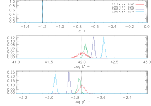
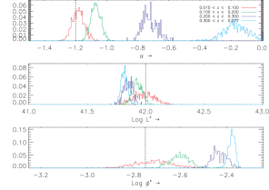
Figure 13: Histogram of the luminosity function parameters determined from simulations to test the influence of the $R$-band selection criteria on the luminosity function. Each histogram (red, green, blue, cyan) indicates the recovered parameters for a different redshift bin. Vertical dotted lines indicate the input parameters of the luminosity function to the simulations ($\alpha=-1.20$, $\log L^{*}=42.00$, and $\log\phi^{*}=-2.75$). We indicate the results with $\alpha$ fixed at $-1.20$ (left) and with $\alpha$ as a free parameter (right). Table 3 also shows the results.

When we keep $\alpha$ fixed in fitting the simulations, there is an artificial trend of increasing $L^{*}$ and decreasing $\phi^{*}$ with increasing redshift. This trend results from selective removal of the fainter galaxies. The removal would otherwise result in $\alpha$ decreasing (which we also show for $\alpha$ unconstrained). Thus, $L^{*}$ and $\phi^{*}$ should be corrected for the fact that $\alpha$ is kept fixed at a steeper value than would be fit. However, the simulated trend in $L^{*}$ and $\phi^{*}$ is far smaller ($\Delta\log L^{*}=0.33$, $\Delta\log\phi^{*}=-0.20$) than we determine from the observations ($\Delta\log L^{*}=1.11$, $\Delta\log\phi^{*}=-0.73$). Thus, the evolution in $L^{*}$ in Figure 12 is real.

When we fit the simulations for all three parameters (unconstrained $\alpha$ in Table 3), the decrease of $\alpha$ ($\Delta\alpha=-1.01$) with increasing redshift is close to that of the observations ($\Delta\alpha=-0.72$; Table 2). Moreover, the faint-end slope from our lowest redshift bin ($0.010<z<0.100$; where the faint-end of the luminosity function is well-sampled) is consistent with that of the combined luminosity function of SHELS and S08 at $z\sim 0.24$ (Section 4.2) within the uncertainties. Hence, we have no evidence for evolution of the faint-end slope over the redshift range covered by SHELS. The trend observed with the faint-end slope unconstrained is the result of our selection criteria.

We also notice an artificial trend in $L^{*}$ with increasing redshift for a constant luminosity function (although smaller than with $\alpha$ constrained) opposite to the trend observed, and opposite to the trend we derive fitting for $\alpha=-1.20$. To compensate for a shallow faint-end slope and a slight decrease in $L^{*}$ with redshift, $\phi^{*}$ increases in these simulations.

We do not consider $\phi^{*}$ because it only normalizes the luminosity function and does not determine the shape of it, unlike $\alpha$ and $L^{*}$. The normalization is dependent on the number of galaxies sampled. Because this number is heavily influenced by the distribution of galaxies (i.e. the large-scale structure, see Figure 4), it is not possible to say anything meaningful about any trend in $\phi^{*}$ even with the area covered by SHELS.

In summary, there is strong evidence for evolution in $L^{*}$ and no evidence for evolution in $\alpha$ over $0.100<z<0.377$.

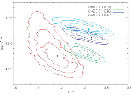
Figure 14: The luminosity function parameters for the input luminosity function used to determine the observed luminosity functions as shown in Figure 10. The contours show the 68.3, 95.4, and 99.7 % confidence intervals based on the fit of the output luminosity function.

5.3 The “true” luminosity function

In Section 5.2 we investigate the influence of our selection criteria on an assumed luminosity function. We can extend this application to determine the “true” luminosity function.

We construct a sample of galaxies with a flux $f_{\mathrm{\ha}}\geq 10^{-15.5}$ erg s^-1 cm^-2 for a grid of given values of $\alpha$ and $L^{*}$. We constrain $\phi^{*}$ by the number of observed galaxies in each redshift bin. These choices are our input Schechter parameters. We apply our magnitude selection of $R_{\mathrm{tot}}\leq 20.3$. Then we determine the output: the parameters one would recover using the STY-method. We take the median of the recovered Schechter parameters as our final output Schechter parameters. With these final output parameters we determine the likelihood for our observations (Figure 10). We also show the input parameters and the confidence intervals from the likelihood-determination for each redshift bin (Figure 14).

Again, we find a significant evolution of $L^{*}$. $L^{*}$ increased towards higher redshifts, regardless of the inclusion of the lowest redshift results. Furthermore, there is no significant evolution in the faint end slope of the intrinsic luminosity function. These results confirm the findings in the Section 5.2. The evolution in $L^{*}$ is real and there is no evidence for evolution in $\alpha$.

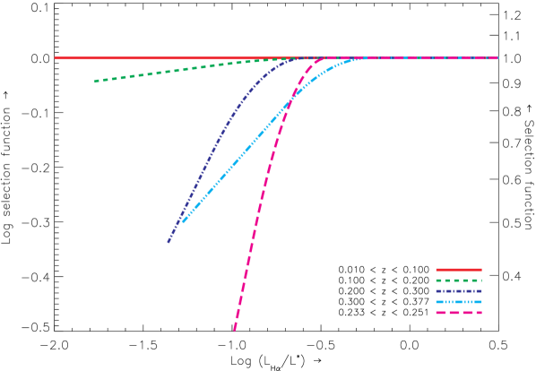
Figure 15: Logarithm of the selection function for each of the redshift bins sampled by SHELS as a function of with respect to $L^{*}$ at the respective redshift bin.

Given the input luminosity function, we can calculate the selection function for each redshift bin. We define the selection function as the ratio of the measured data points in Figure 10 and the intrinsic or “true” luminosity function. The selection function measures the effect of our $R\leq 20.3$ selection criterion. We show the selection functions in Figure 15.

At $z\sim 0.24$ we also consider the data of S08 These data should be complete over the luminosity range covered by SHELS. We thus assume the data from the narrowband survey as the intrinsic luminosity function and take the ratio between the S08 and the SHELS data as an estimate of the selection function (Figure 15; magenta long-dashed line). For consistency with the other redshift bins of SHELS we remove the OEW${}_{\mathrm{\ha+{\mbox{[{\sc N\,ii}]}}}}\geq 12$ Å constraint in this calculation (solid diamonds in Figure 9).

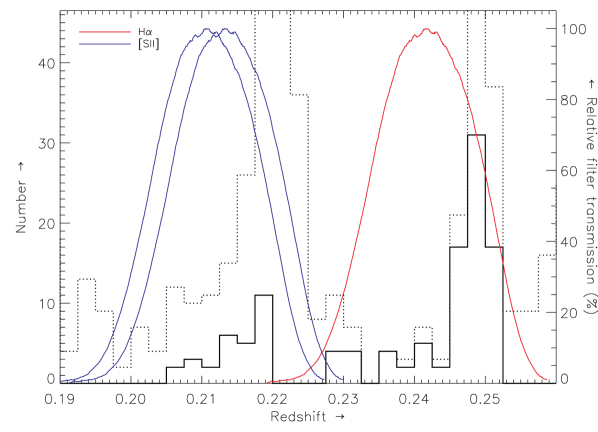
Figure 16: Redshifts from zCOSMOS DR2 of candidates of S08 (solid histograms) and all galaxies (dotted histogram), and the relative NB816 filter transmission curve for (red line) and both [S ii] lines (blue lines). Note the S08 galaxies within the [S ii] sensitive redshift range.

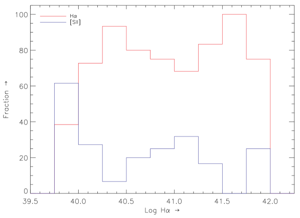
Figure 17: Fraction of candidates with a redshift from zCOSMOS DR2 corresponding to ($z\sim 0.24$; red histogram) or [S ii] ($z\sim 0.21$; blue histogram) as a function of luminosity calculated from the narrowband survey of S08.

The selection function computed at $z\sim 0.24$ using S08 should lie on top of the SHELS selection function at $0.200<z<0.300$, but it does not. Thus either SHELS underestimates–or S08 overestimates–the number of faint galaxies. Either the $R$-band magnitude vs. -luminosity relation between SHELS and S08 must be significantly different, or there is another selection effect not yet considered. Figure 6 rules out a different $R$- relation. This figure shows that the two surveys clearly overlap and do not have a significantly different $R$- relation.

A selection effect that removes some galaxies from the SHELS sample is the OEW${}_{\mathrm{\ha+{\mbox{[{\sc N\,ii}]}}}}\geq 12$ Å criterion. Figure 9 shows the effect of this criterion; it slightly increases the number of galaxies at the faint-end of the SHELS luminosity function. This bias is, however, insufficient to explain the differences in the SHELS- and S08-based selection functions.

The narrowband survey of S08 may overestimate the number of fainter galaxies. Even though consistent within the uncertainties, the faint-end slope of the combined luminosity function at $z\sim 0.24$ is somewhat steeper ($\alpha\sim-1.4$) than at our lowest redshift bin ($\alpha\sim-1.2$) causing a very steep selection function at $z\sim 0.24$.

We can determine the redshift of several narrowband-survey candidates of S08 using zCOSMOS DR2. Figure 16 shows the redshifts of the galaxies from S08 with confirmed redshifts near $z\sim 0.24$. Several galaxies have redshifts outside the wavelength range where the NB816 filter is sensitive to at $z\sim 0.24$ (red line). About 25 % of the candidates with spectroscopy are at a lower redshift $z\sim 0.21$. This redshift correspond to the wavelength range where the NB816 filter is sensitive to the [S ii] $\lambda\lambda$6733,6718 doublet (blue lines). These galaxies belong to an overdensity in the large-scale structure at $z\sim 0.22$ (dotted histogram in Figure 16 and solid histogram in Figure 8).

Figure 17 shows the fraction of galaxies with redshifts corresponding to [S ii] or as a function of the S08 luminosity. The figure suggests that the fraction of [S ii] galaxies increases towards fainter luminosities. This effect could produce an excess of faint galaxies in the S08 survey and thus could explain the difference in the selection functions implied by the SHELS simulations and the comparisons of SHELS and S08.

Color-color selections are sufficient to remove contaminating galaxies from the narrowband survey at higher redshifts. The contaminants include H$\beta$ and [O iii] at $z\sim 0.6-0.7$, [Oii] at $z\sim 1.2$ and Ly$\alpha$ at $z\sim 5.7$ for a narrowband survey at $\sim 8150$ Å (e.g. Fujita et al., 2003; Ly et al., 2007). However, it is impossible to distinguish galaxies from [S ii] galaxies by color (Westra & Jones, 2008). The contamination is survey dependent because it depends on the details of the large-scale structure. The S08 survey is a case where there is a peak in the redshift distribution exactly where the narrowband survey is sensitive to [S ii].

5.4 Volume dependence

There is a large spread in the parameters determined from different surveys around $z\sim 0.24$ (Figure 12) accompanied by very large uncertainties. All of these surveys (Fujita et al., 2003; Hippelein et al., 2003; Ly et al., 2007; Westra & Jones, 2008) use a single or multiple narrowband filters over $\sim 300-950\,\sq\arcmin$. S08 uses $5540\,\sq\arcmin$. Typical volumes are $0.5-1\times 10^{4}\,{\mathrm{Mpc^{3}}}$; S08 covers $3\times 10^{4}\,{\mathrm{Mpc^{3}}}$. The smaller volumes are not large enough to constrain the bright end of the luminosity function. We discussed S08 in detail in Section 4.

To examine the impact of small volumes, we split SHELS into 16 separate pieces to match the area ($\sim 0.25\,\sq\arcdeg$) of typical narrowband surveys that probe redshift $\sim 0.24$. Table 4 gives the median recovered parameters and the inter-quartile range.

For $\alpha=-1.20$ the recovered parameters are almost identical to those of the entire field. The inter-quartile range is large, even when compared to the uncertainties in Table 2. If we combine the 16 “surveys”, we would have to increase the uncertainties in Table 2 because of the smaller number of galaxies, i.e. an increase in shot-noise. This uncertainty easily explains the scatter of the parameters observed at $z\sim 0.24$. It underscores the need for large-volume surveys to constrain the bright end of the luminosity function.

To constrain $\alpha$ it is more important to have a deep survey and to span a large range of luminosities rather than to cover a large area. The data from Ly et al. (2007) demonstrate this point. As discussed in S08, the data-points from S08 and Ly et al. are quite similar at the fainter luminosities, both in slope and in amplitude. Thus, the survey area of Ly et al., i.e. $\sim 0.25\,\sq\arcdeg$, can be large enough to constrain $\alpha$, and $\alpha$ only. Their area (volume) is too small to determine the bright end of the luminosity function (see also S08, ) because they do not observe enough of the rare most-luminous galaxies.

To estimate the area required to constrain $L^{*}$ and $\phi^{*}$, we simulate many observed galaxies given a specific luminosity function at $0.233<z<0.251$ for different sized areas. We fit the parameters with fixed $\alpha=-1.20$. On average, the parameters are very well recovered. However, for the smaller areas the spread in the recovered parameters is large. We show the 1 $\sigma$ spread around the mean, the median, the inter-quartile range, and minimum and maximum values of the recovered values for each area in Figure 18.

Table 4: Median, upper and lower quartile range of Schechter parameters for 0.25 □° subsets using SHELS.

	fixed $\alpha$			unconstrained $\alpha$
redshift range	$\alpha$	$\log L^{*}$	$\log\phi^{*}$	$\alpha$	$\log L^{*}$	$\log\phi^{*}$
$0.010<z<0.100$	$-1.20$	$41.60_{-0.17}^{+0.23}$	$-2.79_{-0.13}^{+0.06}$	$-1.18_{-0.10}^{+0.19}$	$41.58_{-0.35}^{+0.23}$	$-2.76_{-0.34}^{+0.26}$
$0.100<z<0.200$	$-1.20$	$42.06_{-0.09}^{+0.10}$	$-2.96_{-0.13}^{+0.07}$	$-0.62_{-0.32}^{+0.10}$	$41.63_{-0.22}^{+0.18}$	$-2.57_{-0.05}^{+0.28}$
$0.200<z<0.300$	$-1.20$	$42.53_{-0.19}^{+0.13}$	$-3.28_{-0.12}^{+0.08}$	$-0.61_{-0.16}^{+0.15}$	$42.07_{-0.21}^{+0.21}$	$-2.75_{-0.07}^{+0.07}$
$0.300<z<0.377$	$-1.20$	$42.82_{-0.05}^{+0.04}$	$-3.56_{-0.09}^{+0.05}$	$-0.48_{-0.12}^{+0.17}$	$42.27_{-0.15}^{+0.04}$	$-2.96_{-0.24}^{+0.02}$
$0.233<z<0.251$	$-1.20$	$42.40_{-0.22}^{+0.22}$	$-3.28_{-0.09}^{+0.07}$	$-0.22_{-0.44}^{+0.21}$	$41.91_{-0.27}^{+0.11}$	$-2.79_{-0.63}^{+0.20}$

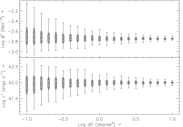
Figure 18: Box and whisker plot for the simulated surveys as a function of area. The surveys cover $0.233<z<0.251$ and have a limiting flux of $10^{-15.5}$ erg s^-1 cm^-2. The gray box indicates the 1 $\sigma$ around the mean, the dash indicates the median, the boxes indicates the inter-quartile range, and the whiskers indicate minimum and maximum values of recovered Schechter parameters (using the STY-method) from the simulations.

If we assume that 10 % is an acceptable uncertainty for a parameter ($\sim 0.04$ in dex), then the survey area required is $\sim 3\,\sq\arcdeg$. Surveys like Fujita et al. (2003), Ly et al. (2007) and Westra & Jones (2008) at $z\sim 0.24$ are thus not large enough to constrain the bright end of the luminosity function. S08 is a factor of two shy of this area; SHELS is larger.

Hence, combining the S08 and SHELS data (Section 4.2) is an excellent way to constrain the faint and bright end of the luminosity function simultaneously.

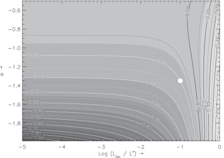
Figure 19: Logarithm of the total luminosity density evaluated at ($\log\frac{L_{\mathrm{lim}}}{L^{*}}$, $\alpha$) divided by the luminosity density at ($\log\frac{L_{\mathrm{lim}}}{L^{*}}$, $\alpha$) = (-1, -1.35) (white filled circle). The black lines indicate negative values.

6 Star formation density

We determine the star formation density ($\dot{\rho}$ in M_⊙ yr^-1 Mpc^-3) from the integrated luminosity density for each redshift range. We use the conversion from luminosity to star formation rate from Kennicutt (1998) for Case B recombination and $T_{e}=10^{4}$ K

$$\mathrm{SFR}=7.9\times 10^{-42}L_{\mathrm{\ha{}}},$$ (7)

where SFR in M_⊙ yr^-1 and $L_{\mathrm{\ha{}}}$ in erg s^-1. We determine the luminosity density for $L\geq L_{\mathrm{lim}}$ from the parameters of the Schechter function using

$$\mathcal{L}=\phi^{*}L^{*}\Gamma(\alpha+2,\frac{L_{\mathrm{lim}}}{L^{*}}),$$ (8)

where $\Gamma$ is the incomplete gamma function.

The choice $L_{\mathrm{lim}}=0$ affects the integrated luminosity density. Figure 19 shows the logarithm of the total luminosity density evaluated at ($\log\frac{L_{\mathrm{lim}}}{L^{*}}$, $\alpha$) divided by the luminosity density at ($\log\frac{L_{\mathrm{lim}}}{L^{*}}$, $\alpha$) = (-1, -1.35). We can thus determine the effect of using different limiting luminosities on the total luminosity density. For example, using $L_{\mathrm{lim}}=0$ for $\alpha=-1.35$ rather than $L_{\mathrm{lim}}=0.1L^{*}$ gives a difference of $10^{0.12-0.00}=1.31$, i.e. an increase of 30 %. These effects are obviously more severe for steeper values of $\alpha$. When comparing surveys of different depths, one needs to be careful about extrapolations of the luminosity function (Schechter function) to very low star formation rates, especially for steep $\alpha$.

Table 5: Star formation density.

		$\log\dot{\rho}$		$\log\dot{\rho}$ with $\log L_{\mathrm{lim}}=40$
redshift range	$\log L_{\mathrm{lim}}$	fixed $\alpha$	unconstrained $\alpha$	fixed $\alpha$	unconstrained $\alpha$
$0.010<z<0.100$	37.84	$-2.18\pm 0.10$	$-2.19\pm 0.17$	$-2.20\pm 0.10$	$-2.21\pm 0.17$
$0.100<z<0.200$	39.89	$-1.92\pm 0.09$	$-1.92\pm 0.12$	$-1.93\pm 0.09$	$-1.92\pm 0.12$
$0.200<z<0.300$	40.55	$-1.82\pm 0.05$	$-1.81\pm 0.10$	$-1.81\pm 0.05$	$-1.81\pm 0.10$
$0.300<z<0.377$	40.95	$-1.81\pm 0.03$	$-1.82\pm 0.08$	$-1.80\pm 0.03$	$-1.81\pm 0.08$
$0.233<z<0.251$				$\cdots$	$-1.86\pm 0.13$

Note. — We use the Schechter parameters determined for the pure star forming galaxies in Table 2. We calculate the uncertainties using standard uncertainty propagation for Eq. (8) and the uncertainties in Table 2. $\dot{\rho}$ is in M_⊙ yr^-1 Mpc^-3.

Table 5 lists the star formation densities and uncertainties for SHELS down to the luminosity limit of the appropriate redshift bin. We also show the star formation densities down to $\log L_{\mathrm{lim}}=40.00$ corresponding to a star formation rate of 0.079 M_⊙ yr^-1 for comparison with other surveys (Figure 20). We choose this value for all surveys because most surveys either reach this star formation rate, or the required extrapolation is modest. The solid symbols in Figure 20 represent surveys with star formation densities derived from the line; the open symbols come from either the [Oii] or [O iii] line. Figure 20 shows that the star formation density for other surveys at $0.200<z<0.300$ is consistent with the star formation density determined from the combined luminosity function of SHELS and S08.

Figure 20: Star formation density as a function of look-back time and redshift for SHELS (red, green, blue, and cyan large solid circles) compared with other surveys using the line (solid symbols), or either [Oii] or [O iii] lines (open symbols) as star formation indicator. We also indicate the combined SHELS and S08 point (solid large magenta circle). We calculate the star formation density using the Schechter parameters of each survey to a limiting star formation rate of 0.079 M_⊙ yr^-1 (corresponds to $L_{\ha}{}=10^{40}$ erg s^-1) to reduce the systematic uncertainty from extrapolation to $L=0$ erg s^-1.

Figure 20 also shows a clear increase in the star formation density with increasing redshift. However, our lowest redshift point ($0.010\leq z<0.100$) lies below surveys at similar redshifts. This underestimate occurs because our field was selected against low redshift clusters. This survey is thus an underdense region at low redshifts and the star formation density is probably correspondingly underestimated.

Because we use the integrated Schechter function to determine the star formation density, the arguments in Section 5.4 for the Schechter parameters $L^{*}$ and $\phi^{*}$, are valid for the star formation density. The median, upper and lower quartile range for the star formation density for 0.25 □° subsets are in Table 6. Again, the recovered star formation density of a 0.25 □° subset is almost identical to that of the entire field, but the standard deviation in the star formation density is very large (almost a factor of 2). The large uncertainty mainly results from the scatter in $L^{*}$ and $\phi^{*}$. Again, combined with the increased uncertainties resulting from increased shot-noise, the spread in star formation densities at narrow redshift slices can easily be explained by sampling a volume that is too small.

Table 6: Median, upper and lower quartile range of the star formation density for 0.25 □° subsets using SHELS.

	$\log\dot{\rho}$
redshift range	fixed $\alpha$	unconstrained $\alpha$
$0.010<z<0.100$	$-2.25_{-0.23}^{+0.12}$	$-2.30_{-0.22}^{+0.12}$
$0.100<z<0.200$	$-1.96_{-0.15}^{+0.13}$	$-1.97_{-0.15}^{+0.25}$
$0.200<z<0.300$	$-1.84_{-0.13}^{+0.16}$	$-1.85_{-0.13}^{+0.16}$
$0.300<z<0.377$	$-1.78_{-0.05}^{+0.03}$	$-1.82_{-0.19}^{+0.03}$
$0.233<z<0.251$	$-1.95_{-0.26}^{+0.23}$	$-1.96_{-0.26}^{+0.23}$

Note. — The values for the star formation density are integrated down to $\log L_{\mathrm{lim}}=40$.

7 Physical properties of star forming galaxies

7.1 Stellar population age

In star forming galaxies the emission originates from gas surrounding the young stars. The spectrum from an actively star forming galaxy is dominated by the light emitted by these young stars. Figure 21 shows $D_{n}{4000}$, the ratio of the continuum red- and bluewards of the $H+K$ break and an indicator of the age of the stellar population (Balogh et al., 1999; Bruzual, 1983), as a function of the luminosity for pure star forming galaxies. A low $D_{n}{4000}$ $D_{n}{4000}\lesssim 1.44$; D. F. Woods et al. 2010; in preparation indicates a young stellar population. The majority of the emitting galaxies contain a young stellar population.

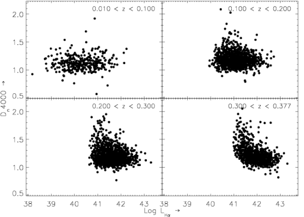
Figure 21: $D_{n}{4000}$ as a function of luminosity for each of the four redshift bins for pure star forming emitting galaxies.

7.2 Galaxy-galaxy interaction

Sobral et al. (2009) find that the fraction of mergers rises with increasing luminosity particularly around $L^{*}$. Some of the SHELS galaxies are quite luminous in indicating they are undergoing a starburst. Barton et al. (2000) find that a close pass of two galaxies can initiate a starburst. Following Sobral et al., we examine the SHELS data to look for evidence of the impact of interactions on the luminosity function. Thus, we focus on galaxies that may have (or may have had) a recent encounter with another galaxy. We determine whether each galaxy has an apparently nearby “neighbor”.

A galaxy has a neighbor when the velocity difference (corrected for redshift) between the two galaxies is $\leq 500\,{\mathrm{km\,s^{-1}}}$, and their projected separation is $\leq 100$ kpc. These values are a standard definition of galaxy pairs (e.g. Barton et al., 2000; Patton et al., 2000; Lin et al., 2004; Woods & Geller, 2007; Park & Choi, 2009). We include the somewhat deeper SHELS catalog to look for neighboring galaxies (see Section 2). This catalog contains spectra of galaxies with magnitudes $20.3<R<20.6$ where the spectroscopy is 52 % complete. The fraction of all our pure star forming galaxies that have a neighbor is 15.3 % (547 out of 3565).

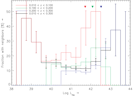
Figure 22: Fraction of pure star forming galaxies with one or more neighbors for each redshift bin (colored histograms) as a function of redshift and the fraction for $0.01<z<0.30$ (black thick histogram). Colored triangles indicate $L^{*}$ (determined with $\alpha=-1.20$) for each redshift range.

Figure 22 shows the fraction of galaxies with one or more neighbors as a function of luminosity for the lowest three redshift bins (colored histograms) and for the three redshift ranges combined (thick black histogram). The fraction is always a lower limit; deeper spectroscopy might reveal only more neighbors of a galaxy, never fewer.

It is striking that the fraction of galaxies with neighbors increases around $L^{*}$ (and for the lowest redshift bin towards the lowest luminosities). This result agrees with a rise in the fraction of mergers with increasing luminosity found by Sobral et al. (2009). The interesting question for galaxy evolution is whether the location of the increase determines $L^{*}$, or whether $L^{*}$ determines the location of the increase.

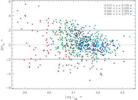
Figure 23: Magnitude difference between the galaxy and its neighbor as a function of luminosity for pure star forming emitting galaxies. The solid lines show $|\Delta m_{R}|=2$, the demarcation between major and minor interactions. Galaxies above the dotted line are fainter than their neighbor, galaxies below are more luminous.

To investigate this behavior further, we investigate the magnitude difference between the galaxy and its neighbor(s). Figure 23 shows the luminosity as a function of the magnitude difference $\Delta m_{R}=R_{\mathrm{galaxy}}-R_{\mathrm{neighbor}}$. We also indicate the demarcation between minor and major pairs, i.e. $|\Delta m|=2$ (e.g. Woods & Geller, 2007).

Luminous galaxies with neighbors tend to be mostly part of a major pair, and to a lesser extent the more luminous galaxy of a minor pair; faint galaxies with neighbors can be part of a major or minor pair. However, when faint galaxies are part of a minor pair, they tend to be the fainter (smaller) galaxy. The behavior in Figure 23 is consistent with the picture of interaction-induced star formation. The increase in the fraction around $L^{*}$ implies that galaxy-galaxy interactions are important for the increase of the luminosity in these galaxies.

8 Summary and conclusion

We use the Smithsonian Hectospec Lensing Survey (SHELS) to study emitting galaxies. SHELS is complete to $R_{\mathrm{tot}}=20.3$ over a large 4 □° area. This area yields a large enough volume to study the bright end of the luminosity function as a function of redshift.

We determine the flux and attenuation from the SHELS spectroscopy. We also identify galaxies that host AGNs or are composites.

We combine the strengths of two surveys, the breadth of SHELS (to constrain the bright-end of the luminosity function) and the depth of the narrowband survey of S08 (to determine the faint end slope of the luminosity function), to determine a well-constrained luminosity function at $z\sim 0.24$. A narrowband survey goes deep over a limited field of view to cover the faint end of the luminosity function. A broadband selected spectroscopic survey can easily cover a larger volume to probe the bright end of the luminosity function. The resulting Schechter parameters are consistent with S08 within their uncertainties.

We determine the luminosity function from SHELS for four redshift intervals over $0.010<z<0.377$. The lowest redshift interval ($0.010<z<0.100$) covers an atypical underdense region due to field selection. The characteristic luminosity $L^{*}$ increases as a function of redshift ($\Delta\log L^{*}=0.84$ over $0.100<z<0.377$).

The star formation density also increases with increasing redshift ($\Delta\log\dot{\rho}=0.11$ over $0.010<z<0.377$). The star formation rate from the combined luminosity function of SHELS and S08 is consistent with that of SHELS alone at $0.200<z<0.300$.

The fraction of galaxies with neighbors increases by a factor of $2-5$ around $L^{*}$ for the most luminous star forming galaxies at each redshift, similar to Sobral et al. (2009). The fraction appears to also increase towards fainter luminosity as a result of interactions in minor pairs. We conclude that triggered star formation is important for both the highest and lowest luminosity galaxies.

The future of surveys for star forming galaxies is a combination of a large-area spectroscopic survey combined with very deep narrowband imaging. However, the narrowband imaging requires extensive test spectroscopy because the impact of large-scale structure with respect to the filter response is unknown a priori. The combination of methods can constrain and remove the scatter in the star formation density as a function of redshift. The combination also allows a secure determination of the shape of the luminosity function over a large luminosity range.

Facilities: MMT (Hectospec)

References

- Adelman-McCarthy et al. (2008) Adelman-McCarthy, J. K., Agüeros, M. A., Allam, S. S., Allende Prieto, C., Anderson, K. S. J., Anderson, S. F., Annis, J., Bahcall, N. A., Bailer-Jones, C. A. L., Baldry, I. K., Barentine, J. C., Bassett, B. A., & et al. (SDSS collaboration). 2008, ApJS, 175, 297
- Baldwin et al. (1981) Baldwin, J. A., Phillips, M. M., & Terlevich, R. 1981, PASP, 93, 5
- Balogh et al. (1999) Balogh, M. L., Morris, S. L., Yee, H. K. C., Carlberg, R. G., & Ellingson, E. 1999, ApJ, 527, 54
- Barton et al. (2000) Barton, E. J., Geller, M. J., & Kenyon, S. J. 2000, ApJ, 530, 660
- Bell et al. (2005) Bell, E. F., Papovich, C., Wolf, C., Le Floc’h, E., Caldwell, J. A. R., Barden, M., Egami, E., McIntosh, D. H., Meisenheimer, K., Pérez-González, P. G., Rieke, G. H., Rieke, M. J., Rigby, J. R., & Rix, H.-W. 2005, ApJ, 625, 23
- Bertin & Arnouts (1996) Bertin, E. & Arnouts, S. 1996, A&AS, 117, 393
- Bruzual (1983) Bruzual, G. 1983, ApJ, 273, 105
- Bruzual & Charlot (2003) Bruzual, G. & Charlot, S. 2003, MNRAS, 344, 1000
- Calzetti (2001) Calzetti, D. 2001, PASP, 113, 1449
- Calzetti et al. (2000) Calzetti, D., Armus, L., Bohlin, R. C., Kinney, A. L., Koornneef, J., & Storchi-Bergmann, T. 2000, ApJ, 533, 682
- Capak et al. (2007) Capak, P., Aussel, H., Ajiki, M., McCracken, H. J., Mobasher, B., Scoville, N., Shopbell, P., Taniguchi, Y., Thompson, D., Tribiano, S., Sasaki, S., Blain, A. W., Brusa, M., Carilli, C., Comastri, A., Carollo, C. M., & et al. 2007, ApJS, 172, 99
- Cardelli et al. (1989) Cardelli, J. A., Clayton, G. C., & Mathis, J. S. 1989, ApJ, 345, 245
- Dale et al. (2008) Dale, D. A., Barlow, R. J., Cohen, S. A., Johnson, L. C., Kattner, S. A. M., Lamanna, C. A., Moore, C. A., Schuster, M. D., & Thatcher, J. W. 2008, AJ, 135, 1412
- Ellison et al. (2008) Ellison, S. L., Patton, D. R., Simard, L., & McConnachie, A. W. 2008, AJ, 135, 1877
- Fabricant et al. (2005) Fabricant, D., Fata, R., Roll, J., Hertz, E., Caldwell, N., Gauron, T., Geary, J., McLeod, B., Szentgyorgyi, A., Zajac, J., Kurtz, M., Barberis, J., Bergner, H., Brown, W., Conroy, M., Eng, R., Geller, M., Goddard, R., Honsa, M., Mueller, M., Mink, D., Ordway, M., Tokarz, S., Woods, D., Wyatt, W., Epps, H., & Dell’Antonio, I. 2005, PASP, 117, 1411
- Fabricant et al. (1998) Fabricant, D. G., Hertz, E. N., Szentgyorgyi, A. H., Fata, R. G., Roll, J. B., & Zajac, J. M. 1998, in Presented at the Society of Photo-Optical Instrumentation Engineers (SPIE) Conference, Vol. 3355, Society of Photo-Optical Instrumentation Engineers (SPIE) Conference Series, ed. S. D’Odorico, 285–296
- Fabricant et al. (2008) Fabricant, D. G., Kurtz, M. J., Geller, M. J., Caldwell, N., Woods, D., & Dell’Antonio, I. 2008, PASP, 120, 1222
- Fujita et al. (2003) Fujita, S. S., Ajiki, M., Shioya, Y., Nagao, T., Murayama, T., Taniguchi, Y., Umeda, K., Yamada, S., Yagi, M., Okamura, S., & Komiyama, Y. 2003, ApJ, 586, L115
- Gallego et al. (1995) Gallego, J., Zamorano, J., Aragon-Salamanca, A., & Rego, M. 1995, ApJ, 455, L1+
- Geach et al. (2008) Geach, J. E., Smail, I., Best, P. N., Kurk, J., Casali, M., Ivison, R. J., & Coppin, K. 2008, MNRAS, 388, 1473
- Geller et al. (2005) Geller, M. J., Dell’Antonio, I. P., Kurtz, M. J., Ramella, M., Fabricant, D. G., Caldwell, N., Tyson, J. A., & Wittman, D. 2005, ApJ, 635, L125
- Hippelein et al. (2003) Hippelein, H., Maier, C., Meisenheimer, K., Wolf, C., Fried, J. W., von Kuhlmann, B., Kümmel, M., Phleps, S., & Röser, H.-J. 2003, A&A, 402, 65
- Hopkins (2004) Hopkins, A. M. 2004, ApJ, 615, 209
- Hopkins & Beacom (2006) Hopkins, A. M. & Beacom, J. F. 2006, ApJ, 651, 142
- Hopkins et al. (2003) Hopkins, A. M., Miller, C. J., Nichol, R. C., Connolly, A. J., Bernardi, M., Gómez, P. L., Goto, T., Tremonti, C. A., Brinkmann, J., Ivezić, Ž., & Lamb, D. Q. 2003, ApJ, 599, 971
- Ilbert et al. (2005) Ilbert, O., Tresse, L., Zucca, E., Bardelli, S., Arnouts, S., Zamorani, G., Pozzetti, L., Bottini, D., Garilli, B., Le Brun, V., Le Fèvre, O., Maccagni, D., Picat, J.-P., Scaramella, R., Scodeggio, M., Vettolani, G., Zanichelli, A., Adami, C., Arnaboldi, M., Bolzonella, M., Cappi, A., Charlot, S., Contini, T., Foucaud, S., Franzetti, P., Gavignaud, I., Guzzo, L., Iovino, A., McCracken, H. J., Marano, B., Marinoni, C., Mathez, G., Mazure, A., Meneux, B., Merighi, R., Paltani, S., Pello, R., Pollo, A., Radovich, M., Bondi, M., Bongiorno, A., Busarello, G., Ciliegi, P., Lamareille, F., Mellier, Y., Merluzzi, P., Ripepi, V., & Rizzo, D. 2005, A&A, 439, 863
- Jones & Bland-Hawthorn (2001) Jones, D. H. & Bland-Hawthorn, J. 2001, ApJ, 550, 593
- Kauffmann et al. (2003) Kauffmann, G., Heckman, T. M., Tremonti, C., Brinchmann, J., Charlot, S., White, S. D. M., Ridgway, S. E., Brinkmann, J., Fukugita, M., Hall, P. B., Ivezić, Ž., Richards, G. T., & Schneider, D. P. 2003, MNRAS, 346, 1055
- Kennicutt (1998) Kennicutt, Jr., R. C. 1998, ARA&A, 36, 189
- Kewley et al. (2001) Kewley, L. J., Dopita, M. A., Sutherland, R. S., Heisler, C. A., & Trevena, J. 2001, ApJ, 556, 121
- Kewley et al. (2005) Kewley, L. J., Jansen, R. A., & Geller, M. J. 2005, PASP, 117, 227
- Kurtz & Mink (1998) Kurtz, M. J. & Mink, D. J. 1998, PASP, 110, 934
- Le Fèvre et al. (2000) Le Fèvre, O., Abraham, R., Lilly, S. J., Ellis, R. S., Brinchmann, J., Schade, D., Tresse, L., Colless, M., Crampton, D., Glazebrook, K., Hammer, F., & Broadhurst, T. 2000, MNRAS, 311, 565
- Li et al. (2008) Li, C., Kauffmann, G., Heckman, T. M., Jing, Y. P., & White, S. D. M. 2008, MNRAS, 385, 1903
- Lilly et al. (1996) Lilly, S. J., Le Fevre, O., Hammer, F., & Crampton, D. 1996, ApJ, 460, L1+
- Lilly et al. (2007) Lilly, S. J., Le Fèvre, O., Renzini, A., Zamorani, G., Scodeggio, M., Contini, T., Carollo, C. M., Hasinger, G., Kneib, J.-P., Iovino, A., Le Brun, V., Maier, C., Mainieri, V., Mignoli, M., Silverman, J., & et al. 2007, ApJS, 172, 70
- Lin et al. (2004) Lin, L., Koo, D. C., Willmer, C. N. A., Patton, D. R., Conselice, C. J., Yan, R., Coil, A. L., Cooper, M. C., Davis, M., Faber, S. M., Gerke, B. F., Guhathakurta, P., & Newman, J. A. 2004, ApJ, 617, L9
- Ly et al. (2007) Ly, C., Malkan, M. A., Kashikawa, N., Shimasaku, K., Doi, M., Nagao, T., Iye, M., Kodama, T., Morokuma, T., & Motohara, K. 2007, ApJ, 657, 738
- Madau et al. (1996) Madau, P., Ferguson, H. C., Dickinson, M. E., Giavalisco, M., Steidel, C. C., & Fruchter, A. 1996, MNRAS, 283, 1388
- Massarotti et al. (2001) Massarotti, M., Iovino, A., & Buzzoni, A. 2001, ApJ, 559, L105
- Mihos & Hernquist (1996) Mihos, J. C. & Hernquist, L. 1996, ApJ, 464, 641
- Mink et al. (2007) Mink, D. J., Wyatt, W. F., Caldwell, N., Conroy, M. A., Furesz, G., & Tokarz, S. P. 2007, in Astronomical Society of the Pacific Conference Series, Vol. 376, Astronomical Data Analysis Software and Systems XVI, ed. R. A. Shaw, F. Hill, & D. J. Bell, 249–+
- Moorwood et al. (2000) Moorwood, A. F. M., van der Werf, P. P., Cuby, J. G., & Oliva, E. 2000, A&A, 362, 9
- Morioka et al. (2008) Morioka, T., Nakajima, A., Taniguchi, Y., Shioya, Y., Murayama, T., & Sasaki, S. S. 2008, PASJ, 60, 1219
- Muller et al. (1998) Muller, G. P., Reed, R., Armandroff, T., Boroson, T. A., & Jacoby, G. H. 1998, in Presented at the Society of Photo-Optical Instrumentation Engineers (SPIE) Conference, Vol. 3355, Society of Photo-Optical Instrumentation Engineers (SPIE) Conference Series, ed. S. D’Odorico, 577–585
- Park & Choi (2009) Park, C. & Choi, Y.-Y. 2009, ApJ, 691, 1828
- Pascual et al. (2001) Pascual, S., Gallego, J., Aragón-Salamanca, A., & Zamorano, J. 2001, A&A, 379, 798
- Pascual et al. (2007) Pascual, S., Gallego, J., & Zamorano, J. 2007, PASP, 119, 30
- Patton et al. (2000) Patton, D. R., Carlberg, R. G., Marzke, R. O., Pritchet, C. J., da Costa, L. N., & Pellegrini, P. S. 2000, ApJ, 536, 153
- Pérez-González et al. (2003) Pérez-González, P. G., Zamorano, J., Gallego, J., Aragón-Salamanca, A., & Gil de Paz, A. 2003, ApJ, 591, 827
- Prescott et al. (2009) Prescott, M., Baldry, I. K., & James, P. A. 2009, MNRAS, 397, 90
- Roll et al. (1998) Roll, J. B., Fabricant, D. G., & McLeod, B. A. 1998, in Society of Photo-Optical Instrumentation Engineers (SPIE) Conference Series, Vol. 3355, Society of Photo-Optical Instrumentation Engineers (SPIE) Conference Series, ed. S. D’Odorico, 324–332
- Sandage et al. (1979) Sandage, A., Tammann, G. A., & Yahil, A. 1979, ApJ, 232, 352
- Schechter (1976) Schechter, P. 1976, ApJ, 203, 297
- Schmidt (1968) Schmidt, M. 1968, ApJ, 151, 393
- Shim et al. (2009) Shim, H., Colbert, J., Teplitz, H., Henry, A., Malkan, M., McCarthy, P., & Yan, L. 2009, ApJ, 696, 785
- Shioya et al. (2008) Shioya, Y., Taniguchi, Y., Sasaki, S. S., Nagao, T., Murayama, T., Takahashi, M. I., Ajiki, M., Ideue, Y., Mihara, S., Nakajima, A., Scoville, N. Z., Mobasher, B., Aussel, H., Giavalisco, M., Guzzo, L., Hasinger, G., Impey, C., Le Fèvre, O., Lilly, S., Renzini, A., Rich, M., Sanders, D. B., Schinnerer, E., Shopbell, P., Leauthaud, A., Kneib, J.-P., Rhodes, J., & Massey, R. 2008, ApJS, 175, 128
- Sobral et al. (2009) Sobral, D., Best, P. N., Geach, J. E., Smail, I., Kurk, J., Cirasuolo, M., Casali, M., Ivison, R. J., Coppin, K., & Dalton, G. B. 2009, MNRAS, 949
- Sullivan et al. (2000) Sullivan, M., Treyer, M. A., Ellis, R. S., Bridges, T. J., Milliard, B., & Donas, J. 2000, MNRAS, 312, 442
- Thompson et al. (1996) Thompson, D., Mannucci, F., & Beckwith, S. V. W. 1996, AJ, 112, 1794
- Tremonti et al. (2004) Tremonti, C. A., Heckman, T. M., Kauffmann, G., Brinchmann, J., Charlot, S., White, S. D. M., Seibert, M., Peng, E. W., Schlegel, D. J., Uomoto, A., Fukugita, M., & Brinkmann, J. 2004, ApJ, 613, 898
- Tresse & Maddox (1998) Tresse, L. & Maddox, S. J. 1998, ApJ, 495, 691
- Tresse et al. (2002) Tresse, L., Maddox, S. J., Le Fèvre, O., & Cuby, J.-G. 2002, MNRAS, 337, 369
- Treyer et al. (1998) Treyer, M. A., Ellis, R. S., Milliard, B., Donas, J., & Bridges, T. J. 1998, MNRAS, 300, 303
- Westra & Jones (2008) Westra, E. & Jones, D. H. 2008, MNRAS, 383, 339
- Wittman et al. (2006) Wittman, D., Dell’Antonio, I. P., Hughes, J. P., Margoniner, V. E., Tyson, J. A., Cohen, J. G., & Norman, D. 2006, ApJ, 643, 128
- Wittman et al. (2002) Wittman, D. M., Tyson, J. A., Dell’Antonio, I. P., Becker, A., Margoniner, V., Cohen, J. G., Norman, D., Loomba, D., Squires, G., Wilson, G., Stubbs, C. W., Hennawi, J., Spergel, D. N., Boeshaar, P., Clocchiatti, A., Hamuy, M., Bernstein, G., Gonzalez, A., Guhathakurta, P., Hu, W., Seljak, U., & Zaritsky, D. 2002, in Society of Photo-Optical Instrumentation Engineers (SPIE) Conference Series, Vol. 4836, Society of Photo-Optical Instrumentation Engineers (SPIE) Conference Series, ed. J. A. Tyson & S. Wolff, 73–82
- Woods & Geller (2007) Woods, D. F. & Geller, M. J. 2007, AJ, 134, 527
- Woods et al. (2006) Woods, D. F., Geller, M. J., & Barton, E. J. 2006, AJ, 132, 197