Active Galactic Nuclei in Groups and Clusters of Galaxies: Detection and Host Morphology

Abstract

The incidence and properties of Active Galactic Nuclei (AGN) in the field, groups, and clusters can provide new information about how these objects are triggered and fueled, similar to how these environments have been employed to study galaxy evolution. We have obtained new XMM-Newton observations of seven X-ray selected groups and poor clusters with $0.02<z<0.06$ for comparison with previous samples that mostly included rich clusters and optically-selected groups. Our final sample has ten groups and six clusters in this low-redshift range (split at a velocity dispersion of $\sigma=500$ $\textrm{km s}^{-1}$). We find that the X-ray selected AGN fraction increases from $f_{A}(L_{X}>10^{41};M_{R}<M_{R}^{*}+1)=0.047^{+0.023}_{-0.016}$ in clusters to $0.091^{+0.049}_{-0.034}$ for the groups (85% significance), or a factor of two, for AGN above an 0.3-8keV X-ray luminosity of $10^{41}$$\textrm{erg s}^{-1}$ hosted by galaxies more luminous than $M_{R}^{*}+1$. The trend is similar, although less significant, for a lower-luminosity host threshold of $M_{R}=-20$ mag. For many of the groups in the sample we have also identified AGN via standard emission-line diagnostics and find that these AGN are nearly disjoint from the X-ray selected AGN. Because there are substantial differences in the morphological mix of galaxies between groups and clusters, we have also measured the AGN fraction for early-type galaxies alone to determine if the differences are directly due to environment, or indirectly due to the change in the morphological mix. We find that the AGN fraction in early-type galaxies is also lower in clusters $f_{A,n>2.5}(L_{X}>10^{41};M_{R}<M_{R}^{*}+1)=0.048^{+0.028}_{-0.019}$ compared to $0.119^{+0.064}_{-0.044}$ for the groups (92% significance), a result consistent with the hypothesis that the change in AGN fraction is directly connected to environment.

1. Introduction

While it is clear that the Active Galactic Nuclei are powered by accretion onto supermassive black holes (SMBHs), and that this accretion requires both a source of fuel and a trigger to remove angular momentum from the fuel, the origin of the fuel and the trigger mechanism(s) remain poorly understood. For luminous QSOs, major mergers between gas-rich galaxies are considered the dominant mechanism and are the best, and perhaps only, candidate. Many studies have shown that a large fraction of these galaxies are morphologically disturbed, with close neighbors, tidal tails, multiple nuclei, or linked by luminous matter to other galaxies (Gehrens, Fried, Wehinger, & Wyckoff, 1984; Hutchings, Crampton, Campbell, 1984; Malkan, Margon, & Chanan, 1984; Smith et al., 1986). These results have motivated the hypothesis that lower-luminosity AGN in the local Universe are, like QSOs, triggered and fueled by galaxy mergers or at least interactions, even though there is no evidence to support the claim that mergers are the trigger for low-luminosity AGN (Fuentes-Williams & Stocke, 1988; Schmitt, 2001). If gas-rich mergers or interactions are the primary trigger for these lower-luminosity AGN, there should be higher AGN fractions in environments where galaxies have an abundant supply of gas and frequent interactions. While the cluster environment has very high number densities, the galaxies in the centers of rich clusters have less cold gas than those in less dense environments (e.g. Giovanelli & Haynes, 1985). In addition, the high pairwise velocity dispersions of cluster members may be too large to allow the formation of bound pairs inside the virial radius (e.g. Ghigna et al., 1998). In contrast, galaxies in the field have abundant supplies of cold gas, but the relatively low galaxy number density may counterbalance the abundance of fuel. Between these two extremes, the intermediate group environment could provide the ideal circumstances for the triggering and fueling of low-luminosity AGN in the nearby Universe, at least if mergers and interactions make a substantial contribution (although see Martini, 2004). Galaxies in groups have sufficiently modest velocity dispersions, numerous neighbors, and available cold gas to trigger and fuel AGN.

Many observations have shown that AGN are rarer in clusters when selected via emission-line diagnostics (Gisler, 1978; Dressler et al., 1985). Recent observations with the the Sloan Digital Sky Survey have shown this holds across a wide range in galaxy number density, specifically for the most luminous AGN (Miller et al., 2003; Kauffmann et al., 2004; Popesso & Biviano, 2006). These results have readily been explained with the argument outlined above, namely that insufficient cold gas reservoirs and high velocity dispersions discourage the triggering and fueling of AGN in the cluster environment. However, these same observations have indicated that the differences between environments fade for less luminous AGN, and additionally samples of lower-luminosity AGN may vary substantially depending on the selection technique employed. The differences in member morphology and physical environment between clusters and the field, as well as the relatively unbiased nature of X-ray observations, prompted Martini et al. (2006) to conduct a survey for X-ray AGN in nearby clusters. They found a factor of five higher AGN fraction than previous studies, where the AGN were identified to have X-ray luminosities $L_{X}\geq 10^{41}$ $\textrm{erg s}^{-1}$ in host galaxies more luminous than $M_{R}=-20$ mag. This dramatic increase was attributed to the greater sensitivity of X-ray observations to lower-luminosity AGN relative to visible-wavelength emission-line diagnostics (Baldwin, Phillips, & Terlevich, 1981) because the contrast between X-ray emission from AGN and other physical processes (low-mass X-ray binaries, hot gas, and star formation) is higher than in the case of the emission-line diagnostics.

To date only a small number of studies have attempted to extend work on X-ray selected AGN to the lower-velocity dispersion group environment. The first of these was a study of optically-selected groups at $z\sim 0.06$ by Shen et al. (2007). These authors only identified one AGN via X-ray selection out of 140 galaxies in eight groups, yet found five based on emission lines. More recently, Sivakoff et al. (2008) compared two, more massive groups and four clusters at similar redshifts and found a significantly higher X-ray selected AGN fraction in the groups compared to the clusters. One of the main goals of the present study is to dramatically improve on the small group sample in the Sivakoff et al. (2008) study, as well as to provide a larger sample of more massive groups than those in the Shen et al. (2007) study to better span the range of galaxy density from the field to clusters. While the groups in the Shen et al. (2007) sample are representative of those found in redshift surveys, they are otherwise a fairly heterogeneous sample. In contrast, the X-ray selection of this sample strongly suggests that these are all virialized systems. This local sample also provides a valuable benchmark for observations of the AGN fraction in groups and clusters at higher redshifts (e.g. Jeltema et al., 2007; Silverman et al., 2009; Martini, Sivakoff, & Mulchaey, 2009). For example, at $z=0.5-1$ Georgakakis et al. (2008) find a similar fraction of X-ray selected AGN in optically-selected groups as Shen et al. (2007) in the local universe.

Our other motivation is to investigate the role of galaxy morphology on the observed AGN fraction, as well as on the selection of AGN. Observations of many galaxies have shown that there is a strong correlation between the mass of the SMBH at the center of a given galaxy and the velocity dispersion or luminosity of the host galaxy’s spheroid component (Ferrarese & Merritt, 2000; Gebhardt et al., 2000; Marconi & Hunt, 2003). These relationships imply the coevolution of SMBHs and spheroids, and many authors have suggested that AGN may actively impact the evolution of the host galaxy by quenching star formation (Silk & Rees, 1998; Di Matteo, Springel, & Hernquist, 2005; Hopkins et al., 2005; Springel, Di Matteo, & Hernquist, 2005). Since AGN are a consequence of matter accreting onto the central SMBH, and the relation between SMBH mass and bulge properties implies a connection in their evolution, there may be a relation between the incidence of AGN and galaxy morphology. Observations by Ho et al. (1997) with the nearby Palomar Seyfert Survey, and more recent work with SDSS (Kauffmann et al., 2003), indicate that this is the case. These studies find that Seyferts are preferentially found in early-type spirals with a significant bulge. One potential interpretation of this result is that because early-type galaxies of a given mass will have larger SMBHs compared to late-type galaxies of the same mass, if their SMBHs both accrete at the same fixed fraction of the Eddington rate, then the early-type galaxy is more likely to be detected in a luminosity-limited sample.

This is important for comparing galaxy populations between groups, clusters, and the field because galaxy morphology is observed to be a strong function of local galaxy density (Dressler, 1980). Furthermore, many of the physical processes that are invoked to explain the relation between galaxy morphology and density may also have relevance for the available fuel supply for AGN. These include mergers and ram-pressure stripping via interactions with the hot ICM (Gunn & Gott, 1972; Quilis, Moore, & Bower, 2000), evaporation of the cold ISM by the host ICM (Cowie & Songaila, 1977), and starvation of new gas that would otherwise replenish the ISM (Larson et al., 1980; Balogh et al., 2000). There are thus correlations between morphology and the incidence of AGN, and between morphology and galaxy environment. It is therefore necessary to take morphology into account in order to determine if any variation in AGN fraction with environment is directly due to the environment itself, or indirectly due to the change in the mix of galaxy types with environment.

To disentangle the effects of morphology and environment we present new observations of rich groups and poor clusters selected from the NORAS sample of Böhringer et al. (2000). These observations and the X-ray AGN classification procedure are described in §2. In addition, we use spectroscopic data from SDSS to classify AGN based on emission-line diagnostics and compare these AGN to those selected via X-ray emission. We then combine these new data with previous work (Martini et al., 2006; Sivakoff et al., 2008) to study the incidence of AGN as a function of environment and morphology. The morphological classification is described in detail in §3, and the AGN fractions are presented in §4. The results, including a statistical analysis, are described in §5. The final section contains a summary of our main results. Throughout this paper we assume $H_{0}=70$ $\textrm{km s}^{-1}$ Mpc^-1.

2. Observations and Sample Selection

2.1. XMM-Newton Observations

Previous studies of X-ray AGN and environment have concentrated on rich clusters (Martini et al., 2006) and optically-selected groups (Shen et al., 2007; Georgakakis et al., 2008). X-ray detected groups represent the intermediate mass-scale between rich clusters and poor groups. To study the X-ray AGN population in X-ray detected groups, we observed a sample of seven low-redshift X-ray groups with the XMM-Newton telescope. The groups were selected from the NORAS catalog, which provides a large, uniform sample of X-ray bright groups and clusters found in the ROSAT All-Sky Survey (Böhringer et al., 2000). Our groups were selected based on the following three criteria: 1) X-ray luminosities between $3\times 10^{42}$ $\textrm{erg s}^{-1}$ and $3\times 10^{43}$ $\textrm{erg s}^{-1}$ in the 0.1-2.4 keV band. This luminosity range was chosen to be comparable to the luminosity range of the intermediate redshift X-ray groups in the sample of Mulchaey et al. (2006), potentially allowing a comparison of similar systems from redshift zero to $z\sim 0.5$; 2) Redshifts between 0.04 and 0.06. This redshift slice was chosen because it allows all of the groups to be studied out to approximately the virial radius in a single XMM-Newton pointing; 3) Spectroscopic coverage from the SDSS. SDSS spectroscopic coverage provides good membership information for each group. This last criterion also allows us to calculate an estimate of the AGN fraction based on standard emission-line diagnostics (see § 2.2.2 below) and to perform morphological fits of the surface brightness profiles of these objects from the SDSS imaging data (see § 3). The above selection criteria result in a sample of 14 X-ray luminous groups and poor clusters. From these 14 groups, we selected seven that span the X-ray luminosity range of interest.

The seven X-ray groups were observed by XMM-Newton between May 2007 and December 2007. The integration times varied from 12 to 40 ksec. All observations were obtained in full-frame mode with the thin optical blocking filter. The data were processed with version 7.0 of the XMMSAS software. For EMOS data we used only patterns 0–12 and apply the #XMMEA_EM flag filtering, while for EPN data we used patterns 0–4 and set the flag equal to zero. We eliminated periods of high background using the method described in Jeltema et al. (2006). This procedure involves filtering the data in several energy bands. We begin by applying a cut on the high energy ($>$10 keV) count rate of 0.35 counts s^-1 for EMOS data and 1.0 counts s^-1 for EPN data. We then applied a $3\sigma$ clipping to the source-free count rate in three energy bands. For this process, we used time bins of length 100 seconds. Time bins with rates more than $3\sigma$ from the mean are then removed until the mean is stable. Background flaring was very severe for one of the groups (RXCJ1225.2+3213) and resulted in no usable data. We therefore eliminated this group from our sample. For the remaining six groups, the final exposure times were in the range $\sim$ 10 to 23 ksec for the EMOS detectors. We note that we only include groups in our XMM-Newton analysis for which we can reach a lower limit of $L_{X}=10^{41}$ $\textrm{erg s}^{-1}$ at a radius of 13^′.

To better constrain the AGN population in groups, we supplemented our sample with additional groups that have XMM-Newton observations available from the archive. These groups were also selected from the NORAS catalog in the same X-ray luminosity range described above (criterion 1). We also required that these groups had spectroscopic coverage in the SDSS (criterion 3). However, we did not require these groups to be in the redshift range 0.04 to 0.06. To insure that a significant fraction of the group members were within the XMM-Newton field of view we only considered groups that had XMM-Newton coverage out to a radius of at least 250 kpc. Using these revised criteria, we added another five groups to our sample, bringing the total number of NORAS-selected groups to eleven. The XMM-Newton observations for these additional groups were reduced following the same method described above. The final exposure times for all five of these groups is at least 10 ksec in the EMOS detectors.

Membership was determined with the method described in Mulchaey et al. (2006) and largely based on the available SDSS spectroscopy in the fields on these groups and clusters. We start with all galaxies located within a projected distance of 1 Mpc from the center with a recessional velocity within $\pm 3000$ $\textrm{km s}^{-1}$ of the mean velocity. We then calculate the velocity dispersion of the system using the biweight estimator (Beers et al., 1990). Objects with velocities greater than three times the velocity dispersion away from the mean are then removed from the sample and a new mean and dispersion are calculated. This process is continued until no further objects are removed. Note that although we have estimated the global properties from galaxies located within 1 Mpc of the center, our AGN analysis is restricted to the smaller radii probed by the XMM-Newton data.

Table 1Groups and Clusters

Group/Cluster Name	Alternate Name	RA	Dec	Redshift	— Members —		$\sigma_{v}$	Data Sources
					$N$	$N^{*}$	[km s-1]
(1)	(2)	(3)	(4)	(5)	(6)	(7)	(8)	(9)
A85		00:41:50.4	-09:18:11	0.0554	109	53	$993^{+85}_{-85}$	1,3
A644		08:17:25.6	-07:30:45	0.0701	75	40	$952^{+382}_{-382}$	2,3
A3128		03:30:43.8	-52:31:30	0.0595	67	28	$906^{+74}_{-74}$	2,3
RXCJ0110.0+1358		01:10:05.5	+13:58:49	0.0581	30	15	$745^{+74}_{-64}$	1,4
RXCJ0746.6+3100	ZwCl0743.5+3110	07:46:37.3	+31:00:49	0.0579	23	16	$719^{+97}_{-59}$	1,4
RXCJ1022.0+3830		10:22:04.7	+38:30:43	0.0544	36	18	$710^{+77}_{-54}$	1,4
A3125		03:27:17.9	-53:29:37	0.0616	20	15	$475^{+94}_{-94}$	2,3
A89B		00:42:54.6	-09:13:50	0.0770	22	12	$474^{+155}_{-155}$	1,3
RXCJ0844.9+4258		08:44:56.7	+42:58:54	0.0550	13	9	$343^{+75}_{-34}$	1,4
RXCJ1002.6+3241	ZwCl0959.6+3257	10:02:38.6	+32:41:58	0.0505	33	9	$454^{+58}_{-39}$	1,4
RXCJ1122.2+6712		11:22:14.5	+67:12:46	0.0553	22	8	$223^{+27}_{-23}$	1,4
RXCJ1204.4+0154	MKW4	12:04:25.6	+01:54:04	0.0203	12	7	$495^{+59}_{-45}$	1,4
RXCJ1223.1+1037	NGC4325	12:23:06.5	+10:37:26	0.0255	4	2	$334^{+51}_{-32}$	1,4
RXCJ1324.1+1358	NGC5129	13:24:11.9	+13:58:45	0.0233	6	3	$303^{+47}_{-29}$	1,4
RXCJ1440.6+0328	MKW8	14:40:38.2	+03:28:25	0.0269	15	9	$449^{+41}_{-30}$	1,4
RXCJ1604.9+2355	AWM4	16:04:57.0	+23:55:14	0.0321	9	3	$423^{+58}_{-36}$	1,4

Note. — Properties of all groups and clusters employed in this study. Columns are: (1) Name in the original NORAS catalog or from Sivakoff et al. (2008); (2) Alternate name from the literature, if any; (3 and 4) RA and DEC of the X-ray center; (5) redshift; (6 and 7) number of members more luminous than $M_{R}=-20$ and $M_{R}^{*}+1$, respectively; (8) velocity dispersion; (9) references for data. References are 1: SDSS DR6 images and spectroscopy (Adelman-McCarthy et al., 2008); 2: 2.5m du Pont Telescope (Martini et al., 2006); 3: Chandra X-ray Observatory (Martini et al., 2006; Sivakoff et al., 2008); 4: XMM-Newton, this work.

We supplemented these observations of NORAS groups and clusters with other, primarily rich clusters, with redshifts in the range $0.05<z<0.08$. The details of these observations are presented in Martini et al. (2006) and Sivakoff et al. (2008). Briefly, these studies are based on X-ray observations with Chandra and ground-based images and spectroscopy from Las Campanas Observatory in Chile. Further details are provided in these two papers. Our final list of groups and clusters is provided in Table 1, along with the source of the data for each group or cluster. Throughout this study we separate groups and clusters based on whether the velocity dispersion is greater or less than 500$\textrm{km s}^{-1}$. Some of the implications of this choice are discussed in §4.1. The division of the groups and clusters in Table 1 reflect this threshold value.

2.2. AGN Classification

While very luminous AGN can be unambiguously identified in almost any energy band, AGN become progressively more challenging to identify at lower luminosities when their emission may be equal or even substantially less than that of their host galaxy. These lower-luminosity AGN are important to identify to maximize the sample of AGN for demographic studies. It is also important to understand the completeness of the AGN selection to connect to other studies. At a minimum, the completeness should be expressed in terms of luminosity in some band, although results are more readily compared with theory if they can be expressed in terms of bolometric luminosity or accretion rate relative to the mass of the black hole. Here we identify AGN via their X-ray luminosity, which is estimated to represent on order 10% of the bolometric luminosity with small scatter (e.g. Elvis et al., 1994; Marconi et al., 2004) and consequently it is a reasonable proxy. X-rays also have the advantage that they are relatively less sensitive to the effects of extinction. For the low-luminosity AGN we consider here, other physical processes can also produce comparable X-ray emission from galaxies, so in the first subsection below we describe our AGN classification technique in detail. The main alternative method to identify AGN is via visible-wavelength emission-line ratios and we compare our X-ray classification to this other method in the following subsection ($\S$ 2.2.2).

In addition to careful selection of AGN via either method, characterization of how the AGN population varies across different environments can be reasonably performed with a measurement of the fraction of all galaxies of a given morphology that host AGN. In previous studies (e.g. Martini et al., 2002, 2006) the AGN fraction was defined as the fraction of galaxies with absolute magnitude $M_{R}\leq-20$ mag (Vega) that host AGN with a broad-band [0.3-8keV] X-ray luminosity of $L_{X}\geq 10^{41}$ $\textrm{erg s}^{-1}$. To identify a comparable host luminosity range with the NORAS sample, we converted the SDSS extinction-corrected, $r-$band magnitudes (on the AB system) to Bessel $R-$band (on the Vega system) and applied a mean $k-$correction for each group. For both of these steps we employed the software tools described by Blanton & Roweis (2007). We also adopt the evolving absolute magnitude threshold of $M_{R}\leq M_{R}^{*}(z)+1$ introduced by Martini, Sivakoff, & Mulchaey (2009) to compare samples across a wide range in redshift, where $M_{R}^{*}(z)=M_{R}^{*}(0)-z$, and $M_{R}^{*}(z=0)=-21.92$. For the present sample the evolution term ($z$) is negligible and the main result is a second threshold approximately one magnitude more luminous than the previous magnitude cut. This higher threshold is useful because the AGN fraction increases when a higher luminosity threshold is used (Sivakoff et al., 2008).

2.2.1 X-ray Classification

We created images in the 0.5 to 8 keV band for each detector using the flare-cleaned event files spatially binned to give 2^′′ pixels. The images for the three detectors were combined to form a final image using the SAS task emosaic. To identify X-ray sources, we ran the task ewavelet on the merged image with a detection threshold of 5$\sigma$. The X-ray detections were then compared to the known members to determine matches. We restrict this analysis to objects within 13^′ of the field center. All sources within 2^′′ of the center of a known member are considered matches; we are motivated to use this search radius by the 1$\sigma$ positional uncertainty of XMM of $1-2^{\prime\prime}$ (Watson et al., 2009). As is typical of nearby X-ray groups and poor clusters, the diffuse X-ray emission is centered on or near the brightest galaxy in most cases (Mulchaey & Zabludoff, 1998; Osmond & Ponman, 2004). This makes searching for an AGN component difficult for the central galaxies and we have therefore excluded these objects from our analysis. This is also the case with the analysis of the richer clusters in our sample (Martini et al., 2006).

For each member detected by XMM, we extract a surface brightness profile to determine the extent of the X-ray emission. We extracted source spectra in circular regions extending to where the surface brightness profile reaches the background level. Local background spectra were extracted from annular regions immediately surrounding the source. Using a local background of this type includes any additional background from the diffuse intragroup medium at the location of the source. Response files (RMFs and ARFs) were constructed for the location of the source using the SAS tasks rmfgen and arfgen, respectively. Source spectra were binned to have 25 counts bin^-1.

All spectral fitting was performed using XSPEC (version 12.3). As noted briefly above, the four main physical processes that can produce substantial ($L_{X}>10^{40}$ $\textrm{erg s}^{-1}$) broad-band (0.3–8keV) X-ray emission from galaxies are AGN, a population of low-mass X-ray binaries (LMXBs), thermal emission from hot gas, and emission from the high-mass X-ray binaries (HMXBs) and supernova remnants associated with substantial recent star formation. We classify an X-ray source as an AGN if the observed X-ray luminosity exceeds that expected from these other physical processes that can produce X-ray emission. Our basic procedure is described in Sivakoff et al. (2008), which improves on the earlier procedure employed by Martini et al. (2006). Briefly, we use relations between X-ray luminosity, $K-$band luminosity, and star formation rate to determine the expected contribution from LMXBs (cf.  Kim & Fabbiano, 2004), star formation (cf.  Grimm, Gilfanov, & Sunyaev, 2003), and halos of hot gas (cf.  Sun et al., 2007) and classify a galaxy as an AGN if the X-ray luminosity exceeds the expected contribution from these other sources of emission.

Because these XMM observations often have sufficient counts for spectral fits, we fit two spectral models to better classify AGN when the data are sufficient. These models are a single power-law component to represent the combined emission of the LMXBs and any AGN component and a thermal component to represent any emission from hot gas. We then estimate the X-ray binary emission expected from the $K-$band luminosity of the galaxy and consider any excess emission from the power-law component to be due to an AGN. In all our fits the neutral hydrogen column density is fixed at the Galactic value given in Kalberla et al. (2005). We also fix the power-law index ($\Gamma$) to 1.7. For the thermal component, we use the MEKAL model in XSPEC with the abundance fixed at 0.8 solar. We simultaneously fit the spectra from all three EPIC detectors. For galaxies with at least several hundred counts, it is usually possible to constrain both the thermal and powerlaw components. In some cases, only one component is required to produce an adequate fit (i.e. the normalization of the second component is consistent with zero). For galaxies with a small number of counts, it is not possible to distinguish between the possible spectral models. For these objects, we have estimated the X-ray luminosity assuming a power-law model alone. The resulting luminosities of the power-law and thermal components for each galaxy are given in Table 2. We note that if a thermal model is assumed for the cases where the spectral model cannot be determined, the resulting luminosities would be lower by a factor of approximately two.

Table 2X-ray Detected Group Members

Galaxy	MR	LK	Model	LXpowerlaw	LXthermal	Class
				1040 erg s-1	1040 erg s-1
				(0.3-8.0 keV)	(0.3-8.0 keV)
(1)	(2)	(3)	(4)	(5)	(6)	(7)
2MASXJ07463295+3101213	-22.6	11.42	Po1	18.6${}^{+10.3}_{-9.1}$	-	AGN
2MASXJ07462331+3101183	-22.2	11.36	Po1	10.3${}^{+7.4}_{-5.5}$	-	inactive
2MASXJ08445063+4302479∗	-23.1	11.67	Po	24.1${}^{+9.0}_{-8.5}$	-	AGN
2MASXJ10230356+3838176	-21.0	10.70	Po1	72.2${}^{+31.4}_{-30.8}$	-	AGN
2MASXJ10223745+3834447	-23.2	11.69	Po+ Th	104.9${}^{+27.8}_{-39.1}$	33.0${}^{+48.5}_{-8.5}$	AGN
2MASXJ10220069+3829145	-21.9	11.03	Po1	23.2${}^{+8.8}_{-8.2}$	-	AGN
2MASXJ11231618+6706308	-22.1	11.22	Po1	16.6${}^{+10.7}_{-7.8}$	-	AGN
2MASXJ11221610+6711219	-21.5	10.96	Po	14.0${}^{+7.3}_{-6.5}$	-	AGN
2MASXJ11223691+6710171n	-21.6	11.03	Po1	8.5${}^{+13.9}_{-4.2}$	-	AGN
SDSSJ112333.56+671109.9	-20.1	-	Po+ Th	40.7${}^{+15.1}_{-12.0}$	14.9${}^{+18.1}_{-4.5}$	AGN
2MASXJ12043806+0147156	-22.5	11.33	Po+ Th	7.2${}^{+3.7}_{-2.0}$	2.8${}^{+4.3}_{-1.2}$	inactive
2MASXJ12225772+1032540	-21.3	11.08	Po+ Th	2.6${}^{+2.1}_{-1.1}$	1.4${}^{+2.7}_{-0.4}$	inactive
2MASXJ13242889+1405332	-22.3	11.43	Po	10.0${}^{+1.8}_{-1.8}$	-	inactive
2MASXJ14403793+0322375	-22.3	11.38	Po	6.1${}^{+1.7}_{-1.9}$	-	inactive

Note. — X-ray measurements and classifications. Columns are: (1) Galaxy name; (2) Host galaxy $R-$band absolute magnitude; (3) Total $K-$band luminosity from 2MASS (for SDSSJ112333.56+671109.9 $K=14$ mag was assumed based on the colors of other group members); (4) Model fit to the X-ray data where Po is a power-law fit, Th is a thermal model, and Po¹ indicates a power-law was assumed (see $\S$ 2.2.1); (5) X-ray luminosity of the power law component; (6) X-ray luminosity of the thermal component; (7) classification of the galaxy as either an AGN or as inactive. $L_{X,po}$ and $L_{X,th}$ are in units of $10^{40}$ $\textrm{erg s}^{-1}$ and are broad-band (0.3-8keV) measurements. The ^∗ superscript in Column 1 denotes the single galaxy in the NORAS sample that is classified as an AGN based both on its X-ray properties and its emission lines. The ⁿ superscript refers to an AGN below our $L_{X}=10^{41}$ $\textrm{erg s}^{-1}$ limit and thus not included in the sample statistics.

The additional spectral information available for many of these sources better constrains the nature of the X-ray emission. Specifically, eight of the 14 X-ray sources associated with members have sufficient signal-to-noise ratio to determine if the X-ray emission was best-fit by a power-law model, thermal model, or both. This improves the classification over, e.g. Sivakoff et al. (2008) as we can then compare the luminosity of the best-fit power-law model to just the expected emission from LMXBs, HMXBs, and an AGN component, and exclude the thermal model because of its different spectrum. The top panel of Figure 1 shows the broad-band X-ray luminosity of the best-fit power-law component for all of these eight galaxies compared to the $K-$band luminosity. Note that whereas in Sivakoff et al. (2008) we used the 2MASS $K_{20}$ magnitude, here we employ the $K_{total}$ magnitude as this is a better match to the aperture used for the X-ray photometry. The figure also shows the expected relationship between X-ray luminosity and $K-$band luminosity for LMXBs from Kim & Fabbiano (2004), where the thicker line is the relation and the thinner lines are $\pm 1\sigma$ uncertainties. Four of the eight X-ray sources fall on the LMXB relation and we classify these galaxies as inactive (see Table 2). The remaining four are at least $2\sigma$ more X-ray luminous than would be expected from LMXBs alone and we therefore classify these galaxies as X-ray AGN. We note that these classifications are the same as we would have assigned based on our previous approach with an $L_{X}=10^{41}$ $\textrm{erg s}^{-1}$ threshold (Martini et al., 2006; Sivakoff et al., 2008).

Figure 1.— The broad-band X-ray luminosity $L_{X,B}$ vs. the near-IR luminosity, $L_{K_{s},\mathrm{tot}}$ for the galaxies displayed in Table 2. The top panel shows the broad-band X-ray luminosity $L_{X,B}$ of the best-fit power-law component for all of these eight galaxies compared to the $K-$band luminosity. Here we compare to the expected relation for LMXBs (dotted line) from Kim & Fabbiano (2004) and classify four of eight galaxies as X-ray AGN (stars). The bottom panel shows the relation for sources with insufficient counts for spectral modeling. Here we assume a $\Gamma=1.7$ power law and compare with the sum (solid line) of the LMXB relation and a thermal model (dashed line) from Sun et al. (2007). Five of the sources are classified as AGN, although one is below $10^{41}$ $\textrm{erg s}^{-1}$ and is not included in the statistical analysis. In both panels the thicker line is the relation and the thinner lines are $\pm 1\sigma$ uncertainties. Other galaxies are classified as inactive (filled circles, see Table 2).

The other six galaxies had sufficiently faint X-ray emission that we were unable to accurately model their X-ray spectra. In these cases we followed the procedure used by Sivakoff et al. (2008) and assumed a $\Gamma=1.7$ model and measured the X-ray luminosity of that model. These six sources are shown in the bottom panel of Figure 1 along with the same LMXB relation shown in the top panel, a relation between $L_{X}$ and $L_{K}$ for thermal emission from hot gas adapted from Sun et al. (2007), and the sum of these two relations, where again the inactive galaxy relation is represented by the thicker line and the $\pm 1\sigma$ uncertainties are represented by thinner lines. The hot gas relation is modified from that presented by Sun et al. (2007) because their measurements were in the soft band (0.5-2keV) and ours are broad-band (0.3-8keV) measurements. We therefore multiplied their X-ray luminosity by the flux ratio of a $kT=0.7$keV thermal bremsstrahlung model in the broad band and soft band. In practice none of the sources in the lower panel are sufficiently luminous in the $K-$band that we expect a substantial thermal component. Five of the six sources are above the relation by at least $2\sigma$ and we classify these galaxies as X-ray AGN, although one of these is not included in our statistical analysis because it has $L_{X}<10^{41}$ $\textrm{erg s}^{-1}$. We also note that none of these 14 galaxies appears to have sufficient star formation to contribute significantly to the X-ray luminosity. To check this we estimated star formation rates for each galaxy from the H$\alpha$ flux (e.g. Kennicutt, 1998; Brinchmann et al., 2004) and then calculated the expected X-ray luminosity from Grimm, Gilfanov, & Sunyaev (2003). In all cases the estimated X-ray luminosity due to star formation was at least an order of magnitude below the observed luminosity. For the five groups and clusters in common with Sivakoff et al. (2008) we retain the same AGN classifications presented in that paper.

2.2.2 Emission-Line Classification

The traditional technique to identify low-luminosity AGN in emission-line galaxies is through use of line ratios such as $[\mathrm{OIII}]\lambda 5007/\mathrm{H}\beta$ and $[\mathrm{NII}]\lambda 6584/\mathrm{H}\alpha$ on a “BPT Diagram” (Baldwin, Phillips, & Terlevich, 1981). We have measurements of these four emission lines for most (349) of the galaxies in the sample from the NORAS catalog from the MPA-JHU galaxy catalog for the SDSS Data Release 7. We use the emission-line measurements and errors calculated by the MPA-JHU group, which have been corrected for stellar absorption, and then calculate emission line ratios. If the line flux measurements for $[\mathrm{NII}]\lambda 6584/\mathrm{H}\alpha$ are larger than 3 times the error associated with the measurements, we keep the data for analysis. We are less conservative for the $[\mathrm{OIII}]\lambda 5007/\mathrm{H}\beta$ ratio because galaxies with precise $[\mathrm{NII}]\lambda 6584/\mathrm{H}\alpha$ measurements can be unambiguously identified as AGN even if the $[\mathrm{OIII}]\lambda 5007/\mathrm{H}\beta$ measurements are less certain (e.g. Shen et al., 2007). In addition, edge-on galaxies might obscure the bluer $[\mathrm{OIII}]$ and $\mathrm{H}\beta$ lines, leading to a misclassification. We hope to keep these possibly obscured but still unambiguous AGN in our sample by being less stringent with our condition on the $[\mathrm{OIII}]\lambda 5007/\mathrm{H}\beta$ measurement errors.

Figure 2.— A BPT Diagram (Baldwin, Phillips, & Terlevich, 1981) for all galaxies with sufficiently bright emission-lines in our NORAS sample. Inactive galaxies (open circles) are separated based on whether $M_{R}>-20$ mag (small open circles), $-20\geq M_{R}\geq M_{R}^{*}+1$ (medium open circles), or have $M_{R}\leq M_{R}^{*}+1$ (large open circles). The X-ray AGN (filled circles) and BPT AGN (stars) are similarly scaled based on host galaxy luminosity and all AGN have error bars. Galaxies are classified as BPT AGN if they fall above the Kewley et al. (2001) criterion (dot-dashed line). The criterion of Kauffmann et al. (2003) is also shown (dashed line).

Of the 349 galaxies in the MPA-JHU galaxy catalog, 116 have sufficiently bright spectral lines to place on the BPT Diagram shown in Figure 2. This figure illustrates the values of $[\mathrm{NII}]\lambda 6584/\mathrm{H}\alpha$ and $[\mathrm{OIII}]\lambda 5007/\mathrm{H}\beta$ for these 116 galaxies. We identify galaxies as “BPT AGN” if these two line ratios place them above the threshold suggested by Kewley et al. (2001) as the maximum limit that could be produced by extreme starburst activity. This is a very conservative limit and many confirmed AGN do not meet this criterion. For reference, we also show the less conservative threshold of Kauffmann et al. (2003). Of the 116 galaxies with sufficient emission-line detections to fall on this diagram, 14 were identified as BPT AGN. A total of 199 out of the 349 galaxies with SDSS spectra also have $M_{R}\leq-20$ mag, so the BPT AGN fraction for this sample is $14/199=0.070^{+0.024}_{-0.019}$ (all BPT AGN have $M_{R}\leq-20$ mag). For comparison, six of these 199 galaxies or $\sim 3$% were identified as X-ray AGN (note that not all X-ray AGN had sufficient spectral-line data). It is also striking that only one galaxy is classified as both an X-ray AGN and a BPT AGN. The samples are nearly disjoint. Further information about the galaxies identified as BPT AGN is provided in Table 3.

Table 3BPT AGN

Galaxy	MR	log($[\mathrm{OIII}]\lambda 5007/\mathrm{H}\beta$)	log($[\mathrm{NII}]\lambda 6584/\mathrm{H}\alpha$)
(1)	(2)	(3)	(4)
2MASXJ01095902+1358155	-20.8	0.182 $\pm$ 0.090	0.140 $\pm$ 0.166
SDSSJ010957.88+140320.1	-20.4	-0.032 $\pm$ 0.099	0.362 $\pm$ 0.292
SDSSJ011021.57+135421.4	-20.2	0.180 $\pm$ 0.119	0.501 $\pm$ 0.230
2MASXJ07462331+3101183	-22.2	0.164 $\pm$ 0.049	0.285 $\pm$ 0.082
2MASXJ07470054+3058205	-21.7	0.129 $\pm$ 0.050	0.207 $\pm$ 0.170
2MASXJ08445063+4302479 ∗	-23.1	0.032 $\pm$ 0.084	0.061 $\pm$ 0.078
SDSSJ100311.10+323511.3	-20.2	0.304 $\pm$ 0.062	0.362 $\pm$ 0.361
2MASXJ10213991+3831195	-21.5	-0.038 $\pm$ 0.119	0.278 $\pm$ 0.128
2MASXJ11223691+6710171 (VIIZw392)	-22.4	0.168 $\pm$ 0.020	0.005 $\pm$ 0.046
SDSSJ112425.38+671940.0	-20.3	0.115 $\pm$ 0.045	0.281 $\pm$ 0.092
2MASXJ12041899+015054 (CGCG013-058)	-21.2	0.129 $\pm$ 0.072	0.064 $\pm$ 0.146
2MASXJ12230667+1037170 (NGC4325)	-22.5	0.151 $\pm$ 0.027	-0.251 $\pm$ 0.171
2MASXJ12225772+1032540	-21.3	-0.082 $\pm$ 0.152	0.343 $\pm$ 0.106
2MASXJ13241000+1358351 (NGC5129)	-23.1	0.162 $\pm$ 0.084	0.086 $\pm$ 0.120

Note. — Galaxies identified as AGN on the BPT Diagram (Baldwin, Phillips, & Terlevich, 1981) shown in Figure 2. Columns are: (1) The name (alternate name) of the galaxy; (2) $M_{R}$; (3) calculated value of log $[\mathrm{OIII}]\lambda 5007/\mathrm{H}\beta$ from the MPA-JHU database; (4) calculated value of log $[\mathrm{NII}]\lambda 6584/\mathrm{H}\alpha$ from the MPA-JHU database. The ^∗ superscript in Column 1 denotes the only galaxy that is classified as an AGN based both on its X-ray properties and its visible-wavelength emission lines.

3. Morphological Analysis

Though galaxy morphology has been used extensively to study galaxy evolution, until recently this property was determined by eye. This process, though largely repeatable, lacks quantitative robustness and is a protracted process for large numbers of objects. The alternative—measuring morphology in an automated fashion—is not simple to implement. Only in the last decade, with the development of large-format, linear detectors and substantial computational resources, has it become commonplace to classify galaxies using quantitative and repeatable techniques. Datasets consisting of large numbers of galaxies have made visual inspection intractable as a method for determining morphology (although there have been novel approaches for morphological identification via visual inspection; see Lintott et al., 2008), while abundant computational resources have made large-scale, quantitative analyses more feasible.

Various methods to ascertain morphology quantitatively exist in the literature (Conselice, Bershady, & Jangren, 2000; Simard, 2002; Goto et al., 2003; Lotz et al., 2004), and we chose to use the galaxy fitting code GALFIT (Peng et al., 2002) to measure the morphological properties for galaxies in our sample. One of our main motivations for the choice of GALFIT was the work of Haeussler et al. (2007), who compared GALFIT to GIM2D (Simard, 2002) and concluded that GALFIT has advantages in its ability to simultaneously fit neighboring galaxies in a crowded field and benefits from a dramatic increase in execution speed. GALFIT is designed to extract structural components from galaxies by fitting two-dimensional light profiles with an arbitrary number of parametric functions that are suitable for describing the surface brightness distribution of galaxies. Although the code was authored to fit subtle structures of well-resolved galaxies with many-component models simultaneously, it is also effective at handling large numbers of galaxies imaged at lower resolution by fitting their surface brightness profiles with relatively simple models. We utilize the latter capability in our analysis. GALFIT takes as input a simple text file and is very customizable, allowing easy extension via a wrapper script. A final advantage is that GALFIT can use a variety of analytic functions singly or simultaneously, including the Sérsic profile. In the next subsections we describe the fitting procedure in more detail, including how we parametrize galaxy morphology, and present the results of our fits of the X-ray and BPT AGN. We fit models to all of the galaxies in our sample that have imaging data.

3.1. Model Fits

We have adopted two parameters to quantify galaxy morphology: the value of the Sérsic index $n$ and the bulge-to-total flux ratio $B/T$. The Sérsic profile is defined to be:

$$\Sigma(r)=\Sigma_{e}\mathrm{exp}\left[-\kappa\left(\left(\frac{r}{r_{e}}\right)^{1/n}-1\right)\right],$$ (1)

where $\Sigma_{e}$ is the surface brightness (flux per unit area) at the effective radius $r_{e}$, $r_{e}$ is the half-light radius, and the eponymous index $n$ characterizes the shape of the light profile. The parameter $\kappa$ is set by the constraint that $r_{e}$ is the half-light radius. The Sérsic index $n$ has been commonly used to separate early-type and late-type galaxies in the literature. Studies based on SDSS imaging data find that $n=2.5$ is a reasonable point to distinguish these two types (e.g. Bell et al., 2004a; McIntosh et al., 2005) and we too adopt $n\geq 2.5$ to identify early-type galaxies.

The bulge-to-total flux ratio is measured from a classic bulge-disk decomposition. Here we fit a bulge component with a de Vaucouleurs (1948) $r^{1/4}$ profile and a disk component with an exponential surface brightness profile. The fraction of the total flux in the bulge component relative to the total (bulge + disk) flux then provides the ratio $B/T$. Throughout this work we will primarily rely on the Sérsic index to classify galaxies, but we will use the $B/T$ as a consistency check on our results. Note also that $n=4$ is equivalent to the $r^{1/4}$ profile and $n=1$ is equivalent to an exponential disk profile.

When available we also compared our calculated morphological parameters to the SDSS fracDeV parameter, which is calculated by the SDSS pipeline and serves as another quantitative measure of galaxy morphology. The fracDeV parameter is very similar to our bulge-to-total flux decomposition. It is obtained by fitting the surface brightness profile of a galaxy with exponential and de Vaucouleurs components and then keeping the fractional contribution of the latter. Bernardi et al. (2005) identified fracDeV $>0.8$ to identify early-type galaxies.

As noted above, GALFIT accepts an input text file that specifies the initial conditions for models and other options and parameters related to the fit. GALFIT can accommodate as many independent models as the user desires, limited only by computational resources. It is also possible to simultaneously fit adjacent or blended objects in addition to the target to remove potential contamination and obtain a more robust fit. GALFIT convolves the model with a point spread function (PSF) supplied by the user, subtracts the convolved model from the input image, and computes the reduced chi squared, $\chi^{2}_{\nu}$:

$$\chi^{2}_{\nu}=\frac{1}{N_{\mathrm{dof}}}\sum_{x=1}^{nx}\sum_{y=1}^{ny}\frac{\left(\mathrm{flux}_{x,y}-\mathrm{model}_{x,y}\right)^{2}}{\sigma_{x,y}^{2}},$$ (2)

where $N_{\mathrm{dof}}$ is the number of degrees of freedom in the model, flux and model are the pixel values of the original image and analytic model, respectively, and $\sigma_{x,y}^{2}$ is the error in each pixel. GALFIT minimizes $\chi^{2}_{\nu}$ using a Levenberg-Marquardt algorithm, a downhill-gradient type algorithm suited for searching large parameter spaces quickly. Additional and optional input includes a bad pixel map specifying which pixels should be excluded from the $\chi^{2}_{\nu}$ calculation (i.e. masked out) and initial guesses for the many free parameters, including the astrometric and morphological quantities of the target.

GALFIT is useful in its extensibility and we took advantage of this by creating a wrapper script in Python and an algorithm to fit many target objects with little to no user interaction. The results are comparable to a human user fine tuning GALFIT input parameters until an ideal fit is obtained. The input to this process is a list of astrometric coordinates of targets and the FITS images in which these targets are imaged. For each target the script determines if it lies within the boundaries of a given image and obtains initial morphological parameters (e.g. a measure of the galaxy’s radius, magnitude, ellipticity, object position, and position angle) with SExtractor (Bertin & Arnouts, 1996). At this stage we retain information about all detected objects within some arbitrary number (found using trial and error) of effective radii from the target. The fitting region supplied to GALFIT is determined in a similar way. Based on the parameters of the objects in the field of view, we either add the pixels associated with the object to the bad pixel file, masking them out and removing them from the $\chi^{2}_{\nu}$ calculation and fitting procedure, or fit the object in addition to the target. This discriminatory algorithm compares object brightness to the target brightness (e.g. an object very much dimmer than the target will likely be masked out rather than fit) and the distance from the target (e.g. an object separated by many target galaxy-radii will likely be masked out rather than fit). In this way we only fit additional objects if they are likely to contaminate the fit of our target, and thus its morphological properties. Fitting a superfluous number of objects is computationally wasteful and complicates finding a unique minimum in $\chi^{2}_{\nu}$ space.

Our wrapper script generates a GALFIT input file for both a single component Sérsic profile fit and a two component Sérsic profile $+$ Exponential Disk fit. Several iterations of this dual method fitting occur if the resultant $\chi^{2}_{\nu}$ values for the two parameterizations differ by more than a small amount, with the previous fit parameters used for subsequent iterations, to insure that the solution obtained is not the result of the minimization algorithm getting lost in a local minimum. This propensity to get lost in a local minimum and the question of the uniqueness of a multi-component solution in large parameters spaces is an issue for algorithms like GALFIT, and Peng et al. (2002) addresses this question in depth (see their $\S$ 3.3).

Another requirement for GALFIT is an estimate of the PSF shape. These were created manually for each image by approximating them with a Gaussian generated with the standard gauss task in IRAF. Effective radii of the PSFs were estimated by examining several stars in each image. We determined that small variations in the radius of the PSF negligibly affected the parameters of the model, confirming the robustness of this approximate method of PSF creation.

When completed, the wrapper saves: 1) a postage stamp sized image of the original galaxy (i.e. a cropped section of the wide-field FITS image where the target fills the frame); 2) an image of the same size that displays the model generated by GALFIT convolved with the user-defined PSF; 3) a residual image: the original data less the convolved model. This third image should, if the model is perfect, show a scene identical to the input image, with the exception that the region of sky previously occupied by the target galaxy should be indistinguishable from noise (although somewhat increased noise due to the contribution of the subtracted object). Unsurprisingly, this ideal case is rare (though not nonexistent). These three images are saved for each fit technique (single and two-fit methods) for quick visual inspection. We also retain the fit log files generated by GALFIT, FITS images that contain the GALFIT models generated by the algorithm, and a text file with the relevant morphological parameters and object information for later use. The script that automates these tasks works for an arbitrarily large set of input targets.

3.2. Fit Results

The three-image results for all of the X-ray AGN are shown in Figure 3, while the results for the BPT AGN are shown in Figure 4. The model parameters associated with all of these fits are listed in Tables 4 and 5. Only one object falls in both samples and consequently appears in both figures and tables. While these figures demonstrate our results on AGN, described further below in §4.2, they also are fairly representative of our morphological fits to the inactive group and cluster galaxies.

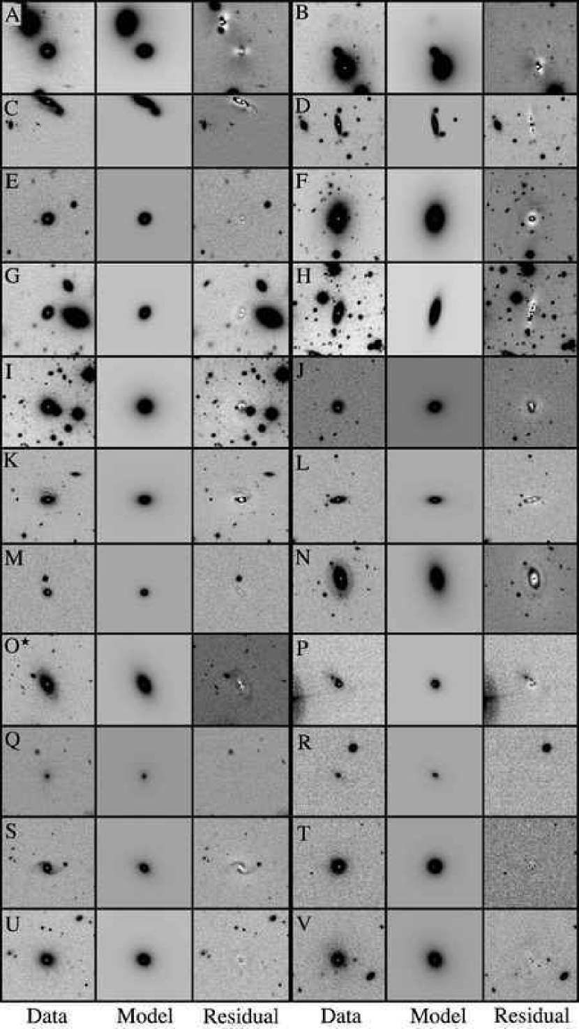
Figure 3.— Data, GALFIT models, and residuals of all the X-ray AGN for our entire sample. For details of the AGN identification see §2.2.1, Martini et al. (2006), and Sivakoff et al. (2008). The morphological parameters associated with these fits are listed in Table 4. The star symbol, next to Panel O, denotes the only galaxy in our sample identified as both a BPT AGN and an X-ray AGN. This object is also in Panel F in Figure 4.

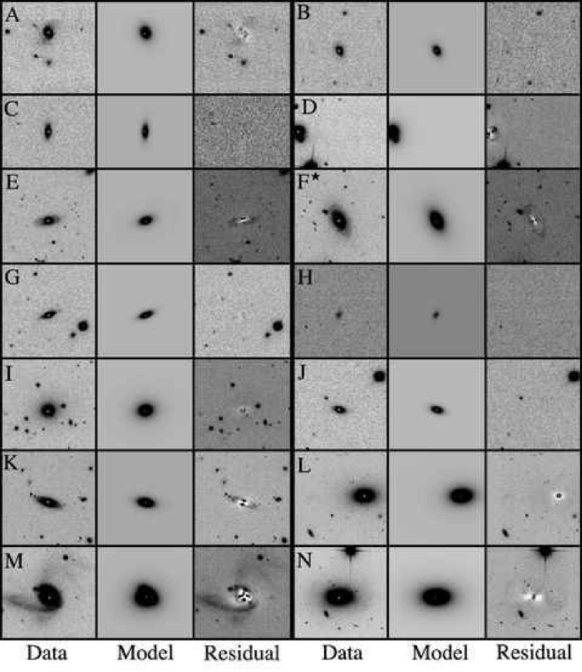
Figure 4.— Data, GALFIT models, and residuals of all the BPT AGN for our entire sample. For details of AGN identification see $\S$ 2.2.2. The morphological parameters associated with these fits are listed in Table 5. The star symbol, next to Panel F, denotes the only galaxy in our sample identified as both a BPT AGN and an X-ray AGN. This object is also in Panel O in Figure 3.

Table 4Fit Properties from Figure 3 — X-ray AGN

Panel	Cluster/Group	Object Name	Sérsic Index	$\chi^{2}_{\nu}$	fbulge / ftotal	$\chi^{2}_{\nu}$
(1)	(2)	(3)	(4)	(5)	(6)	(7)
A	A3125	J032723.4-532535.5	3.18	1.965	0.930	1.875
B	A3125	J032725.3-532506.6	2.27	1.635	0.768	1.638
C	A3125	J032705.1-532140.9	2.63	1.739	0.724	1.630
D	A3128	J033039.2-523205.7	1.24	1.300	0.109	1.236
E	A3128	J032941.4-522935.7	1.36	1.182	0.335	1.178
F	A3128	J033051.0-523031.2	4.53	1.528	0.964	1.652
G	A3128	J033017.3-523408.9	1.75	1.585	0.458	1.576
H	A644	J081748.1-073731.7	2.16	9.746	0.575	7.099
I	A644	J081739.5-073309.0	12.0	10.58	0.371	7.762
J	A85	J004311.6-093816.1	3.06	1.583	0.400	1.568
K	A85	J004130.3-091545.9	3.57	1.712	0.085	1.606
L	A89B	J004314.1-092145.2	2.89	1.538	0.545	1.532
M	RXCJ1122.2+6712	SDSSJ12333.56+671109.9	1.56	1.498	0.053	1.495
N	RXCJ0746.6+3100	2MASXJ07463295+3101213	4.28	2.044	1.000	2.038
O∗	RXCJ0844.9+4258	2MASXJ08445063+4302479 (CGCG208-041)	4.59	1.551	0.812	1.552
P	RXCJ1022.0+3830	2MASXJ10220069+3829145	2.37	6.604	0.808	6.556
Q	RXCJ1022.0+3830	2MASXJ10223745+3834447 (NGC 3219)	3.49	6.268	0.851	6.268
R	RXCJ1022.0+3830	2MASXJ10230356+3838176	9.38	6.672	0.534	6.672
S	RXCJ1122.2+6712	2MASXJ11221610+6711219	6.88	1.625	0.355	1.587
Tn	RXCJ1122.2+6712	2MASXJ11223691+6710171 (VIIZw394)	3.35	1.550	0.894	1.547
U	RXCJ1122.2+6712	2MASXJ11231618+6706308	4.60	1.520	1.000	1.524
V	A89B	J004300.63-091346.4	5.97	1.544	0.999	1.569

Note. — GALFIT output parameters from fits to all X-ray AGN. The ^∗ superscript in Column 1 identifies the only galaxy in our sample that is classified as both a BPT AGN and an X-ray AGN. This object is Object F in Table 5. The ⁿ superscript refers to an AGN below our $L_{X}=10^{41}$ $\textrm{erg s}^{-1}$ limit.

Table 5Fit Properties from Figure 4 — BPT AGN

Panel	Cluster/Group	Object Name	Sérsic Index	$\chi^{2}_{\nu}$	fbulge / ftotal	$\chi^{2}_{\nu}$
(1)	(2)	(3)	(4)	(5)	(6)	(7)
A	RXCJ0110.0+1358	2MASXJ01095902+1358155	2.99	1.625	0.932	1.648
B	RXCJ0110.0+1358	SDSSJ010957.88+140320.1	2.20	1.567	0.398	1.564
C	RXCJ0110.0+1358	SDSSJ011021.57+135421.4	1.96	1.523	0.562	1.524
D	RXCJ0746.6+3100	2MASXJ07462331+3101183	2.55	2.221	0.509	2.112
E	RXCJ0746.6+3100	2MASXJ07470054+3058205	2.96	1.604	0.613	1.582
F∗	RXCJ0844.9+4258	2MASXJ08445063+4302479 (CGCG208-041)	4.59	1.551	0.812	1.552
G	RXCJ1002.6+3241	SDSSJ100311.10+323511.3	1.51	1.424	0.472	1.427
H	RXCJ1022.0+3830	2MASXJ10213991+3831195	1.13	6.372	0.022	6.372
I	RXCJ1122.2+6712	2MASXJ11221537+671318 (VIIZw392)	4.86	1.595	0.667	1.582
J	RXCJ1122.2+6712	SDSSJ112425.38+671940.0	1.69	1.531	0.509	1.532
K	RXCJ1204.4+0154	2MASXJ12041899+015054 (CGCG013-058)	2.17	1.798	0.726	1.747
L	RXCJ1223.1+1037	2MASXJ12230667+1037170 (NGC4325)	2.42	1.627	0.884	1.579
M	RXCJ1223.1+1037	2MASXJ12225772+1032540	3.96	2.313	0.977	2.316
N	RXCJ1324.1+1358	2MASXJ13241000+1358351 (NGC5129)	4.22	1.805	0.792	1.762

Note. — GALFIT output parameters from fits to all BPT AGN. The ^∗ superscript in Column 1 identifies the only galaxy in our sample that is classified as both a BPT AGN and an X-ray AGN. This object is Object O in Table 4.

One common challenge to most fits is crowding. Figure 3, Panel H shows a galaxy in the cluster A644 where many neighbors have been removed by subtraction and only the target was fit with GALFIT. Our algorithm determined that all neighbors were sufficiently far or faint enough that they did not interfere with the fitting procedure. To obtain a low value of $\chi^{2}_{\nu}$, the pixels from these other objects in the field of view were simply masked out. Figure 3, Panel D depicts a similar but slightly more challenging case. Here the target is blended with a bright, nearby object. In this case multiple objects are fit to obtain a reasonable model for the target. As before, objects yet further away are simply masked out. Panels A & B present additional examples of this case. A final case is illustrated by Figure 4, Panel M. In this case the model is simply inadequate because the galaxy’s morphology is more complicated than our simple models. This galaxy appears to be both blended with other objects and morphologically disturbed.

Figure 5.— Bulge-to-total flux ratio versus Sérsic index for all of the groups and clusters in our sample. Points are as in Figure 2 for X-ray AGN (filled circles), BPT AGN (stars), and inactive galaxies (open circles). This plot includes all the galaxies successfully fit with GALFIT, though the BPT AGN are only selected from the subsample with adequate Sloan spectra. The dashed line is drawn at $n=2.5$.

The algorithm used by GALFIT is optimized for speed and is searching a very large parameter space; consequently the probability of getting lost in a local minimum is non-negligible. Though it is difficult to be certain that this has not happened for most cases, we employ several techniques to guard against this possibility. First, we run GALFIT on each target several times and update the initial fit parameters if the resultant $\chi^{2}_{\nu}$ differs by more than several percent between two runs. Second, we fit two distinct sets of models to each galaxy in separate runs: the Sérsic index in a single component fit and the bulge-to-total flux ratio in a two component model fit. These quantities are correlated for most galaxies (see Figure 5) and we carefully reexamine egregious outliers. Finally, we save output images, as shown in Figures 3 and 4, and inspect these to identify poor fits.

Stubborn objects that are not well fit by our procedure persist, though they are relatively few. As noted above, GALFIT was originally developed by Peng et al. (2002) with the purpose of decomposing the complex structure of well resolved galaxies. We instead use it to do simple one- or, at most, two-model fits. For our typical resolution and galaxy size this is not a problem. However, some of the galaxies in our images are so well resolved that a simple Sérsic profile or de Vaucouleurs bulge plus exponential disk fit is insufficient to adequately describe the morphology. Structures such as bars or prominent spiral arms are sometimes fit rather than the more averaged profile of the galaxy that may have resulted from a less well-resolved image of the same object. Also, we occasionally find objects that are blended or coincident with the target and cannot be simultaneously with the target, such as the example of Panel M of Figure 4 mentioned above. In general, blending is a particularly challenging problem if SExtractor fails to find the blended object as a distinct source.

Figure 6.— Sérsic index versus SDSS fracDeV parameter for all of the galaxies with SDSS coverage. Points are as in Figure 2 for X-ray AGN (filled circles), BPT AGN (stars), and inactive galaxies (open circles). The solid line is a linear fit and the dashed lines are drawn at $n=2.5$, where we separate early and late-type galaxies, and the interception of the fit line with $n=2.5$, at fracDeV $=0.66$.

In addition to comparison of the correlation between the Sérsic index and the bulge-to-total flux ratio shown in Figure 5, we also compare to the SDSS fracDeV parameter when available. We find that these two parameters do not correlate well, while our Sérsic index measurements do correlate with the fracDeV parameter, as shown in Figure 6, although the scatter is significant. One source of scatter is that the fracDeV parameter saturates while we still measure a substantial range of Sérsic index. We fit a line to this relation, although excluded points with fracDeV $=1$, and found that fracDeV $=0.66$ corresponds to $n=2.5$. This is reasonably consistent with the value of fracDeV $=0.8$ used in the literature to identify early-type galaxies (e.g. Bernardi et al., 2005). As for Figure  5, we visually inspected all outliers on this figure to check the goodness of fit.

Table 6Morphological Results

Cluster / Group	— $N_{\mathrm{fit}}$ —		$f_{n>2.5}$	—— $N_{\mathrm{total}}$ ——			— $N_{\mathrm{fit}^{*}}$ —		$f_{n>2.5}^{*}$	—— $N_{\mathrm{total}}^{*}$ ——
	$All$	$n>2.5$		$Raw$	$Corr$	$n>2.5$	$All$	$n>2.5$		$Raw$	$Corr$	$n>2.5$
(1)	(2)	(3)	(4)	(5)	(6)	(7)	(8)	(9)	(10)	(11)	(12)	(13)
A85	104	76	0.731${}^{+0.094}_{-0.084}$	109	109	80	49	41	0.837${}^{+0.152}_{-0.130}$	53	53	44
A644	15	7	0.467${}^{+0.278}_{-0.231}$	19	75	35	6	5	0.833${}^{+0.167}_{-0.360}$	40	40	33
A3128	54	21	0.389${}^{+0.105}_{-0.084}$	67	67	26	25	15	0.600${}^{+0.198}_{-0.153}$	28	28	17
RXCJ0110.0+1358	30	19	0.633${}^{+0.181}_{-0.144}$	30	30	19	15	12	0.800${}^{+0.200}_{-0.228}$	15	15	12
RXCJ0746.6+3100	23	17	0.739${}^{+0.226}_{-0.177}$	23	23	17	16	14	0.875${}^{+0.125}_{-0.231}$	16	16	14
RXCJ1022.0+3830	36	11	0.306${}^{+0.123}_{-0.091}$	36	36	11	18	6	0.333${}^{+0.199}_{-0.132}$	18	18	6
All Clusters	262	151	0.576${}^{+0.051}_{-0.047}$	284	340	188	129	93	0.721${}^{+0.083}_{-0.075}$	170	170	126
A3125	18	10	0.556${}^{+0.237}_{-0.173}$	20	28	16	11	10	0.909${}^{+0.091}_{-0.283}$	15	15	14
A89B	14	7	0.500${}^{+0.269}_{-0.184}$	22	22	11	7	5	0.714${}^{+0.286}_{-0.308}$	12	12	9
RXCJ0844.9+4258	13	10	0.769${}^{+0.231}_{-0.239}$	13	13	10	9	8	0.889${}^{+0.111}_{-0.308}$	9	9	8
RXCJ1002.6+3241	33	16	0.485${}^{+0.154}_{-0.120}$	33	33	16	9	6	0.667${}^{+0.333}_{-0.264}$	9	9	6
RXCJ1122.2+6712	22	8	0.364${}^{+0.179}_{-0.126}$	22	22	8	8	5	0.625${}^{+0.375}_{-0.270}$	8	8	5
RXCJ1204.4+0154	12	9	0.750${}^{+0.250}_{-0.245}$	12	12	9	7	6	0.857${}^{+0.143}_{-0.340}$	7	7	6
RXCJ1223.1+1037	4	2	0.500${}^{+0.500}_{-0.323}$	4	4	2	2	1	0.500${}^{+0.500}_{-0.414}$	2	2	1
RXCJ1324.1+1358	6	2	0.333${}^{+0.440}_{-0.215}$	6	6	2	3	2	0.667${}^{+0.333}_{-0.431}$	3	3	2
RXCJ1440.6+0328	15	7	0.467${}^{+0.251}_{-0.172}$	15	15	7	9	5	0.556${}^{+0.376}_{-0.240}$	9	9	5
RXCJ1604.9+2355	9	7	0.778${}^{+0.222}_{-0.287}$	9	9	7	3	3	1.000${}^{+0.000}_{-0.544}$	3	3	3
All Groups	146	78	0.534${}^{+0.068}_{-0.060}$	156	164	88	68	51	0.750${}^{+0.120}_{-0.105}$	77	77	59

Note. — Morphological and demographic information for our two samples. Columns are: (1) Cluster or group name; (2) Number of objects successfully fit by GALFIT with $M_{R}\leq-20$ mag; (3) The number objects from column 2 with $n>2.5$; (4) Fraction of objects from column 2 with $n>2.5$; (5) Number of confirmed objects with $M_{R}\leq-20$ mag; (6) Number of objects after a completeness correction, if any; (7) Number of objects in the sample with $n>2.5$, corrected for completeness, if applicable; (8-13) Same as columns 2–7, but with the brighter magnitude cut ($M_{R}=M_{R}^{*}$ + 1). The errorbars on the fractions are all single-sided, one-sigma confidence intervals (Gehrels, 1986).

We performed this morphological analysis on all of the confirmed member galaxies and additional groups and clusters from (Sivakoff et al., 2008). We used these data to identify all of the early-type galaxies in each group and cluster with $M_{R}\leq-20$ mag and $M_{R}\leq M_{R}^{*}+1$ and calculate the early-type galaxy fraction. These results are presented in Table 6, which includes the total number of galaxies and the number successfully fit. Typically these numbers agree, except for rare instances when some galaxies were not fit successfully.

4. AGN Fractions

The next step of our analysis is to combine the AGN classifications from §2.2 and the morphology fits from §3 to measure the AGN fraction as a function of environment and determine if there is any variation with host galaxy morphology. This analysis is described in the first subsection below. In addition, in §2.2 above we demonstrated that the X-ray AGN and BPT AGN were nearly disjoint populations. In the following subsection we compare the morphologies of these two populations. Throughout we calculate AGN fractions for absolute magnitude limits of $M_{R}\leq-20$ mag and $M_{R}\leq M_{R}^{*}+1$ and in all cases the AGN fraction is defined to be the number of AGN divided by the total number galaxies above a given absolute magnitude limit. All errorbars are derived from Poisson and binomial statistics and are single-sided, $1\sigma$ confidence intervals (Gehrels, 1986).

4.1. X-ray AGN

Table 7 provides the number of X-ray identified AGN in each group or cluster, the X-ray AGN fraction, and the X-ray AGN fraction with early-type host galaxies. These results are also illustrated graphically in Figures 7 and 8, although groups and clusters with no AGN are not shown for clarity. In both figures the top panel shows the results for the absolute magnitude threshold of $M_{R}\leq-20$ mag and the bottom panel for $M_{R}\leq M_{R}^{*}+1$. These figures indicate that the AGN fraction is smaller in environments characterized by a higher velocity dispersion.

Table 7X-ray AGN Fractions

Cluster/Group	$N_{X,fit,n>2.5}$	$N_{X,fit}$	$f_{X}$	$f_{X,n>2.5}$	$N_{X,fit,n>2.5}^{*}$	$N_{X,fit}^{*}$	$f_{X}^{*}$	$f_{X,n>2.5}^{*}$
(1)	(2)	(3)	(4)	(5)	(6)	(7)	(8)	(9)
A85	2	2	0.018${}^{+0.024}_{-0.012}$	0.025${}^{+0.033}_{-0.016}$	2	2	0.038${}^{+0.050}_{-0.024}$	0.045${}^{+0.060}_{-0.029}$
A644	1	2	0.027${}^{+0.035}_{-0.017}$	0.029${}^{+0.066}_{-0.024}$	0	1	0.025${}^{+0.057}_{-0.021}$	0.000${}^{+0.056}_{-0.000}$
A3128	3	4	0.060${}^{+0.047}_{-0.029}$	0.115${}^{+0.112}_{-0.063}$	1	1	0.036${}^{+0.082}_{-0.030}$	0.059${}^{+0.135}_{-0.049}$
RXCJ0110.0+1358	0	0	0.000${}^{+0.061}_{-0.000}$	0.000${}^{+0.097}_{-0.000}$	0	0	0.000${}^{+0.123}_{-0.000}$	0.000${}^{+0.153}_{-0.000}$
RXCJ0746.6+3100	1	1	0.043${}^{+0.100}_{-0.036}$	0.059${}^{+0.135}_{-0.049}$	1	1	0.062${}^{+0.144}_{-0.052}$	0.071${}^{+0.164}_{-0.059}$
RXCJ1022.0+3830	2	3	0.083${}^{+0.081}_{-0.045}$	0.182${}^{+0.240}_{-0.117}$	2	3	0.167${}^{+0.162}_{-0.091}$	0.333${}^{+0.440}_{-0.215}$
All Clusters	9	12	0.035${}^{+0.013}_{-0.010}$	0.048${}^{+0.022}_{-0.016}$	6	8	0.047${}^{+0.023}_{-0.016}$	0.048${}^{+0.028}_{-0.019}$
A3125	2	3	0.107${}^{+0.104}_{-0.058}$	0.125${}^{+0.165}_{-0.081}$	2	2	0.133${}^{+0.176}_{-0.086}$	0.143${}^{+0.188}_{-0.092}$
A89B	2	2	0.091${}^{+0.120}_{-0.059}$	0.182${}^{+0.240}_{-0.117}$	2	2	0.167${}^{+0.220}_{-0.108}$	0.222${}^{+0.293}_{-0.144}$
RXCJ0844.9+4258	1	1	0.077${}^{+0.177}_{-0.064}$	0.100${}^{+0.230}_{-0.083}$	1	1	0.111${}^{+0.255}_{-0.092}$	0.125${}^{+0.287}_{-0.103}$
RXCJ1002.6+3241	0	0	0.000${}^{+0.056}_{-0.000}$	0.000${}^{+0.115}_{-0.000}$	0	0	0.000${}^{+0.205}_{-0.000}$	0.000${}^{+0.307}_{-0.000}$
RXCJ1122.2+6712	2	3	0.136${}^{+0.133}_{-0.074}$	0.250${}^{+0.330}_{-0.161}$	2	2	0.250${}^{+0.330}_{-0.161}$	0.400${}^{+0.527}_{-0.258}$
RXCJ1204.4+0154	0	0	0.000${}^{+0.153}_{-0.000}$	0.000${}^{+0.205}_{-0.000}$	0	0	0.000${}^{+0.263}_{-0.000}$	0.000${}^{+0.307}_{-0.000}$
RXCJ1223.1+1037	0	0	0.000${}^{+0.460}_{-0.000}$	0.000${}^{+0.920}_{-0.000}$	0	0	0.000${}^{+0.920}_{-0.000}$	0.000${}^{+1.000}_{-0.000}$
RXCJ1324.1+1358	0	0	0.000${}^{+0.307}_{-0.000}$	0.000${}^{+0.920}_{-0.000}$	0	0	0.000${}^{+0.614}_{-0.000}$	0.000${}^{+0.920}_{-0.000}$
RXCJ1440.6+0328	0	0	0.000${}^{+0.123}_{-0.000}$	0.000${}^{+0.263}_{-0.000}$	0	0	0.000${}^{+0.205}_{-0.000}$	0.000${}^{+0.368}_{-0.000}$
RXCJ1604.9+2355	0	0	0.000${}^{+0.205}_{-0.000}$	0.000${}^{+0.263}_{-0.000}$	0	0	0.000${}^{+0.614}_{-0.000}$	0.000${}^{+0.614}_{-0.000}$
All Groups	7	9	0.055${}^{+0.025}_{-0.018}$	0.080${}^{+0.043}_{-0.029}$	7	7	0.091${}^{+0.049}_{-0.034}$	0.119${}^{+0.064}_{-0.044}$

Note. — X-ray AGN fractions for the cluster and group samples. Columns are: (1) Cluster or group name; (2) Number of X-ray identified AGN with good fits, an early-type morphology ($n>2.5$), and $M_{R}\leq-20$ mag; (3) Number of all X-ray identified AGN with good fits in the sample; (4) Fraction of the fit galaxies that are X-ray identified AGN; (5) Fraction of the fit galaxies that are X-ray AGN and have early-type morphologies ($n>2.5$); (6–9) Same as (2–5) but with the brighter absolute magnitude cut of $M_{R}\leq M_{R}^{*}+1$.

Due to the small number of AGN in individual groups and clusters, the statistical significance of these trends is difficult to discern. We thus bin the data for all groups and all clusters separately, where we divide the two samples at a velocity dispersion of $\sigma=500$ $\textrm{km s}^{-1}$, and compare these two environments. The binned results are presented in Table 7 and the right-hand panels of Figures 7 and 8. These results make the trend with velocity dispersion more clear. For the higher-luminosity host galaxies ($M_{R}<M_{R}^{*}+1$), the errorbars on the binned AGN fractions for the groups and clusters do not overlap for both all AGN and just those with early-type hosts. Specifically, for all galaxies more luminous than $M_{R}^{*}+1$ we find that the X-ray AGN fraction is $f_{A}=0.091^{+0.049}_{-0.034}$ for groups and $0.047^{+0.023}_{-0.016}$ for clusters, or a factor of two higher in groups. The trend is somewhat more pronounced for the early-type galaxies, where the AGN fraction is $f_{A,n>2.5}=0.119^{+0.064}_{-0.044}$ in groups and $0.048^{+0.028}_{-0.019}$ for clusters. This demonstrates that the AGN fraction is a factor of two higher in groups relative to clusters and that the AGN fraction is similarly higher when just early-type host galaxies are considered.

The errorbars on these binned results, shown in the righthand panels of Figures 7 and 8, show the same single-sided, $1\sigma$ confidence intervals as the results for individual groups and clusters. In principle, if these binned error bars exactly overlap, then each population is distinct from the other with 84% confidence, and if not, then the confidence level can be obtained by expanding or contracting the confidence limits until they exactly overlap. However, there is additional uncertainty due to the choice of $\sigma=500$ $\textrm{km s}^{-1}$ to separate groups and clusters. While this choice was physically motivated and is not an unreasonable point to divide the sample, there are additional, physically meaningful values of the velocity dispersion to separate groups and clusters. For example, we could have chosen to divide groups and clusters at $\sigma=400$ $\textrm{km s}^{-1}$ instead of 500 $\textrm{km s}^{-1}$. Therefore, proper statistical analysis of the difference between the two samples needs to include an additional penalty that reflects the other options for binning the data. We account for this by raising the previous probability to an exponent that represents all of the other ways we could have binned the data. Thus, the probability that two populations are distinct from one another is

$$(1-(1-\mathrm{CL})^{2}))^{N_{\mathrm{groupings}}},$$ (3)

where CL is the confidence limit at which the error bars just overlap, and $N_{\mathrm{groupings}}$ is the number of possible groupings. For example, a confidence limit of 84% (one-sigma) and three possible groupings yields a 93% probability that the two populations are distinct. Note that in Sivakoff et al. (2008) a similar analysis was performed to show that groups and clusters were different from one another, but there all possible combinations of the data were considered. In our case there are in principle ${16\choose 2}=120$ possible ways to create two samples out of our data, but we do not adopt this approach as most of these options are nonconsecutive and not physically motivated. From this analysis we conclude that the X-ray AGN and early-type X-ray AGN fractions are higher in groups relative to clusters at the 85% and 92% level, respectively, for the $M_{R}\leq M_{R}^{*}+1$ sample. The statistical significance for the $M_{R}\leq-20$ mag sample is lower (77% and 76%, respectively), although the trend is consistent.

Another intriguing question we can begin to answer is how the AGN fractions in groups and clusters compare to the field value. While there is little data on X-ray selected AGN fractions in the field, the study of Lehmer et al. (2006) examined the X-ray fraction in early-type galaxies as a function of redshift. When calculated with the same selection criteria as we employ, the field early-type AGN fraction is 6.6% for $M_{R}\leq-20$ mag (B. Lehmer, private communication, see also Martini et al., 2007). Intriguingly, the group and cluster early-type AGN fractions are both consistent within the errorbars with the field value, although the cluster fraction is lower and the group fraction is higher.

Figure 7.— X-ray AGN fractions versus velocity dispersion. The top panel of this figure shows this relationship for an $M_{R}\leq-20$ cut on host galaxy absolute magnitude, as in Martini et al. (2006) and (Sivakoff et al., 2008). The bottom panel uses the cutoff of $M_{R}=M_{R}^{*}+1$, as in Martini, Sivakoff, & Mulchaey (2009). Measurements for all groups with $\sigma<500$ $\textrm{km s}^{-1}$ (filled squares) and clusters (filled triangles) with at least one AGN are shown. Following Sivakoff et al. (2008), the right panels show the average AGN fraction for $\sigma<500$ km s^-1 (squares), $\sigma>500$ km s^-1 (triangles).

Figure 8.— As in Figure 7 for the early type X-ray AGN fractions versus velocity dispersion. The top panel of this figure shows a measurement of the field early-type X-ray AGN fraction from Lehmer et al. (2006).

4.2. Emission-line and X-ray AGN

The eight groups and three poor clusters selected from the NORAS sample have SDSS spectra as well as imaging data. Consequently, we were also able to classify them as BPT AGN or not based on their visible-wavelength emission line ratios (see § 2.2.2). We calculate the BPT AGN fraction as the ratio of BPT AGN in galaxies more luminous than $M_{R}=-20$ mag divided by the total number of galaxies above this luminosity with SDSS spectra. As noted above, there are 14 AGN above the Kewley et al. (2001) classification line of 199 total galaxies with spectra. Six of these BPT AGN are in 88 cluster galaxies and eight are in 111 group galaxies. The corresponding BPT AGN fractions are $0.068^{+0.041}_{-0.027}$ for groups and $0.072^{+0.036}_{-0.025}$ for clusters. These fractions are consistent. Only one of these 14 BPT AGN is also classified as an X-ray AGN and it is a member of a group (RXCJ0844.9+4258). For comparison the X-ray AGN fraction is $0.039^{+0.019}_{-0.014}$, although is drawn from a larger host galaxy population than the two BPT fractions quoted above. Our BPT AGN fraction is comparable but somewhat lower than the X-ray AGN fraction of $f_{A}\sim 0.07$ (based on one object) found by Shen et al. (2007) for $M_{R}\leq-20$ mag. Their BPT AGN fraction is also $\sim 7$%, although this was calculated for $M_{R}\leq-18$ mag. At this lower threshold they measure an X-ray AGN fraction of $0.7$% (one out of $\sim 140$ galaxies). We similarly find BPT AGN that are not classified as X-ray AGN and X-ray AGN that are not classified as BPT AGN.

We also compare the morphologies of the BPT AGN and the X-ray AGN to determine if the lower fraction of high-luminosity AGN in denser regions found in SDSS (Kauffmann et al., 2004) is correlated with the morphology–density relation. To make this comparison we plot the cumulative fraction of X-ray and BPT AGN as a function of Sérsic index in Figure 9. While this figure may suggest that the X-ray AGN are more likely to be in early-type host galaxies, both a KS test and a Mann-Whitney $U-$Test indicate that the samples are consistent. The BPT AGN morphologies are also in very good agreement with the galaxies not classified as AGN by either method. The X-ray and BPT AGN shown in this figure are only the subset with spectroscopy from SDSS, and therefore not all of the X-ray AGN are shown.

Figure 9.— Cumulative fraction of galaxies with Sérsic index $n$ less than the amount shown for the sample selected from the NORAS catalog. The BPT AGN sample (solid histogram) includes a larger fraction with small Sérsic index, corresponding to later-type morphologies, while the X-ray AGN (dashed histogram) hosts are predominantly early-type galaxies; however, the difference is not statistically significant. All other galaxies with spectra and morphological fits are also shown (dotted histogram). There are 14 BPT AGN and six X-ray AGN in these histograms. The last two X-ray AGN are at $n=5$ and one AGN is common to both distributions.

5. Discussion

The results of the previous sections have shown that there is tentative evidence that the AGN fraction is lower in clusters than in groups, and that this difference also holds when only early-type galaxies are considered separately. This second statement is important because it helps to break the degeneracy between morphology and density and between morphology and AGN fraction. Thus the larger fraction of AGN in groups indicates that the AGN fraction is higher in both early and late-type galaxies and is not simply due to a larger fraction of late-type galaxies in lower velocity dispersion environments. These results have interesting implications for AGN triggering and fueling, as well as the evolution of galaxies in groups and clusters. If true, one of the main implications is that early-type galaxies in groups are more likely to be AGN than their counterparts in clusters. This could be explained by higher cold gas fractions or greater likelihood of triggering, such as due to an interaction; most likely both play a role. In clusters, the higher rates of galaxy interactions and gas stripping could remove potential fuel from the galaxies more efficiently than those same interactions driving angular momentum loss and AGN fueling. It has also been proposed (Hopkins et al., 2008a, b) that smaller, less massive groups are the ideal environment for AGN activity caused by mergers. Though these studies focus on higher-luminosity AGN and rely on a different triggering mechanism than in this work, it would be interesting to investigate whether our weakly observed trend continues to even lower-density group environments discussed by Hopkins et al. (2008a).

These results also help to explain the range of conclusions that have been drawn about the AGN fraction as a function of environment. For example, Dressler et al. (1985) found the BPT AGN fraction in clusters is a factor of five times lower than in the field. Many studies have confirmed this result for higher-luminosity AGN, yet found less of a difference at lower luminosities (Shimada et al., 2000; Miller et al., 2003; Kauffmann et al., 2004; Grogin et al., 2005). In contrast, X-ray observations of clusters find many more AGN than via the BPT technique (Martini et al., 2006, 2007), while observations of optically-selected, poor groups of galaxies identify a larger fraction of BPT AGN relative to X-ray AGN (Shen et al., 2007). Our spectroscopic analysis of the rich groups and poor clusters selected from the NORAS catalog demonstrates that much of these pronounced differences in the literature are due to differences in selection because the BPT AGN and X-ray AGN are nearly disjoint populations. There are substantial populations of both types of AGN in groups, while this is less often the case in higher galaxy density environments. The very low density groups in the Shen et al. (2007) sample are unlikely to be virialized systems, even though they are typical of groups found via redshift surveys such as SDSS. The X-ray emission from the more massive groups and poor clusters suggests that these are virialized systems, and the change between mostly BPT AGN and X-ray AGN may reflect a change in the dominant accretion mode between unvirialized and virialized systems. This is further supported by the cluster sample of Martini et al. (2006), who found few BPT AGN and none that were not also detected as X-ray AGN, although many of these spectra were also of low signal-to-noise. For comparison, we find approximately equal numbers of BPT AGN in groups and clusters, including examples of BPT AGN in clusters that are not X-ray AGN. Nevertheless, from the several previous studies (Dressler et al., 1999; Martini et al., 2006) the trend is that while the AGN population is lower in clusters than in groups, the decrease is larger for BPT AGN than for X-ray AGN. The more constant X-ray AGN fraction with local density is also similar to the trend seen in radio AGN by Best et al. (2005), who found that the fraction of radio AGN is relatively insensitive to environment, compared to BPT AGN.

A potential physical explanation of these trends is that the BPT and X-ray AGN trace different accretion modes. The BPT AGN exhibit line ratios characteristic of AGN whose spectral energy distributions are well-matched by thin disk models where the accretion rate is greater than $\sim 1$% of the Eddington rate. In contrast, the weak or absent emission lines, at least in these moderate signal-to-noise spectra, combined with their substantial X-ray luminosities, suggest radiatively-inefficient accretion with lower accretion rates relative to Eddington (Narayan, Mahadevan, & Quataert, 1998; Ho, 1999; Vasudevan & Fabian, 2007). This simple picture is supported by the weak trend that the X-ray AGN are more often found in early-type hosts than the BPT AGN. As both populations have comparable total luminosities, the X-ray AGN hosts have larger spheroids and are expected to have larger black hole masses as a result. As radio and X-ray emission are reasonably well correlated in these radiatively inefficient models (e.g. Merloni et al., 2003), this hypothesis is also consistent with the distribution of the observed radio AGN fraction.

Another interesting implication of this work is that the average AGN fraction for the groups and clusters together is similar to the field early-type X-ray AGN fraction of $6.6^{+3.4}_{-2.4}$% (B. Lehmer 2006, private communication), although the groups alone have a higher fraction. One interpretation of this result is that while galaxies in the field typically have substantial supplies of cold gas, perhaps even more than found in group galaxies, this is offset by a lower rate of triggering due to the lower density, at least if interactions and mergers play an important role. This implies that the cluster environment is too dense, the field environment is too sparse, and the group environment is “just right” to fuel and trigger X-ray AGN. Further observations are required to draw firm conclusions about the relative AGN fraction in the field, groups, and clusters, yet if the variation we find is confirmed it would strongly point to the importance of galaxy interactions (although not necessarily mergers) for fueling even lower-luminosity AGN. This would be surprising, as it conflicts with current studies based on companion fractions (Fuentes-Williams & Stocke, 1988; Schmitt, 2001; Li et al., 2008), although those studies are all based on BPT AGN, rather than X-ray AGN.

6. Conclusions

The distribution of AGN as a function of environment is a potentially valuable probe of the fueling and triggering of AGN, as well as the connection between galaxy and black hole evolution. We have conducted a new survey of eleven rich groups and poor clusters selected from the NORAS catalog at $0.02<z<0.06$ to measure the AGN fraction as a function of environment. Our group sample, defined to be environments with $\sigma<500$ $\textrm{km s}^{-1}$, contains eight new groups plus two previously published in Sivakoff et al. (2008) and thus represents a factor of five increase in sample size. The cluster sample contains three new clusters and three previously published, or a factor of two increase in sample size.

We identify X-ray AGN in these groups and clusters with a combination of spectral fits and flux ratio arguments to demonstrate that the X-ray emission from each X-ray AGN is inconsistent with other sources of X-ray emission. The main result of this analysis is that the X-ray AGN fraction is approximately a factor of two higher in groups than in clusters. This trend is apparent for both AGN in host galaxies more luminous than $M_{R}=-20$ mag and for more luminous hosts with $M_{R}\leq M_{R}^{*}+1$, although the difference has greater statistical significance for the higher luminosity threshold. The X-ray AGN fractions for the higher threshold are $f_{A}(L_{X}\geq 10^{41};M_{R}\leq M_{R}^{*}+1)=0.047^{+0.023}_{-0.016}$ for clusters and $0.091^{+0.049}_{-0.034}$ for groups. There is a 85% probability that the group AGN fraction is larger than the cluster AGN fraction. This result may be more significant for the more luminous galaxy subsample due to the larger fraction of the most luminous galaxies that are X-ray AGN.

Because the incidence of AGN in galaxies depends on host galaxy morphology, and the distribution of galaxy morphologies depends on environment, we have conducted the first quantitative morphological analysis of the AGN fraction in dense environments with these six clusters and ten groups. The morphological data for every confirmed group and cluster galaxy was obtained with the GALFIT software package by Peng et al. (2002) and used to separate early-type and late-type galaxies. We then calculated the X-ray AGN fraction for just the early-type galaxy populations in the groups and clusters separately and found that the early-type AGN fraction is also a factor of two higher in groups relative to clusters. For the higher galaxy luminosity threshold we find $f_{A,n>2.5}(L_{X}\geq 10^{41};M_{R}\leq M_{R}^{*}+1)=0.048^{+0.028}_{-0.019}$ for clusters and $0.119^{+0.064}_{-0.044}$ for groups (92% confidence). The similar trends for early-type galaxies and all galaxies indicate that the AGN fraction is not different simply because the morphological mix of galaxies changes as a function of environment, but rather that all galaxy types have a higher probability of hosting an AGN in the group environment. In addition, the group value is also higher than the best estimate of the early-type AGN fraction in the field. This may be because group galaxies, even early-type group galaxies, are more likely to have substantial cold gas reservoirs for AGN fueling than cluster galaxies, while galaxy interactions are more likely to occur in groups than the field, or some combination of these effects.

Finally, we have also estimated the AGN fraction based on emission-line diagnostics for the subset of the galaxies with SDSS spectroscopy. There are 14 BPT AGN in this subset of groups and clusters, as well as six of our nine X-ray AGN. Strikingly, these populations are nearly completely disjoint: only one AGN meets our criterion as both an X-ray AGN and as a BPT AGN. This is a clear demonstration of how different selection techniques may identify different populations of AGN. Our morphological analysis shows that the host galaxies of these two AGN types are marginally different in that the X-ray AGN are more likely to be hosted by early-type galaxies. While the host galaxies for both AGN populations are more luminous than $M_{R}\leq-20$ mag, the earlier-type hosts for the X-ray AGN imply relatively larger supermassive black holes compared to the BPT AGN. These observations are thus consistent with lower-efficiency, but relatively more X-ray bright, accretion in the X-ray AGN.

References

- Adelman-McCarthy et al. (2008) Adelman-McCarthy, J. K., et al. 2008, ApJS, 175, 297
- Adelman-McCarthy et al. (2006) Adelman-McCarthy, J. K., et al. 2006, ApJS, 162, 38
- Baldwin, Phillips, & Terlevich (1981) Baldwin, J. A., Phillips, M. M., & Terlevich, R. 1981, PASP, 93, 5
- Balogh et al. (2000) Balogh, M. L., Navarrow, J. F., & Morris, S. L. 2000, ApJ, 540, 113
- Beers et al. (1990) Beers, T. C., Flynn, K., & Gebhardt, K. 1990, AJ, 100, 32
- Begelman (2004) Begelman, M. C. 2004, in Ho L. C., ed., Coevolution of Black Holes and Galaxies. Cambridge University Press, Cambridge, p. 374
- Bell et al. (2004a) Bell, E. F., et al. 2004a, ApJ, 600, L11
- Bernardi et al. (2005) Bernardi, M., Sheth, R K., Nichol, R. C., Schneider, D. P., & Brinkmann, J., 2005, AJ, 129, 61
- Bertin & Arnouts (1996) Bertin, E., & Arnouts, S. 1996, A&AS, 117, 393
- Best et al. (2005) Best, P. N., Kauffmann, G., Heckman, T. M., Brinchmann, J., Charlot, S., Ivezić, Ž., & White, S. D. M. 2005, MNRAS, 362, 25
- Blanton & Roweis (2007) Blanton, M., & Roweis, S. 2007, ApJ, 133, 734
- Böhringer et al. (2000) Böringer, H., et al. 2000, ApJS, 129, 435
- Brinchmann et al. (2004) Brinchmann, J., et al. 2005, MNRAS, 351, 1151
- Byrd & Valtonen (1990) Byrd, G., & Valtonen, M. 1990, ApJ, 350, 89
- Conselice, Bershady, & Jangren (2000) Conselice, C. J., Bershady, M. A., & Jangren, A. 2000, ApJ, 529, 886
- Cowie & Songaila (1977) Cowie, L. L., & Songaila, A. 1977, Nature, 266, 501
- Di Matteo, Springel, & Hernquist (2005) Di Matteo, T., Springel, V., & Hernquist, L. 2005, Nature, 433, 604
- Dressler (1980) Dressler, A. 1980, ApJ, 236, 351
- Dressler et al. (1985) Dressler, A., Thompson, I. B., & Shectman, S. A., 1985, ApJ, 288, 481
- Dressler et al. (1999) Dressler, A., Smail, I., Poggianti, B. M., Butcher, H., Couch, W. J., Ellis, R. S., & Oemler, A. J. 1999, ApJS, 122, 51
- Eke et al. (2004) Eke, V. R., et al. 2004, MNRAS, 348, 866
- Elvis et al. (1994) Elvis, M., et al. 1994, ApJS, 95, 1
- Ferrarese & Merritt (2000) Ferrarese, L., & Merritt, D. 2000, ApJ, 539, L9
- Fuentes-Williams & Stocke (1988) Fuentes-Williams, T., & Stocke, J. T. 1988, AJ, 96, 1235
- Gebhardt et al. (2000) Gebhardt, K., et al. 2000, ApJ, 539, L13
- Gehrels (1986) Gehrels, N. 1986, ApJ, 303, 336
- Gehrens, Fried, Wehinger, & Wyckoff (1984) Gehrens, T., Fried, J., Wehinger, P. A., & Wyckoff, S. 1984, ApJ, 278, 11
- Georgakakis et al. (2008) Georgakakis, A., Gerke, B. F., Nandra, K., Laird, E. S., Coil, A. L., Cooper, M. C., & Newman, J. A. 2008, MNRAS, 391, 183
- Ghigna et al. (1998) Ghigna, S., Moore, B., Governato, F., Lake, G., Quinn, T., & Stadel, J. 1998, MNRAS, 300, 146
- Giovanelli & Haynes (1985) Giovanelli, R., & Haynes, M. P. 1985, ApJ, 292, 404
- Gisler (1978) Gisler, G. R. 1978, MNRAS, 183, 633
- Goto et al. (2003) Goto, T., et al. 2003, MNRAS, 346, 601
- Grimm, Gilfanov, & Sunyaev (2003) Grimm, H.-J., Gilfanov, M., & Sunyaev, R. 2003, MNRAS, 339, 793
- Grogin et al. (2005) Grogin, N. A., et al. 2005, ApJ, 627, 97
- Gunn & Gott (1972) Gunn, J. E., & Gott, J. R. I. 1972, ApJ, 176, 1
- Haeussler et al. (2007) Haeussler, B., et al. 2007, ApJS, 172, 615
- Ho et al. (1997) Ho, L. C., Filippenko, A. V., & Sargent, W. L. W. 1997, ApJS, 112, 315
- Ho (1999) Ho, L. C. 1999, ApJ, 516, 672
- Hopkins et al. (2005) Hopkins, P. F., et al. 2005, ApJ, 630, 705
- Hopkins et al. (2008a) Hopkins, P. F., et al. 2008a, ApJS, 175, 356
- Hopkins et al. (2008b) Hopkins, P. F., et al. 2008b, ApJS, 175, 390
- Hutchings, Crampton, Campbell (1984) Hutchings, J. B., Crampton, D., & Campbell, B. 1984, ApJ, 280, 41
- Jeltema et al. (2006) Jeltema, T. E., et al. 2006, ApJS, 649, 649
- Jeltema et al. (2007) Jeltema, T. E., Mulchaey, J. S., Lubin, L. M., & Fassnacht, C. D. 2007, ApJ, 658, 865
- Kalberla et al. (2005) Kalberla, P. M. W., et al. 2005, A&A, 440 775
- Kauffmann et al. (2003) Kauffmann, G., et al. 2003, MNRAS, 346, 1055
- Kauffmann et al. (2004) Kauffmann, G., et al. 2004, MNRAS, 353, 713
- Kennicutt (1998) Kennicutt, R. C. 1998, ApJ, 498, 541
- Kewley et al. (2001) Kewley, L., Dopita, M., Sutherland, R., Heisler, C., Trevena, J., 2001, ApJ, 556, 121
- Kim & Fabbiano (2004) Kim, D. W., & Fabbiano, G. 2004, ApJ, 611, 846
- Larson et al. (1980) Larson, R.B., Tinsley, B.M., & Caldwell, C.N. 1980, ApJ, 237, 692
- Lehmer et al. (2006) Lehmer, B. D., et al. 2006, AJ, 131, 2394
- Li et al. (2008) Li, C., Kauffmann, G., Heckman, T. M., White, S. D. M., & Jing, Y. P. 2008, MNRAS, 385, 1915
- Lintott et al. (2008) Lintott, C. J., et al. 2008, MNRAS, 389, 1179
- Lotz et al. (2004) Lotz, J. M., Primack, J., & Madau, P. 2004, AJ, 128, 163
- Lynden-Bell (1969) Lynden-Bell, D., 1969, Nat, 223, 690
- Malkan, Margon, & Chanan (1984) Malkan, M. A., Margon, B., & Chanan, G. A. 1984, ApJ, 280, 66
- Marconi & Hunt (2003) Marconi, A., & Hunt, L. K. 2003, ApJ, 589, L21
- Marconi et al. (2004) Marconi, A., Risaliti, G., Gilli, R., Hunt, L. K., Maiolino, R., & Salvati, M. 2004, MNRAS, 351, 169
- Martini et al. (2002) Martini, P., Kelson, D. D., Mulchaey, J. S., & Trager, S. C. 2002, ApJ, 576, L109
- Martini (2004) Martini, P. 2004, The Interplay Among Black Holes, Stars and ISM in Galactic Nuclei, 222, 235
- Martini et al. (2006) Martini, P., Kelson, D. D., Kim, E., Mulchaey, J. S., & Athey, A. A. 2006, ApJ, 644, 116
- Martini et al. (2007) Martini, P., Mulchaey, J. S., & Kelson, D. D. 2006, ApJ, 644, 116
- Martini, Sivakoff, & Mulchaey (2009) Martini, P., Sivakoff, G., & Mulchaey, J. S. 2009, ApJ, 701, 66
- Merchán & Zandivarez (2002) Merchán, M., & Zandivarez, A. 2002, MNRAS, 335, 216
- McGee et al. (2008) McGee, S. L., et al. 2008, MNRAS, 387, 1605
- McIntosh et al. (2005) McIntosh, D. H., et al. 2005, ApJ, 632, 191
- Merloni et al. (2003) Merloni, A., Heinz, S., & di Matteo, T. 2003, MNRAS, 345, 1057
- Merritt (1984) Merritt, D. 1984, ApJ, 276, 26
- Miller (1986) Miller, R. H. 1986, A&A, 167, 41
- Miller et al. (2003) Miller, C. J., et al. 2003, ApJ, 597, 142
- Mulchaey & Zabludoff (1998) Mulchaey, J. S., & Zabludoff, A. I. 1998, ApJ, 496, 73
- Mulchaey et al. (2006) Mulchaey, J. S., et al. 2006, ApJ, 646, 133
- Narayan, Mahadevan, & Quataert (1998) Narayan, R., Mahadevan, R., & Quataert, E. 1998, in Abramowicz, M. A., Bjornsson, G., & Pringle, J. E. eds., The Theory of Black Hole Accretion Discs. Cambridge University Press, Cambridge
- Osmond & Ponman (2004) Osmond, J. P. F., & Ponman, T. J. 2004, MNRAS, 350, 1511
- Peng et al. (2002) Peng, C. Y., Ho, L. C., Impey, C. D., & Rix, H. 2002, ApJ, 124, 266
- Popesso & Biviano (2006) Popesso, P., & Biviano, A. 2006, A&A, 460, L23
- Quilis, Moore, & Bower (2000) Quilis, V., Moore, B., & Bower, R. 2000, Science, 288, 1617
- Rasmussen et al. (2006) Rasmussen, J., et al. 2006, MNRAS, 373, 653
- Richstone (1976) Richstone, D. O. 1976, ApJ, 204, 642
- Schmitt (2001) Schmitt, H. R. 2001, AJ, 122, 2243
- Sérsic (1968) Sérsic, J. L. 1968, Atlas de Galaxias Australes (Cordoba: Obs. Astron.)
- Shen et al. (2007) Shen, Y., et al. 2006, ApJ, 654, L115
- Shimada et al. (2000) Shimada, M., et al. 2000, AJ, 119, 2664
- Silk & Rees (1998) Silk, J., & Rees, M. J. 1998, A&A, 331, L1
- Silverman et al. (2008) Silverman, J. .D., et al. 2008, ApJ, 675, 1025
- Silverman et al. (2009) Silverman, J. D., et al. 2009, arXiv:0812.3402
- Simard (2002) Simard, L. 2002, ApJS, 142, 1
- Sivakoff et al. (2008) Sivakoff, G. R., Martini, P., Zabludoff, A. I., Kelson, D. D., & Mulchaey, J. S. 2008, ApJ, 682, 803
- Smith et al. (1986) Smith, E., et al. 1986, ApJ, 306, 64
- Spitzer & Baade (1951) Spitzer, L. J., & Baade, W. 1951, ApJ, 113, 413
- Springel, Di Matteo, & Hernquist (2005) Springel, V., Di Matteo, T., & Hernquist, L. 2005, ApJ, 620, L79
- Sun et al. (2007) Sun, M., Jones, C., Forman, W., Vikhlinin, A., Donahue, M., & Voit, M. 2007, ApJ, 657, 197
- Vasudevan & Fabian (2007) Vasudevan, R. V., & Fabian, A. C. 2007, MNRAS, 381, 1235
- Watson et al. (2009) Watson, M. G., et al. 2009, A&A, 493, 339W
- White (1978) White, S. D. M. 1978, MNRAS, 184, 185
- de Vaucouleurs (1948) de Vaucouleurs, G. 1948, Ann. d’Astrophys. 11, 247