Galaxies at Redshift $\sim 0.5$ Around Three Closely Spaced Quasar Sightlines

Abstract

We examine the relationship between galaxies and the intergalactic medium at $z<1$ using a group of three closely spaced background QSOs with $z_{\rm em}\approx 1$ observed with the Hubble Space Telescope. Using a new grouping algorithm, we identify groups of galaxies and absorbers across the three QSO sightlines that may be physically linked. There is an excess number of such groups compared to the number we expect from a random distribution of absorbers at a confidence level of $99.9$%. The same search is performed with mock spectra generated using a hydrodynamic simulation, and we find the vast majority of such groups arise in dense regions of the simulation. We find that at $z<0.5$, groups in the simulation generally trace the large-scale filamentary structure as seen in the projected 2-d distribution of the H i column density in a $\sim 30h^{-1}$ Mpc region. We discover a probable sub-damped Lyman-$\alpha$ system at $z=0.557$ showing strong, low-ionisation metal absorption lines. Previous analyses of absorption across the three sightlines attributed these metal lines to H i. We show that even when the new line identifications are taken into account, evidence remains for planar structures with scales of $\sim 1$ Mpc absorbing across the three sightlines. We identify a galaxy at $z=0.2272$ with associated metal absorption in two sightlines, each 200 kpc away. By constraining the star formation history of the galaxy, we show the gas causing this metal absorption may have been enriched and ejected by the galaxy during a burst of star formation 2 Gyr ago.

1 Introduction

Ever since QSO absorption lines were found to be produced by intergalactic gas unassociated with the background QSO, researchers have been speculating on their connection to galaxies (e.g. Bahcall & Spitzer, 1969). By measuring galaxy positions close to QSO sightlines, many groups have attempted to identify galaxies responsible for absorption lines, with varying degrees of success. It is particularly timely to study this relationship given the importance that gaseous inflows and outflows are now believed to have in regulating galaxy star formation rates. The relationship between QSO absorbers and galaxies can reveal important clues as to how the intergalactic medium (IGM) and galaxies interact.

It is well established that strong metal line absorbers seen in QSO sightlines are closely associated with galaxies. This connection was first seen between a Ca ii doublet and galaxy at $z=0.53$ (Boksenberg & Sargent, 1978), and subsequently confirmed for a number of galaxies using Mg ii absorption (Bergeron & Boisse, 1991). Mg ii has a rest wavelength of $\sim 2800$ Å and an easily identified doublet, thus it is straightforward to detect such absorbers associated with low-redshift galaxies using optical spectra. At $z<1$, strong Mg ii systems (with rest equivalent width $>0.3$ Å) are generally accompanied by a galaxy within a few tens of physical kpc of the QSO sightline (Bergeron & Boisse, 1991; Steidel et al., 1994; Churchill et al., 2000; Kacprzak et al., 2008). Studies of galaxies near these absorbers have shown that the covering factor of the halos causing the absorption must be less than unity, and there may be a different mechanisms associated with very high equivalent width Mg ii systems (galactic winds?) and mid- to low-equivalent width Mg ii systems (infall?). With UV spectrographs available on the Hubble Space Telescope (HST), shorter rest wavelength metal lines and the H i Ly$\alpha$ transition can also be observed at low redshift. At $z<1$, strong C iv doublet absorption is generally found within $50-100$ physical kpc of a galaxy (Chen et al., 2001), and its clustering strength with galaxies is similar to that of galaxy-galaxy clustering (Morris & Jannuzi, 2006). Adelberger et al. (2005) used a large sample of Lyman break selected galaxies at $z\approx 2.5$ around high-redshift QSOs to show that this relationship between C iv and galaxies also holds at higher redshifts. Damped Ly$\alpha$ absorbers (DLAs), predominantly neutral H i absorbers with column densities $N_{\rm HI}$ $>10^{20.3}$ absorbers cm^-2, are also found to be closely associated with a wide range of galaxy types (Rao et al., 2003; Chen et al., 2005). These results have led to the picture of ‘halos’ of absorbing gas around galaxies that cause the observed metal lines. A halo of gas around each galaxy gives rise to Mg ii absorption up to a radius of a few tens of kpc, and C iv absorption up to larger radii. Evidence for this picture has been assembled on a statistical basis from many single QSO sightlines close to galaxies, and there are no direct detections of a halo of metal-enriched gas around a galaxy using multiple nearby sightlines. The detailed geometry of such gas will depend on how it was placed there – perhaps by winds induced by star-formation in the galaxy (e.g. Theuns et al., 2002).

The relationship between galaxies and the more tenuous IGM as represented by the Ly$\alpha$ forest (H i absorption with $N_{\rm HI}$ $<10^{16}$ cm^-2) is even less clear. The first Hubble Space Telescope observations of the low-redshift Ly$\alpha$ forest showed many more lines than expected from an extrapolation of the high-redshift number counts (Morris et al., 1991; Bahcall et al., 1991). This trend was subsequently confirmed by Weymann et al. (1998) using a larger number of HST UV spectra. A combination of the reduced ionizing background radiation at low redshifts and thus an increase in the fraction of neutral hydrogen (Theuns et al., 1998; Davé et al., 1999), and structure evolution (Scott et al., 2002), is believed to explain the unexpectedly high H i line density. This large line density opened the possibility of comparing the low redshift IGM and galaxy distributions.

The first results towards QSO sightline 3C 273 showed little correlation between galaxy and H i except for the strongest $N_{\rm HI}$ absorbers (Morris et al., 1993), a conclusion that has been supported in more recent studies (Penton et al., 2002; Chen et al., 2005; Morris & Jannuzi, 2006; Wilman et al., 2007). An anti-correlation between absorber rest equivalent width (EW) and the impact parameter of nearby galaxies was reported in Lanzetta et al. (1995), Chen et al. (1998) and Chen et al. (2001) for lines with rest EW $>0.3$ Å. This was initially interpreted as evidence that a significant fraction of Ly$\alpha$ absorbers could be attributed to gaseous halos associated with galaxies. However, other similar studies did not find such a strong relationship (Stocke et al., 1995; Le Brun et al., 1996; Tripp et al., 1998), and concluded that an anti-correlation was only significant for the H i absorbers with large rest EWs ($>0.24$ Å).

The current accepted picture of the low redshift Ly$\alpha$ forest has been heavily influenced by the results of N-body smoothed particle hydrodynamics (SPH) simulations (e.g. Theuns et al., 1998; Davé et al., 1999). These predict dense, condensed gas very close to galaxies, shocked gas further out, and diffuse gas far from galaxies. The gas density increases with proximity to galaxies, explaining the correlation of equivalent width with impact parameter. There is no clean differentiation between gas that is associated with galaxies and the diffuse IGM.

Closely spaced QSO sightlines, either due to a fortunate asterism of background QSOs or a single lensed QSO, can be used to search for correlations in H i and metal absorption across the sightlines (e.g. Bechtold et al., 1994; Dinshaw et al., 1995). Here ‘closely spaced’ means separations on the expected size scale of Ly$\alpha$ absorbers; up to a few 100 kpc based on SPH simulations and theoretical arguments (Schaye, 2001). Lensed QSO sightlines show that spectra of the Ly$\alpha$ forest are very similar over 10s of kpc at $z=2.3$ (Smette et al., 1995) and non-lensed close sightlines show correlations exist even over 100s of kpc. SPH simulations of the Ly$\alpha$ forest are consistent with such correlation lengths, although they are interpreted as a coherence length in the IGM rather than the size of individual ‘clouds’. Indeed, Rauch & Haehnelt (1995) have shown there are not enough available baryons in the universe to explain the observed incidence of Ly$\alpha$ absorbers if they are spherical structures with such large radii.

Here we analyse the distribution of galaxies in a field containing three closely spaced QSO sightlines - towards LBQS 0107-024A, LBQS 0107-024B and LBQS 0107-0232. This QSO group has been studied extensively, and showed some of the first evidence for very large scale correlations in Ly$\alpha$ forest absorption (Dinshaw et al., 1995). Using multiple QSO sightlines opens the possibility of directly constraining the geometry of the absorbing gas, both around individual galaxies close to the sightlines and in large scale structures traced by galaxies.

At what distances and velocity scales do we expect to see associations between gas and galaxies? Absorbers could plausibly be associated with galaxies on the scale of a galactic halo, galaxy group, galaxy cluster, or large scale structure. Velocity dispersions for early type galaxies are typically $\lesssim 400$ km s^-1 (Sheth et al., 2003), and their rotational velocities are $\lesssim 150$ km s^-1 (Franx et al., 1991). Rotational velocities in spirals are usually less than $\sim 400$ km s^-1 (Ramella et al., 1989). Eke et al. (2004) find groups of galaxies in the 2df galaxy redshift survey have median velocity dispersions of $\sim 260$ km s^-1. Large galaxy clusters at $z<0.15$ show velocity dispersions of $\sim 800$ km s^-1 (Fadda et al., 1996). While the intra-cluster medium is expected to be too hot for any H i gas to exist, galaxies with associated cold gas and large relative velocity dispersions may be present in the cluster. Colberg et al. (2005) find dark matter filaments strung between galaxy cluster ‘knots’ in $\Lambda$CDM simulations that have a typical radius of 2 Mpc and length of $5-10$ Mpc.

Winds that expel gas from galaxies could introduce a further velocity offset between galaxies and any associated absorbers. At $z\sim 3$, the velocity of Ly$\alpha$ emission seen in Lyman-break selected galaxies has a large offset ($\sim 600$ km s^-1) with respect to the position of nebular lines, interpreted as being partially due to winds (e.g. Adelberger et al., 2005). Low redshift starburst galaxies can show similarly large wind velocities (Heckman et al., 1990). In our analysis we generally consider three velocity cutoffs for association between absorbers or between absorbers and galaxies: 200, 500 and 1000 km s^-1.

We intend to analyse galaxies around multiple QSO sightlines to address the questions: Are absorbers more likely to be found near galaxies? Are groups of galaxies more or less likely to be associated with absorbers than single galaxies? Do large scale structures seen in absorption across multiple sightlines coincide with large scale structures seen in the galaxy distribution? Can we put any constraints on the geometry of the absorbing gas associated with galaxies using the multiple sightlines? Do we see evidence that galaxies are linked with metal-line systems in one or more sightlines?

In this paper we identify candidate structures at $z=0.501$ and $z=0.535$ comprised of both galaxies and H i absorption spanning the three sightlines. Similar structures we identify in an SPH simulation are likely to arise inside filamentary large-scale structure in high density regions of the universe. We also analyse a bright galaxy at $z=0.2272$ with associated metal absorption in two sightlines.

We use a cosmology with $\Omega_{\rm m}=0.3$, $\Omega_{\Lambda}=0.7$ and $H_{0}=70$ km s^-1 Mpc^-1, where $\Omega_{\rm m}$ and $\Omega_{\Lambda}$ are the ratios of the matter density and cosmological constant energy density to the critical density, respectively. We give distances scaled by the parameter $h_{70}$, where $H_{0}\equiv 70h_{70}$ km s^-1 Mpc^-1. All the distances given are physical (proper) distances unless stated otherwise. We convert between velocity, redshift and wavelength differences using:

$$\frac{\Delta v}{c}=\frac{\Delta\lambda}{\lambda}=\frac{\Delta z}{1+z}\,,$$ (1)

where $c$ is the speed of light, and $\lambda$ and $z$ are the mean wavelength and redshift where the difference is being measured. These relations assume $v\ll c$, which is true for the velocity differences of $\lesssim 1500$ km s^-1 we consider.

We calculate the impact parameter of a galaxy from a QSO sightline by first calculating the comoving line of sight distance $D_{\rm C}$ for a galaxy with redshift $z$ using

$$D_{\rm C}=\frac{c}{H_{0}}\int^{z}_{0}{dz^{\prime}\over\sqrt{\Omega_{m}(1+z^{\prime})^{3}+\Omega_{\Lambda}}}\,,$$ (2)

where $c$ is the speed of light. The physical (proper) impact parameter, $\rho$, is then given by:

$$\rho=\frac{\Delta\theta}{1+z}D_{\rm C}\,,$$ (3)

where $\Delta\theta$ is the angular separation in radians between the QSO and the galaxy.

To convert the observed total flux $F$ (erg s^-1 cm^-2) of an emission line from a galaxy at redshift $z$ to a luminosity $L$ (erg s^-1) we use the relationship:

$$L=4\pi D_{\rm L}(z)^{2}\,F\,,$$ (4)

where $D_{\rm L}(z)=(1+z)D_{\rm C}(z)$ is the luminosity distance.

All column density measurements have units of absorbers per cm² where they are not stated explicitly, and all logarithms are to the base 10.

The paper is structured as follows: Section 2 describes the galaxy and QSO absorption line samples. Section 3 presents our analysis of H i absorption associations across the three QSO sightlines. Section 4 presents our analysis of galaxy-absorber associations across the three sightlines. Section 5 describes the simulated galaxies and mock sightlines with which we compare our observations. Sections 6 and 7 discuss and summarise our results.

2 Data

2.1 Galaxy data

The galaxy redshifts in the Q0107 field are taken from two samples. The first sample is comprised of spectra taken with the Canada-France-Hawaii Telescope (CFHT) multi-object spectrograph (MOS). In their Sections 2.3, 2.4 and 2.5, Morris & Jannuzi (2006) describe the R imaging used to select galaxy candidates, the subsequent MOS observations and reduction steps performed to extract the 1-d spectra. There are 32 galaxies with redshifts in this sample. The second sample of redshifts were compiled from spectra taken using the COSMIC spectrograph on the 200-inch Hale Telescope by Weymann et al. (private communication). M. Rauch kindly provided us with this sample, consisting of 28 further galaxies with measured redshifts. The positions, redshifts, apparent R magnitudes and estimates for a minimum and maximum absolute B magnitude for all of these galaxies were presented in Morris & Jannuzi (2006). We reproduce these parameters in Table 2. Note that we do not have errors for the redshifts provided by M. Rauch. For these galaxies we assume a redshift error equal to the median redshift error for the CFHT galaxy sample. The typical $1\sigma$ redshift error for a galaxy is 0.0007, corresponding to a velocity error of 130–180 km s^-1, depending on the redshift.

For the CFHT spectra sample, galaxy candidates were selected from imaging taken on the same night as the MOS observations. The imaging was reduced and SExtractor (Bertin & Arnouts, 1996) was used to create object catalogues. Galaxy candidates were selected based on morphology and brightness.

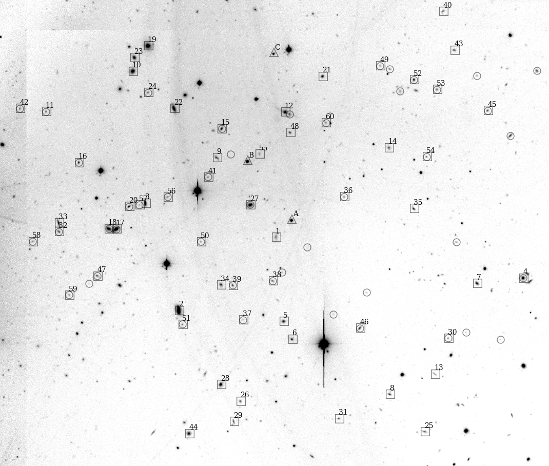
Figure 1: The CFHT imaging used to select galaxy candidates for the MOS observations. North is up and East is to the left. The field is around $10\times 8$ arcmin. Triangles show the QSOs, squares show galaxies with redshifts, and circles show objects targeted with the CFHT MOS. The numbers next to each square identify the galaxies in Table 2. Redshifts for objects with a square but no circle were provided to the authors by R. Weymann and M. Rauch. The proper CFHT baffles were absent during the imaging, causing the diffuse arcs of scattered light in the background.

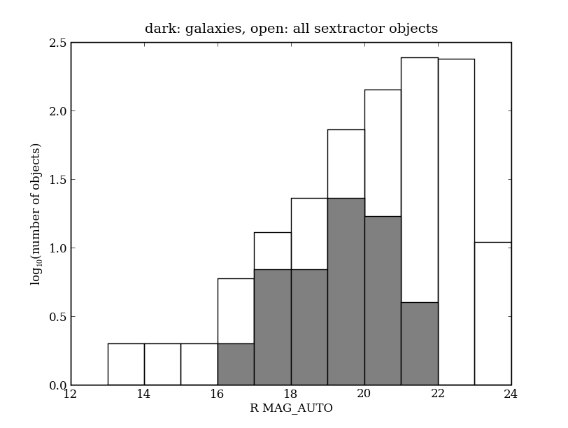
Figure 2: Number counts for the galaxies and SExtractor-selected objects. The grey histogram shows the number counts for galaxies with redshifts, the open histogram for all objects. The object catalogue list appears complete to R $=21.5$. The galaxy completeness drops significantly at R $>20.5$.

Figure 1 shows the imaging used to select galaxy candidates and the positions of galaxies with known redshifts. The proper CFHT baffles were absent during the imaging, causing the diffuse arcs of scattered light in the background. This scattered light makes it very difficult to assign a completeness limit to the imaging, as it affects some parts of the image more severely than others. SExtractor was used to create an object catalogue from the imaging. A histogram of number counts for SExtractor-identified objects roughly follows a power law up to magnitude of 21.5-22 before dropping. Thus we can say that the completeness drops significantly past R $=21.5$. The redshift sample completeness drops sharply past R $=20.5$ (see Figure 2). We note that the galaxy sample is not intended to be complete to a magnitude limit within some radius of the QSOs, and the distribution is roughly centred around LBQS 0107-025A, with very few redshifts north of LBQS 0107-0232.

The fraction of all possible galaxy candidates targeted for spectroscopy varied from $\sim 50\%$ for bright targets, to $<10\%$ for the faintest spectroscopic targets ($R\approx 21$).

2.2 QSOs and absorption line data

QSOs

This QSO triplet was discovered in the Large Bright Quasar Survey (Foltz et al., 1987). The positions and redshifts of LBQS 0107-025A (QSO A), LBQS 0107-025B (QSO B), LBQS 0107-0232 (QSO C) are given in Table 3. Their positions are also shown in Figure 1. The angular separations between the three QSOs are 1.29 arcmin (A–B), 1.92 arcmin (B–C) and 2.93 arcmin (A–C). One arcmin corresponds to a transverse separation of 190 kpc, 355 kpc and 455 kpc at redshifts of 0.2, 0.5 and 0.9 with our assumed cosmology.

The Ly$\alpha$ forest in each sightline of the two brighter QSOs, LBQS 0107-025A and LBQS 0107-025B, has been studied extensively (Dinshaw et al., 1995, 1997) using UV HST spectra. These analyses provided some of the first evidence for large scale ($\sim 400$ kpc) coherence in the Ly$\alpha$ forest. The analysis by Young et al. (2001) added HST spectra for the third nearby line of sight towards the QSO LBQS 0107-0232.

Absorption lines

Petry et al. (2006) used all the available UV HST Faint Object Spectrograph (FOS) and Goddard High Resolution Spectrograph (GHRS) spectra to create a catalogue of absorption lines seen in each QSO’s spectrum. LBQS 0107-0232 has observations from a single FOS wavelength setting covering the wavelength range 1572–2311 Å. LBQS 0107-025A and LBQS 0107-025B were both observed with three wavelength settings – one using GHRS (1212–1498 Å) and two using FOS (1572–2311 Å and 2222–3277 Å). The resolution of the FOS spectra is 1.39 Å and 1.97 Å (FWHM) for the lower and upper wavelength ranges. The GHRS spectra have a resolution of 0.8 Å. The final combined S/N per resolution element is $\sim 30$ for the FOS spectra and $\sim 8$ for the GHRS spectra. Table. 1 summarises the details of the UV QSO observations used in our analysis.

Petry et al. (2006) aimed to measure velocity coincidences between absorption across the three sightlines, and so they investigated and corrected several causes of velocity shifts between the different FOS spectra. We use their line wavelengths and fitted equivalent widths in our analysis. We verified that their line-detection algorithm was working correctly (and did not depend on, say, the method of combining the spectra or continuum fitting) by performing an independent combination of the archival FOS and GHRS spectra of the three QSOs, applying the wavelength shifts given by Petry et al. to each exposure. We confirmed that the lines they flagged as detections also appeared in our combined spectra.

The line positions and equivalent widths from Petry et al. (2006) along with our line identifications are listed in Tables 4 to 10. The equivalent widths and FWHM values in these tables are for the Gaussian line fitted to the feature. The detection significance is the equivalent width of a feature divided by the error in the equivalent width ($\sigma_{\rm det}$ – see Petry et al. for a more detailed description). We note that Petry et al. did not adjust the wavelength scales of the GHRS spectra.

Petry et al. did not search for metal lines inside the Ly$\alpha$ forest, other than rest wavelength galactic absorption. They also did not search for higher order Lyman series lines, rather showing that the number of lines in the Ly$\beta$ region was consistent with the expected $dN/dz$ for Ly$\alpha$ alone. Therefore, we made independent line identifications, guided by the Petry et al. and Dinshaw et al. (1997) line identifications. This was done by assuming every line blueward of the QSO Ly$\alpha$ emission was a Ly$\alpha$ transition, and searching for corresponding strong metal (C iv, Si iv, O vi, Si iii) and higher order H i Lyman series transitions within a narrow range around the expected redshift position. This process resulted in several new identifications compared to the Petry et al. line lists, generally higher-order Lyman series lines in the forest region. We also identified a number of strong low-ionisation metal lines associated with the Ly$\alpha$ line at $z=0.557$ towards QSO C. Although higher order Lyman transitions are not available for this system, it is likely a sub-DLA with $N_{\rm HI}$ $>10^{19}$ cm^-2. The associated strong Si ii, Si iii, Fe ii, C ii and O i lines suggest it may be similar to the super-solar sub-DLAs in Prochaska et al. (2006). These new identifications mean that several of the lines used in the analyses by Young et al. (2001) and Petry et al. (2006) were incorrectly assumed to be Ly$\alpha$. We discuss what implications this has for the Petry et al. (2006) results in Section 3. The line identifications are listed in Tables 4 to 10. In some cases absorption features appeared at the expected position of a metal line or higher order Lyman series line, but appeared to be blended with unrelated absorption. This is indicated in the tables by a ’?’ next to the line identification.

We checked the wavelength scales of the GHRS spectra by comparing the expected wavelengths of galactic lines (C ii 1334, Si ii 1260, Si iv 1393, O i 1302) and higher-order Lyman series lines with absorption appearing in the FOS spectra with the observed line positions.

For QSO B the Ly$\beta$, Ly$\gamma$, Ly-4 and Ly-5 transitions associated with the Lyman limit system at $z=0.3993$, and the galactic lines Si ii, O i, C ii and Si iv are seen in the GHRS spectra. We measure the difference between the expected position (corresponding to $z=0$ for galactic lines, and $z=0.3993$ for the Lyman series lines) and the observed central wavelength for a Gaussian profile fitted to each line. We then estimate a correction to the GHRS wavelength scale by taking the average of offsets for all these lines, excluding Si ii, Ly$\gamma$ and Si iv as they have either low S/N, poorly determined parameters, or are blended. We find a $-0.6$ Å offset from the expected line positions, thus we add 0.6 Å ($\sim 1$ resolution element) to the wavelengths given by Petry et al. We list our adjusted wavelengths for lines in the QSO B GHRS spectrum in Table 4.

For the QSO A GHRS spectrum the S/N is poorer and there are no clear, unblended higher order Lyman series lines that show Ly$\alpha$ in the FOS spectra. Lines near the positions of Galactic Si ii, O i, C ii and Si iv are present. However, Si ii is blended with unrelated absorption, and the remaining three lines do not give consistent shifts from the expected positions (O i: $-0.72$ Å, C ii: 0.0 Å and Si iv: $-0.18$ Å). As there is no clear offset, we decide not to apply a wavelength shift to the QSO A GHRS spectrum. Table 5 lists the (unshifted) wavelengths for lines in the QSO A GHRS spectrum. We note that a 0.5 Å shift corresponds to a velocity shift of $\sim 120$ km s^-1 at 1250 Å, thus even if some error in the GHRS wavelength scale remains, we are confident it is less than $\sim 200$ km s^-1.

The typical $1\sigma$ statistical error on the wavelength of an absorption line is  0.2 Å, corresponding to a velocity error of 30–50 km s^-1. Petry et al. estimate the FOS absolute wavelength calibration errors at $\sim 0.5$ pixels, or $\sim 32$ km s^-1. As we show above, any errors in the GHRS wavelength calibration are $<200$ km s^-1, and probably much lower than this. We expect the absorption line positions to have an error of $\sim 80$ km s^-1. This uncertainty is smaller than the typical galaxy redshift $1\sigma$ error of $\sim 180$ km s^-1.

To construct the sample of Ly$\alpha$ lines that we compare to galaxies, we select all lines that have been identified as Ly$\alpha$ and all unidentified lines. Finally, we remove any lines that are within 3500 km s^-1 of the QSO redshift. Lines close to the QSO emission redshift may be clustered around, ejected from, or ionised by radiation from the background QSO. Wild et al. (2008) measure an increase in CIV systems close to background QSOs due to both clustering and ejected aborbers. Based on their results, a 3500 km s^-1 cut should be ample to remove any clustered absorbers. It is also much larger than the scales on which we expect to see a significant reduction in the line density due to the proximity effect (e.g. Scott et al., 2002). Absorbers are known to have ejected velocities of more than 10000 km s^-1 in broad absorption lines quasars (e.g. Hamann, 1998). However, most ejected C iv absorbers have velocities $<3000$ km s^-1– Wild et al. find fewer than 40% of C iv systems at 3000 km s^-1 blueward of the QSO redshift are ejected. We believe 3500 km s^-1 is a reasonable compromise between excluding Ly$\alpha$ absorbers that arise in ejected systems without removing an excessive number of intervening IGM absorbers.

Our Ly$\alpha$ sample may not be the true Ly$\alpha$ sample for two reasons. Firstly, some unidentified lines may be due to transitions other than Ly$\alpha$. Secondly, some lines that have been identified with non-Ly$\alpha$ transitions may be blended with Ly$\alpha$ lines. In the first case our Ly$\alpha$ list may contain additional spurious Ly$\alpha$ absorbers, and in the second case we may have missed real Ly$\alpha$ absorbers. We believe the number of spurious Ly$\alpha$ lines is very low, given the low density of strong metal-bearing forest lines at these redshifts, and that we have searched thoroughly for galactic and extragalactic metal lines and higher-order Lyman lines in the forest. It is more likely that our list of Ly$\alpha$ lines is conservative due to the second case; we have missed some Ly$\alpha$ lines blended with other transitions. If we have missed lines, the correlation strengths we measure across sight-lines and with galaxies will be smaller than the true strengths. We may also underestimate the number of associated galaxy-absorber groups (see Section 4.4) over our redshift range due to missing some Ly$\alpha$ absorbers.

Optical spectra of QSOs A and B, taken with the Multiple Mirror Telescope Spectrograph, were presented in Dinshaw et al. (1997). These cover wavelengths from 3250–5650 Å at a resolution of 1 Å (FWHM) and a S/N of $\sim 10$, and they rule out any Mg ii absorption with rest equivalent width $>0.3$ Å from absorbers in the redshift range $0.34<z<1.02$.

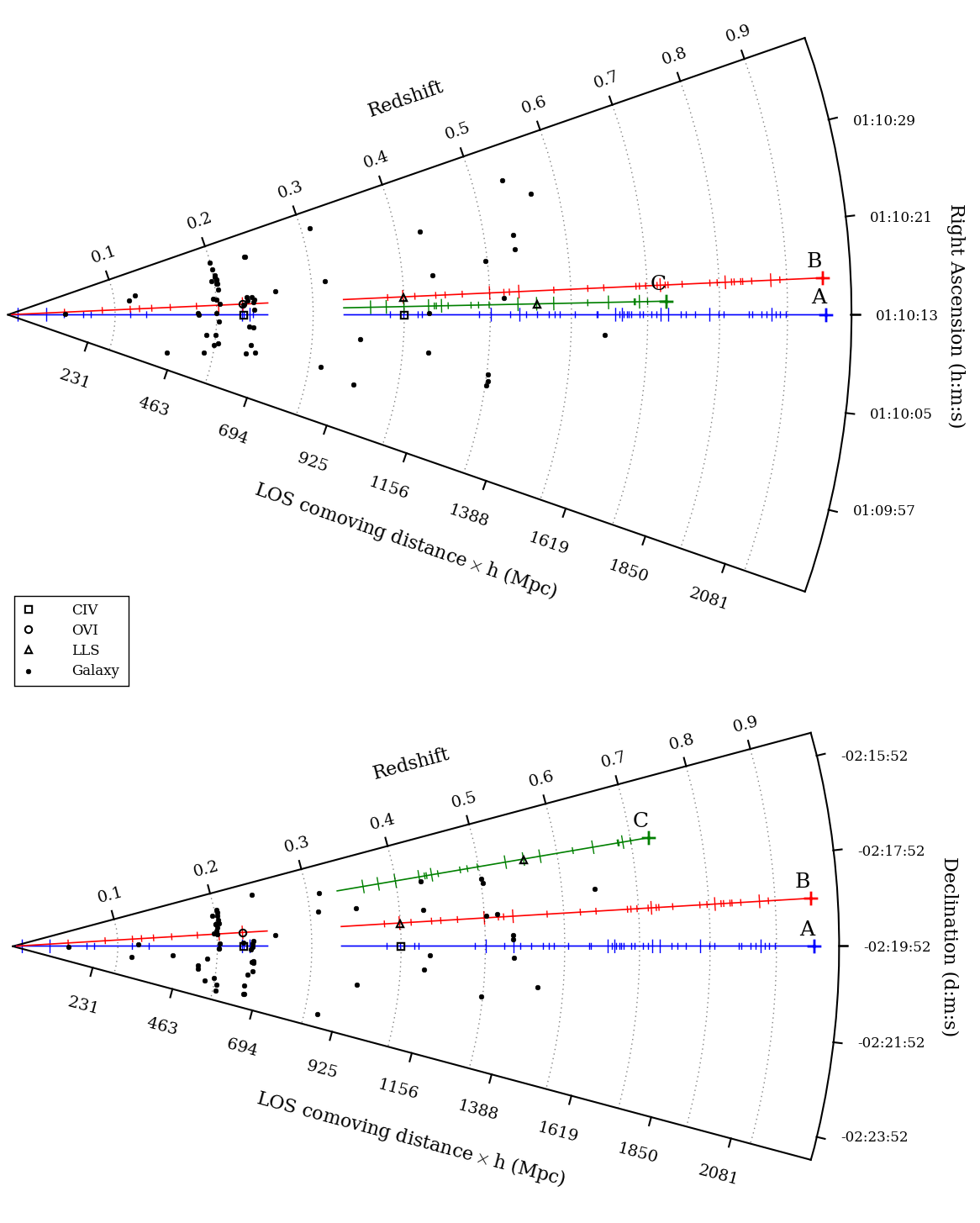
Figure 3: The distribution of galaxies and absorption lines in the Q0107 field. Angular separations have been exaggerated by 200 times to clearly separate the galaxy and absorber symbols. Galaxies are shown by black dots and the three QSOs are shown as plus signs. Absorbers along the QSO sightlines are shown by strokes perpendicular to the sightline: narrow strokes represent H i absorbers with rest EW $<1$ Å, wider strokes represent rest EW $\geq 1$ Å. The positions of O vi, C iv, the Lyman-limit system in sightline B and probable sub-DLA in sightline C are also shown (see the Figure legend).

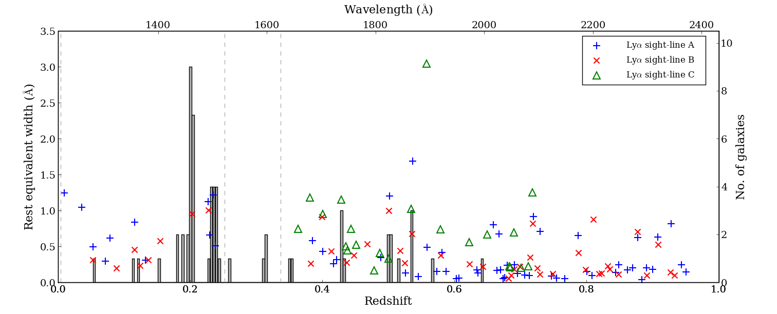
Figure 4: The redshift distribution of the galaxies and Ly$\alpha$ absorbers. The grey histogram shows our sample of galaxy redshifts. Plus signs, crosses and triangles show the Ly$\alpha$ absorber redshifts and their rest equivalent widths. The dashed lines show the cutoff wavelengths for the GHRS spectra and FOS spectra. QSO C was not observed with the GHRS, so there are no detected absorbers at redshifts $\lesssim 0.3$ in this sightline.

Wedge plots showing the Ly$\alpha$ lines a galaxy positions used in our analysis are shown in Figure 3, and Ly$\alpha$ rest equivalent widths, redshifts and the galaxy distribution are shown in Figure 4.

HST Observations
QSO Name Proposal Instrument Grating Exposure Wavelength S/N per Resolution Dispersion IDs Time (min) Range (Å) pixel FWHM (Å) (Å/pixel) Q0107$-$025A (A) 5172, 6260 GHRS G140L 549 1212–1498 5 0.8 0.143 5320, 6592 FOS G190H 448 1572–2311 28 1.39 0.36 6100 FOS G270H 146 2222–3277 22 1.97 0.51 Q0107$-$025B (B) 5172, 6260 GHRS G140L 337 1212–1498 7 0.8 0.143 5320 FOS G190H 108 1572–2311 13 1.39 0.36 6100 FOS G270H 107 2222–3277 34 1.97 0.51 Q0107$-$0232 (C) 6100, 6592 FOS G190H 548 1572–2311 16 1.39 0.36

Table 1: For the UV observations of each quasar we show the proposal ID numbers, the instruments and gratings used, the total exposure time, wavelengths covered, a representative S/N per pixel for a combined spectrum, and the resolution and dispersion. For more detailed information see Petry et al. (2006).

3 Re-analysis of H i Ly$\alpha$ coincidences across three sightlines

In this section we re-analyse absorber-absorber associations across the three sightlines using our new line identifications. We also describe a new way of classifying absorber coincidences across multiple QSO sightlines.

3.1 Re-analysis with new line identifications

Our identification of higher order Lyman series lines and metal lines in the forest of each QSO resulted in the identification of several lines assumed by Petry et al. (2006) to be Ly$\alpha$ that are in fact due to different transitions. Here we see what effect this has on their analysis, and discuss their method for selecting triple Ly$\alpha$ coincidences across the three sightlines.

Petry et al. (2006) identified absorber pairs and triplets across the three sightlines using nearest neighbour (NN) matching. When identifying absorber pairs, the NN match for a given absorber is the nearest absorber in velocity space in an adjacent sightline. Each absorber in a given sightline has two nearest neighbours; one for each remaining sightline. One might object to this matching method because it uses only the velocity separations, and not the angular separations when finding the nearest neighbour. Indeed, we could find the nearest absorber using the 3-d distance between each absorber pair instead of a velocity difference. For a flat universe, the 3-d distance can be found from the hypotenuese of the right angled triangle formed by the comoving separation in the redshift direction (assuming the velocity difference is due to some combination of the Hubble flow and peculiar motion) and the transverse separation between two absorbers. However, the transverse separations between the absorbers towards our QSOs (always $<0.5$ physical Mpc for our redshift range) are very small compared to the redshift separations (75 km s^-1 is $\sim 1$ Mpc at $z=0.15$, assuming pure Hubble flow). Therefore it is reasonable to use the velocity difference as a proxy for the 3-d separation. In addition, it is a simpler way of matching absorbers than finding the closest absorber in 3-d space, and has the advantage that it requires no assumptions about peculiar velocities.

Petry et al. also introduced a variant of nearest neighbour matching: symmetric matching. A symmetric Ly$\alpha$ pair is defined as a pair of absorbers that are nearest neighbours of each other. Unlike NN matches, where a single absorber can be a member of many NN pairs, a given absorber can be a member of only one symmetric pair. They use symmetric matching to identify absorber triplets in a way that makes no assumptions about the velocity offset between the members of a triple. A symmetric triplet is defined as a group of three absorbers, one in each sightline, that are all NN of each other. They detect 12 such triplets, and find that this number is significant at the $>99.99$% confidence level compared to random Monte Carlo absorber simulations.

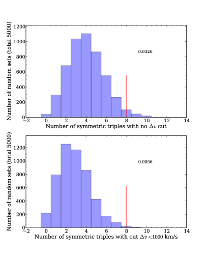
Figure 5: Top: The number of symmetric triples across the three sightlines for a thousand sets of random absorbers and the real absorbers with our new line identifications (vertical line). This figure is directly comparable to Petry et al.’s Figure 11. The probability of matching or exceeding the number of triples in the real absorbers by chance is shown in the top right-hand corner; 3.3%. Bottom: Similar to the top panel, but showing only symmetric triples containing pairs with velocity separations less than 1000 km/s. The significance has increased compared to the top panel.

Using our new identifications we find three of these 12 symmetric triplets contain lines that are not due to H i Ly$\alpha$. We note that two of these three have large velocity separations between the absorbers that make up the triples – 1062 km s^-1 and 814 km s^-1 – consistent with them containing a spurious line. A fourth triplet is removed as it contains a line with detection significance of 2.16$\sigma$, less than our cutoff detection significance of 3$\sigma$. We are left with eight triplets, shown in Table 11. Using our own Monte-Carlo simulations (see Appendix A) we find at least this number of symmetric triplets in 163 out of 5000 random sets, giving a significance level of 96.7%, somewhat lower than the significance reported by Petry et al. (see the top panel of Figure 5). Note that even though four of the triplets have been removed, the significance level remains at the 97% level as there are fewer Ly$\alpha$ lines in total, increasing the significance of any matches. Thus the significance of the Petry et al result is reduced, but not entirely removed by the new line identifications.

Advantages and disadvantages of symmetric triple matching

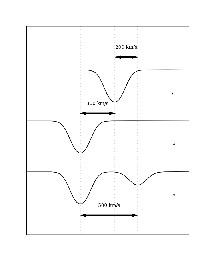
Figure 6: An example of a physically plausible group of absorbers spanning three sightlines that is not selected using the symmetric triple matching algorithm from Petry et al. (2006), as there is no combination of three lines that are all nearest neighbours of each other. This system is selected by our group selection algorithm. (Note that lines with $\approx 500$ km s^-1 separations are clearly separated in a single sightline, even in the moderate resolution FOS spectra).

While following the Petry et al symmetric matching procedure, we discovered two potential problems with this matching algorithm. Firstly, a small but significant proportion of the symmetric triplets we find in the random absorber sets have unphysically large velocity separations (larger than 4000 kms, or $\gtrsim 50$ Mpc assuming no peculiar velocity contribution). Secondly, there are configurations of absorber groups that span the three sightlines and have plausibly small velocity separations, but will not be detected by the symmetric matching method. An example of such a configuration is shown in Figure 6. Finally we found that if there are large gaps in the spectral coverage, the symmetric matching method will identify many spurious triplets that are comprised of absorbers matched across the gaps. We can minimise the number of such spurious triplets by restricting our analysis to ranges where we have complete wavelength coverage across the three sightlines. However, it is worth noting that this matching method is best suited to spectra with a similar, continuous wavelength coverage across each sightline, with slowly-varying detection limits.

To address the problem of triplets with spuriously large velocity separations we can add a velocity cut criterion to the symmetric matching algorithm, and only accept triplets with a maximum velocity difference between any two triplet members below some cutoff value. Petry et al. applied a 400 km s^-1 velocity cutoff when comparing equivalent widths of members of symmetric triplets in the real absorbers to those in the random sets. The bottom panel of Figure 5 shows the result of applying a cut of $\Delta v<1000$ km s^-1. No symmetric triples in the real absorbers are removed with this cut but many random symmetric triples are removed, so the significance level increases to $>99$%. We could vary the cutoff velocity difference to maximise the significance level of the observed triplets, but this a posteriori choice of a velocity cut is unsatisfying. In addition, applying a velocity cut undermines one of the appealing characteristics of the symmetric matching method: that it makes no assumption about the velocity difference between triplet members.

Thus we conclude that using the symmetric matching method there is still very strong evidence ($>99$% confidence) for absorbing structures across the three sightlines with typical velocity separations smaller than $1000$ km s^-1. However, the problems with the symmetric matching described above led us to explore a different method of identifying absorber triplets, which we describe below.

3.2 A new method for identifying absorber coincidences in multiple sightlines

In this section we explore a different algorithm for detecting triple line coincidences. It uses only a velocity cut to identify groups of absorbers, without any nearest-neighbour matching.

The algorithm consists of the following steps: first a maximum velocity separation, $\Delta v_{\rm max}$, is specified. Next we step through each Ly$\alpha$ absorber redshift in each sightline, and search for absorbers in all three sightlines that have an absolute velocity separation less than $\Delta v_{\rm max}$ from this redshift. All absorbers that satisfy this condition are placed into a provisional absorber ‘group’. This process creates one ‘group’ for each absorber that contains one or more absorbers across one, two or three sightlines, all with velocity separations less than twice $\Delta v_{\rm max}$. Finally, to avoid counting the same structure multiple times, we remove any group whose members are all members of another single group (however, it is still possible for a single absorber to be the member of more than one group).

This process locates triples classified using symmetric matching that have a maximum velocity separation between their members that is less than $\Delta v_{\rm max}$. It also finds configurations that symmetric matching will miss (such as the example in Figure 6), and naturally selects pairs of absorbers across each set of two sightlines.

We measure the number of absorber groups containing at least one absorber in each sightline for both the real and random absorbers for three different $\Delta v_{\rm max}$ values: 200, 500 and 1000 km s^-1. Table 11 shows all the lines that are members of triple groups founds with $\Delta v_{\rm max}=200$ km s^-1 and $\Delta v_{\rm max}=500$ km s^-1. The velocity cut method finds all but one of the triples found using the symmetric matching method for $\Delta v_{\rm max}=500$ km s^-1. Although it is possible for multiple absorbers in a single sightline to be part of a single triple (this was a motivation for using the new algorithm), all of the triples found below a $\Delta v_{\rm max}$ of 500 km s^-1 have only a single absorber in each sightline.

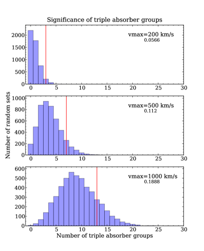
Figure 7: The number of triple absorber groups in the real absorbers compared to the number found in random absorber sets for three maximum velocity differences between the absorber group members. The histograms show triple groups in the random sets, and the vertical line shows the triple groups in the real absorbers. The probability of matching or exceeding the number of triples in the real absorbers based on the distribution of the random absorbers is shown on each panel. There is marginal evidence for an excess of triple absorber groups identified using vmax $=200$ km s^-1 (significance of 94.7%).

The number of groups found across all three sightlines in the real absorbers compared to the number found in random absorber sets are shown in Figure 7. There is a marginally significant (94.3%) excess of real absorber triples compared to the random sets for $\Delta v_{\rm max}=200$ km s^-1, with the significance decreasing for $\Delta v_{\rm max}=500$ km s^-1 (89%) and $\Delta v_{\rm max}=1000$ km s^-1 (81%). This is a less significant result than that for triplets identified with symmetric matching. If real physical structures create configurations such as in Figure 6, then symmetric matching will miss these structures, and this lower significance level is a more accurate estimate of the probability that there are physical structures spanning the three sightlines.

It is also possible that the configurations missed using symmetric triple matching are not found in real observations – perhaps there are instrumental or physical reasons why the pairs of absorbers comprising triple coincidences are unlikely to be found with small separations, making configurations such as that shown in Figure 6 unlikely. One possibility is that compared to the random absorbers, real absorbers are less likely to be found with small separations in the same sightline due to line blending – for example, two lines might be fitted as a single broad line if their separation is smaller than the FWHM resolution of the FOS spectra (1.29 Å, or $\sim 230$ km s^-1 at 1700 Å for the G230M grating). To check the minimum wavelength difference at which lines can be separated within a single sightline, we measured the wavelength difference between adjacent lines within each sightline over the G230M wavelength range. The minimum separation between any two adjacent lines (not only Ly$\alpha$ transitions) is 1.8 Å, or 320 km s^-1 at 1700 Å. The minimum separation we allow between lines in the same sightline in our random absorber catalogues is 2.0 Å (see Appendix A), thus we do not expect real absorbers to have fewer closely separated lines within a given sightline than the random absorbers due to this effect. Another possibility is that absorption lines caused by structures spanning the three sightlines are ‘isolated’, and less likely to show multiple absorption components over such small velocity ranges within each sightline. However, there is no evidence in the literature for reduced power in the Ly$\alpha$ auto-correlation function on these scales.

In summary, our new method for selecting coincident absorption across the three sightlines finds evidence at the $94$% confidence level for absorbing structures that span the three sightlines. This is a lower significance than the symmetric triple matching method ($97-99$%).

3.3 The rest equivalent width of symmetric triplet members

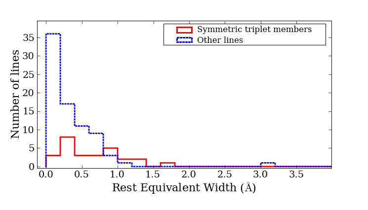
Figure 8: The distribution of rest equivalent widths for members of symmetric absorber triplets (solid histogram) and lines not in triplets (dotted histogram). There is a visual impression that absorbers in symmetric triples have a higher equivalent width than the absorbers, but the number of lines is small, and a K-S test does not suggest the distributions are significantly different.

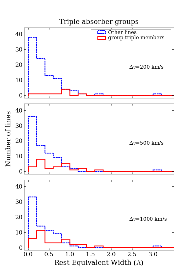
Figure 9: The distribution of rest equivalent widths for members of absorber group triples (solid histogram) and lines not inside group triples (dotted histogram) for three velocity cutoffs. Again there is a visual impression that triple group members are more likely to have higher rest EWs, particularly for the $\delta v=200$ km s^-1, but a K-S test does not suggest the distributions differ significantly.

The methods used above to identify absorber coincidences do not take into account the equivalent width of lines comprising triple absorber coincidences. Petry et al. (2006) find that members of symmetric triplets in the real absorbers have larger equivalent widths (averaged over members of each triplet) compared to triplets found in the random absorber sets. We find that this relationship still holds with our new group identifications. We also measure the rest equivalent width of lines that are members of symmetric triplets and compare this to the rest EW of lines that are not members. Figure 8 shows the results: the number of lines are small, and a Kolmogorov-Smirnov (KS) test gives a $68$% probability that both data sets are drawn from the same distribution, thus there is no evidence that members of triplets have a significantly different rest EW to non-members. We repeat the same test using lines inside and outside the triple groups identified using our matching method. Figure 9 shows the result. Again the number of lines is very small, and a KS-test cannot rule out the two data sets coming from a single distribution.

4 Galaxy-absorber associations

We have seen that identifying structures that span the three QSO sightlines using H i absorption alone is difficult due to the small numbers of absorber coincidences and the relatively weak correlation of Ly$\alpha$ absorbers. This is a further motivation for adding the galaxy positions to our analysis – adding more statistical power to search for large scale structures. In the following sections we give a qualitative description of the observed groups of galaxies and absorbers, look at the associations between metal line systems and galaxies, describe the statistical tests we use to measure the extent of any absorber-galaxy association, and present the results of these tests.

4.1 Initial impressions

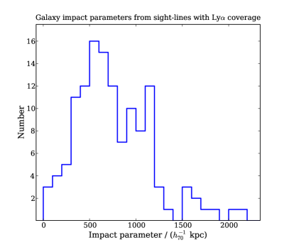
Figure 10: The distribution of impact parameters of galaxies from all three sightlines where there is coverage of the Ly$\alpha$ line corresponding to the galaxy redshift.

Of our 60 galaxies with redshifts, 56 are at redshifts with overlapping Ly$\alpha$ coverage in at least two QSO sightlines. Of these 56, 22 have impact parameters $\rho<500$ kpc from their nearest sightline, and 5 have $\rho<200$ kpc. The distribution of galaxy $\rho$ from all of the three sightlines where there is Ly$\alpha$ coverage is shown in Figure 10.

Before we describe our statistical tests for galaxy-absorber associations, we look more closely at the wavelengths corresponding to Ly$\alpha$ absorption in the QSO spectra close to galaxy redshifts. The series of plots in Figure 11 shows $\sim 6000$ km s^-1 spectral regions around one or more galaxies that overlap with spectra in two or more sightlines. In general, all the galaxies shown in a single plot are within a 1000 km s^-1 velocity range, with the exception of the $z=0.19$ group, which consists of three pairs of galaxies that are spread across 4000 km s^-1. The left panels show the galaxy distribution relative to the QSO sightlines in right ascension and declination. The transverse distances given are physical distances relative to the B sightline at the redshift of each galaxy. The size of the galaxy symbols are proportional to the galaxy luminosity (though note the uncertainties in the absolute B magnitudes in Table 2), and colour shows the relative velocity offset. The velocity zero point is at the mean redshift of Ly$\alpha$ lines overlapping with the galaxies, or the mean redshift of the galaxies if no line overlaps. The open circle in the top left corner shows the size of an L* galaxy for comparison. We found the Schechter function parameter M*$(z)$ in the $b$ band by interpolating in redshift across the DEEP2 values given in Table 4 of Faber et al. (2007) and assuming M*$=-20$ at $z=0$. Galaxies are marked by their numbers from Table 2. If there is any H i Ly$\alpha$ absorption along a sightline within 1000 km s^-1 of the zero velocity position it is shown by an inverted triangle. The area of the triangle is proportional to the summed Ly$\alpha$ rest equivalent width. If no Ly$\alpha$ absorption is detected within this range, the position of the sightline is shown by a plus sign.

The right panels show portions of spectra corresponding to H i Ly$\alpha$ overlapping in velocity space with the galaxies in the left panel. Our combined spectra and fitted continua are shown, with the lines identified by Petry et al. shown as vertical tick marks. Solid tick marks are lines in our Ly$\alpha$ list and dotted tick marks are lines that have been attributed to a transition other than Ly$\alpha$. Lines are marked by their numbers from Tables 4 – 8. Petry et al. used a slightly different method to combine the spectra and fit the continuum, thus there may be small differences in the apparent significance of lines in these plots compared to Tables 4 – 8. The nearby galaxy positions are shown as small triangles at zero flux in each spectrum. Filled triangles are galaxies that are also shown in the corresponding left panel. In Appendix B we comment on each of the Figure 11 plots individually.

There are several candidates for physical associations between absorbers and nearby galaxies. There are two large groups of galaxies, one at $\langle z\rangle=0.202$ and another over the range $z=0.233-0.238$. Both of these groups are near sightlines A and B, where the GHRS spectra cover the expected Ly$\alpha$ positions. Both groups show strong (rest EW $>0.3$Å) Ly$\alpha$ absorption in one sightline, but no strong absorption in the neighbouring sightline.

One faint ($\sim 0.03$ L*) galaxy at $z=0.053$ is within 30 kpc of sightline A and 100 kpc of sightline B. Ly$\alpha$ absorption is seen in both sight lines at the galaxy’s redshift. Unfortunately we do not have access to a spectrum of this galaxy, and so cannot examine its properties in detail. Another brighter galaxy ($\sim 1.2$ L*) at $z=0.227$ is $170$ kpc from sightlines A and B. Very strong Ly$\alpha$ absorption (rest EW $>1$ Å) is seen in both sightlines within 200 km s^-1 of the galaxy redshift. We do have a spectrum of this galaxy and we use it to constrain the galaxy’s star formation history in Section 4.2.

There is also an example of a galaxy close to a sightline that does not show associated strong Ly$\alpha$ absorption: the galaxy at $z=0.197$ is only 110 kpc away from sightline B, but there is no Ly$\alpha$ absorption with rest EW $>0.2$Å within 400 km s^-1 of the galaxy redshift. We note that there is absorption about 600 km s^-1 from the galaxy redshift that has been identified as Ly$\gamma$ from a higher-redshift absorber that may be masking Ly$\alpha$ absorption. If there is no Ly$\alpha$ absorber associated with this galaxy, this means that a simple model of each galaxy surrounded by a spherical halo of HI gas that always gives rise to absorption in a nearby sightline cannot explain the data without some modification (such as a variable covering factor).

4.2 Galaxies and metal line systems

There are six QSO absorption systems that show associated metal lines. Five of these were identified in Petry et al.; the sixth is the new sub-DLA we have identified towards QSO C. The lines comprising each system are listed in Table 12. One of the systems is a previously known ‘grey’ Lyman limit system, the other is the new sub-DLA system we discovered. At the moderate FOS and GHRS resolutions, column densities and velocity widths of lines cannot be easily measured, so we have no detailed information about the ionisation state or metallicity of the systems. However, we can look at their distribution relative to the galaxies and across sightlines.

It is interesting that every metal-line system in sightlines A and B has a H i Ly$\alpha$ line within $300$ km s^-1 in the nearby B or A sightline. Given the minimum rest equivalent width of an absorber containing a metal line ($\sim 0.45$ Å) and the number of absorbers above this rest EW in each sightline that have Ly$\alpha$ with 300 km s^-1 in the nearby sightline, we calculate the probability of this occurring by chance is less than $3.5$%. This is consistent with these metal line systems being associated with H i gas structures spanning the size of the sightline separations ($300-400$ kpc). However, absorbers with strong metal systems are not expected to be part of a single coherent structure so large – indeed, sub-DLAs are thought to be much smaller structures with typical sizes of a few tens of kpc. An alternate explanation is that such absorbers trace the halos of galaxies that are themselves embedded in a $\sim 0.5$ Mpc structure.

No galaxies are seen close to the LLS in sightline B or the sub-DLA in sightline C. High $N_{\rm HI}$ absorbers are sometimes found close to faint dwarfs (Rao et al., 2003; Stocke et al., 2004). However, such galaxies are too faint to have been targeted in the available spectroscopy samples. There are several faint galaxy candidates in the imaging shown in Figure 1 close to both sight lines. Typical impact parameters of galaxies that have been found close to LLS and DLAs range from $<10$ kpc (Gharanfoli et al., 2007) to 90 kpc (Jenkins et al., 2005). This corresponds to a separation from the QSO sightline of $~{}1-10$ arcsec. It is also possible that an associated galaxy might be blended with the QSO in our ground-based imaging.

A bright galaxy with nearby metal absorption at $z=0.227$

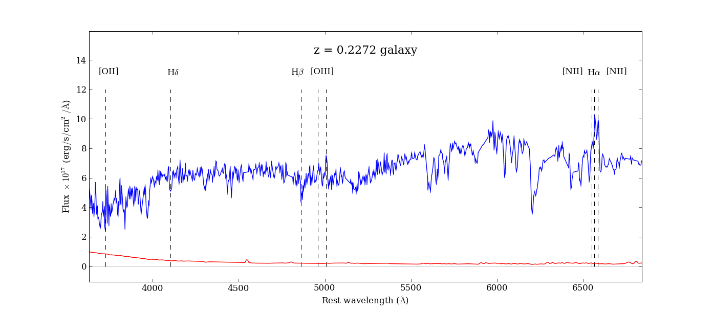
Figure 12: CFHT MOS spectrum of the $z=0.2272$ galaxy that has nearby metal absorption in QSO sightlines A and B. The flux is plotted as a function of rest wavelength, and the $1\sigma$ errors are shown. Features used in our analysis are labelled.

This a single bright ($1.2$ L*) galaxy at $z=0.2272$, 200 kpc from sightlines A and B. There are two strong (rest EW $\sim 1$ Å), broad Ly$\alpha$ absorbers (FWHM $2.26\pm 0.86$ and $3.44\pm 1.60$ Å, or $\sim 450$ and $\sim 690$ km s^-1) in each sight line within 200 km s^-1 of the galaxy position. The large rest EW and velocity width suggest the H i absorption is made up of several velocity components. Both the absorbers in sightlines A and B show associated metal absorption: O vi and C ii is seen in sightline B (though the S/N is low at the wavelengths of these lines and O vi appears blended with unrelated Ly$\alpha$); C iv and possibly C ii is seen in sightline A. H$\alpha$ and [O iii] emission in the galaxy’s spectrum (Figure 12) show it is undergoing some star-formation, and H$\beta$ absorption shows there is a population of young and intermediate age stars.

We quantify the star-formation history of the galaxy by measuring the H$\alpha$, [N ii], [O iii] and [O ii] emission line intensities, the continuum drop over the 4000 Å break quantified by the D(4000) parameter, and the H$\delta$ absorption line rest equivalent width (H$\delta$_A index).

Kauffmann et al. (2003) show that D(4000) and H$\delta$_A can be used to discriminate between two galaxy star formation scenarios. The first scenario models the star formation rate (SFR) in a galaxy as decreasing exponentially from some initial formation time. The second has the same decreasing SFR along with randomly-occurring bursts of star formation.

The H$\delta$_A index (as used by Kauffmann et al.) is defined in Worthey & Ottaviani (1997) as the rest equivalent width of the H$\delta$ line from $4083.50-4122.25$Å. The continuum over the line is defined using the adjacent regions $4041.60-4079.75$ Å and $4128.50-4161.00$ Å. Two continuum reference points are calculated using the mean flux and mean wavelength in each of these regions. The continuum over the H$\delta$ line is then given by a straight line joining these two reference points.

D(4000) was first described in Bruzual A. (1983). It is the ratio of average flux densities $F_{\nu}$ above and below the 4000 Å break. We measure average flux densities using rest-frame wavelength ranges $3850-3950$ Å and $4000-4100$ Å (Balogh et al., 1999).

We find the $z=0.2272$ galaxy has H$\delta$${}_{A}=2.0\pm 0.5$ Å, and D(4000)$=1.28\pm 0.03$. These are formal errors from the $1\sigma$ flux errors, and the true errors are likely to be somewhat larger due to emission or absorption in the continuum regions. Figure 13 shows the values for this galaxy overlayed on a reproduction of Kauffmann et al.’s Figure 6, we find that this galaxy falls near a region where 95% of the model galaxies have not experienced bursts of star formation in the last 2 Gyr.

The H$\alpha$ emission line allows us to make a rough estimate of the star formation rate. Nebular lines originate in gas surrounding recently-formed stars, and thus their intensity gives a direct measure of the star-formation rate of the galaxy (subject to many potential pitfalls outlined in e.g. Kewley et al. 2002). We do not correct for absorption from dust. There is no measureable H$\beta$ emission, and thus we cannot use the difference between the expected and observed ratio of H$\alpha$ to H$\beta$ intensities to correct for any dust reddenning. Since there is Balmer absorption visible at H$\beta$ and H$\gamma$ it will also be present at H$\alpha$, and so our line intensity measurements will be smaller than the true intensity.

Mindful of these limitations, we used H$\alpha$ line flux to measure a star formation rate. We modelled the blended H$\alpha$ and nearby [N ii] lines with Gaussians, and use the deblended Gaussian to measure the H$\alpha$ line intensity. We fitted the continuum level around the emission lines using a median filter, measured the summed flux over the H$\alpha$ line, and then converted to a luminosity using the relations given in Section 1. Using the conversion relation from Kennicutt (1998), SFR (M_☉ yr^-1)$=7.9\times 10^{42}L(\hbox{{\rm H}$\alpha$})$ (erg s^-1), we found a star formation rate of 0.45 solar masses per year. This is relatively small for a late-type galaxy, but normal for an early-type.

Using the relations in Kewley & Dopita (2002) (their Figures 7 and 8) we can estimate the oxygen abundance, (O/H), in the galaxy’s nebular regions using ratios of the line intensities of [O iii], [N ii] and H$\alpha$. Keeping in mind that we have not corrected for reddening or Balmer absorption, we measure the ratios [N ii] $\lambda 6583$ / H$\alpha$ $=0.9$ and [N ii] $\lambda 6583$ / [O iii] $\lambda 5007$ $=2.4$. The [N ii]/H$\alpha$ is surprisingly large, which is indirect evidence that there is significant Balmer absorption at H$\alpha$, and that the star formation rate is higher than 0.45 M_☉ yr^-1. If we assume that the true H$\alpha$ intensity is five times larger than the measured intensity we find a range $8.5<$ log(O/H)$+12<9.4$. For [N ii]/[O iii] we find a range $8.2<$ log(O/H)$+12<9.2$. Thus it is likely that the galaxy’s (O/H) is larger than half solar, taking the solar oxygen abundance log(O/H)$+12=8.66$ from Asplund et al. (2004). These values are also consistent with the galaxy having undergone the bulk of its star formation more than $1-2$ Gyr ago.

The imaging is too poor quality to differentiate whether the galaxy is an elliptical or spiral based on its surface brightness profile. A fainter, stellar object is also seen very close to the galaxy, and this object fell inside the slit targeting the galaxy. We are unsure of its redshift, but the R band imaging suggests it does not contribute a significant amount of flux to the galaxy spectrum.

We could imagine the following scenario for this galaxy, consistent with the derived values above: a significant burst of star formation occurred more than 2 Gyr ago, producing metal-enriched gas that was ejected by winds. It is possible that the metals observed in the two nearby sightlines were created by these winds: an average wind speed of 100 km s^-1, typical of superwinds that can be associated with strong bursts of star formation, is equivalent to 100 kpc per Gyr. This is only one scenario; an equally plausible explanation for the enriched gas would be that it is more closely associated with galaxies our survey has missed. Interestingly both absorbers show absorption by high and low ionisation species metals, suggesting a multiphase environment.

4.3 Statistical tests for absorber-galaxy associations

There are two ways to approach a joint analysis of the galaxies and absorbers. The first asks the question: given the galaxy distribution, how likely are we to see the observed distribution of absorbers? The second asks: given the absorber distribution, how likely are we to see the observed galaxy distribution? We are currently obtaining a deeper sample of galaxy redshifts over a larger area in this field using the VIMOS and DEIMOS spectrographs, which will allow us to better address the second question in a future paper. However, since our knowledge of the selection function for our absorption lines is much better than that of our current galaxy sample, in this paper we focus on the first question.

We use two statistical matching methods to identify associations between galaxies and absorbers. The first uses a nearest-neighbour matching algorithm to link galaxies and absorbers, the second uses a velocity cut and identifies absorbers across all three sightlines that are associated with a galaxy. Both tests compare the number of galaxies with nearby absorbers using the real absorber distribution, and an ensemble of 5000 random absorber distributions. The method we use to generate random absorbers is described in Appendix A.

For the first matching method we identify the nearest Ly$\alpha$ absorber in each sightline to each galaxy in velocity space. We refer to this as a nearest neighbour absorber (NNA). We do this both for the galaxies and real absorbers, and the galaxies with each set of random absorbers. We compare the distributions of velocity differences between galaxies and their NNAs in the real and random absorbers.

The second matching method identifies galaxy-absorber ‘groups’ in a way similar to that we used to identify absorber groups in Section 3. We step through each galaxy redshift and assign every Ly$\alpha$ line in any sightline that is within some velocity range, $\Delta v$, of that galaxy as an absorber associated with that galaxy. Thus we have one ‘group’ for each galaxy, consisting of the galaxy and zero or more absorbers in zero to three sightlines with which it is associated. Note that absorbers can be ‘associated’ with more than one galaxy. We do this for both the real absorbers and random absorbers and compare the group properties between them.

We attempted to use nearest-neighbour matching methods to link a galaxy with absorbers in more than one sightline, but found that the above ‘group’ finding method was simpler to explain and implement, and should be more clearly linked to physical structures.

4.4 Results

Using the statistical tests described above, we compare the associations between galaxies and absorbers for the real absorbers and random absorber sets.

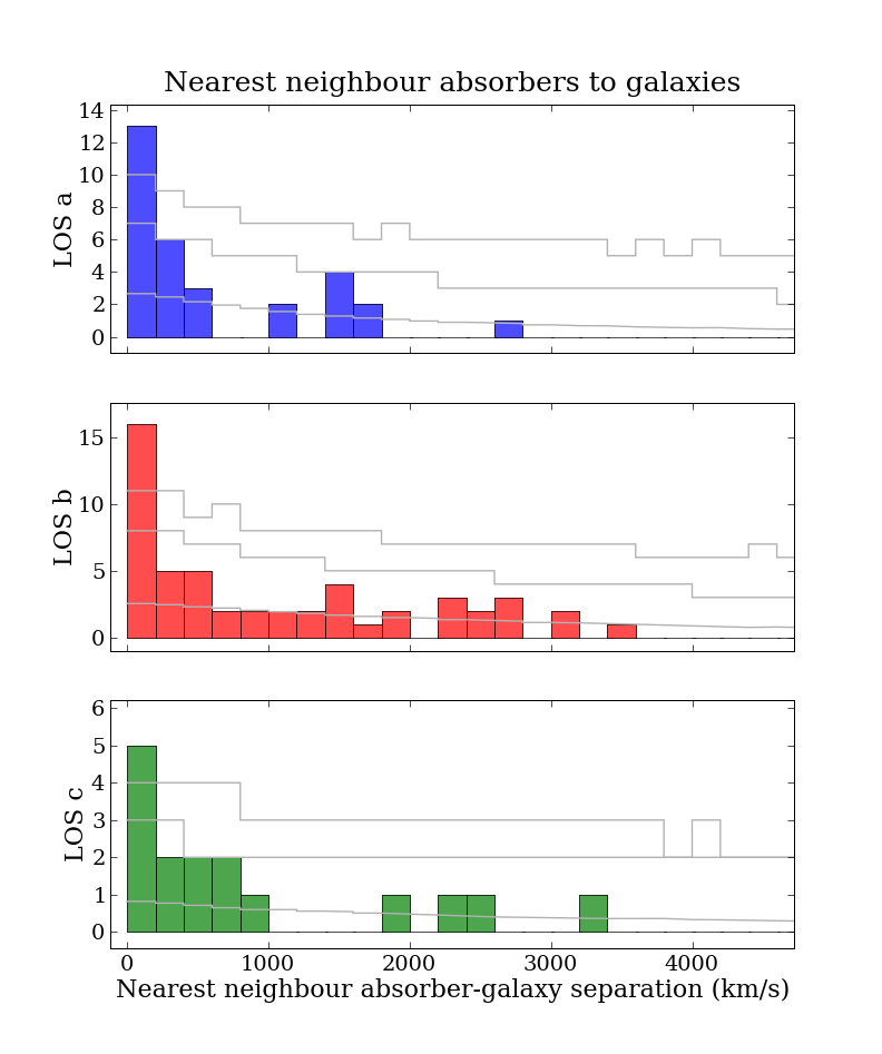
Figure 14: The number of galaxy-absorber nearest neighbour pairs (one for each galaxy) as a function of pair velocity separation for each sightline. The velocity bins are 200 km s^-1 wide. In each panel the thin grey lines show the mean number of pairs constructed using the same galaxy sample with 5000 random sets of absorbers (bottom line), the 95% confidence level from the random pairs (middle), and the 99% confidence level (top). There is a significant ($>99$%) excess of pairs compared to the random pairs at velocity separations $<200$ km s^-1 in all three sightlines.

First we use nearest-neighbour matching, looking at the smallest distance of a galaxy from an absorber in velocity space in each sight line. Figure 14 shows the results – there is a clear excess ($>99$% significance) of pairs at galaxy-absorber velocity separations $<200$ km s^-1 compared to the random absorbers in all three sight lines. The signal is slightly weaker for sightline C, likely due to the smaller wavelength overlap of the C spectrum with the galaxy distribution. The excess at $\Delta v<200$ km s^-1 is consistent with the excess of galaxy-absorber pairs in the larger sample of (single) QSO sightlines and galaxies in Morris & Jannuzi (2006, see their Figure 25). This is expected, as a large fraction of the data used in this paper is included in their analysis.

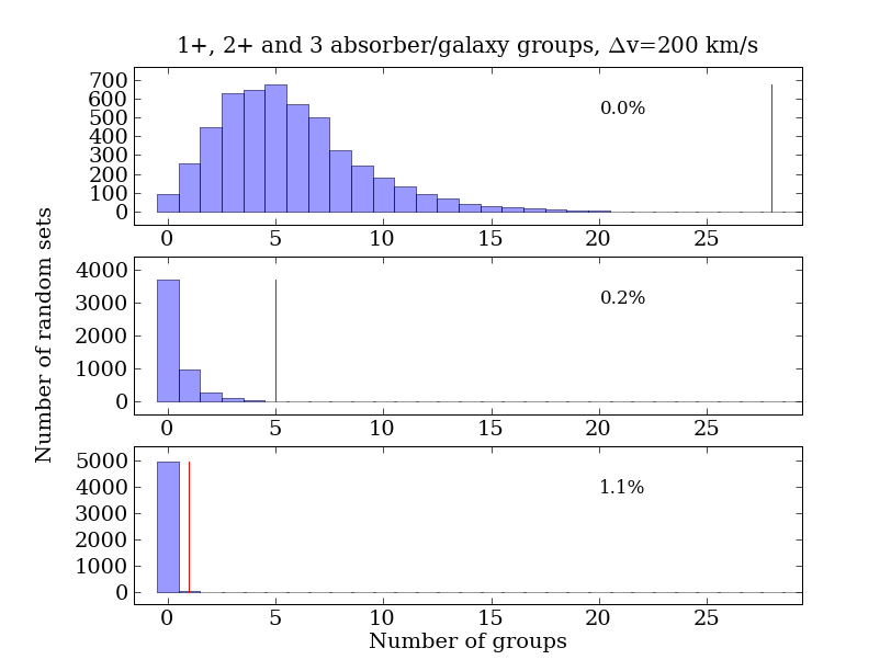
Figure 15: The number of galaxy-absorber ‘groups’ (defined in Section 4.3) using the real galaxies and real absorbers and maximum velocity difference of 200 km s^-1, compared to the number measured using the real galaxies and 5000 sets of random absorbers. The histogram shows the number of galaxies with associated absorbers in at least one (top), two (middle) and three (bottom) sightlines for random absorbers. The vertical line shows the number of groups using real absorbers. The probability of the real number arising by chance is shown in each panel (0.0% means none of the 5000 galaxy-random absorber sets had that many groups, i.e. $<0.02$%). There is a clear excess of galaxies associated with absorbers across one and two sightlines compared to random absorbers.

Next we look at the statistics of galaxy-absorber groups for a variety of velocity cutoffs. We make comparisons of three quantities between the observed and random sets: the number of galaxies with at least one associated absorber (in any sightline), the number of galaxies with associated absorbers in at least two sightlines, and the number of galaxies with associated absorbers in all three sightlines. We refer to these three types of groups as single-LOS galaxy groups (here LOS is an abbreviation for line-of-sight), double-LOS galaxy groups and triple-LOS galaxy groups respectively. We measure the number of such groups using velocity cutoffs for absorber-galaxy associations (as described in the previous section) of 200, 500, 750 and 1000 km s^-1. The results are shown in Figures 15 to 18. There is a significant (generally $>99\%$) excess of galaxies with associated absorbers in one, two and three sightlines compared to the random galaxy-absorber groups. Note that while 56 galaxies have overlapping spectra covering H i Ly$\alpha$ in two sightlines, only 16 galaxies have three sightlines overlapping in Ly$\alpha$. Thus statistics are poorer for the triple LOS-galaxy groups.

5 Comparison with simulations

In this section we compare the observations with the distribution of gas and galaxies within cosmological hydrodynamic simulations; for this task we use the Galaxies-Intergalactic Medium Interaction Calculation (Gimic; Crain et al. 2009). Gimic is designed to circumvent the large computational expense of simulating large cosmological volumes ($L\gtrsim 100$ $h^{-1}$ Mpc) at high resolution ($m_{\rm gas}\lesssim 10^{7}$ $h^{-1}$ M_⊙) to $z=0$.

Using ‘zoomed’ initial conditions (Frenk et al., 1996; Power et al., 2003; Navarro et al., 2004), Gimic traces with full gas dynamics the evolution of five roughly spherical regions drawn from the Millennium simulation (Springel et al., 2005). In order to trace a wide range of large-scale environments, the regions were chosen such that their overdensities deviate by (-2, -1, 0, +1, +2)$\sigma$ from the cosmic mean, where $\sigma$ is the rms mass fluctuation, on a scale of $18$$h^{-1}$ Mpc, at $z=1.5$. The $+2\sigma$ region was additionally constrained by the requirement to be centred on a rich galaxy cluster halo. In practice this ensures that the simulations include rare cosmological features, since the $-2\sigma$ region is also approximately centred on a sparse void.

Each region has an approximate comoving radius of $18$ $h^{-1}$ Mpc, except the $+2\sigma$ region which was necessarily enlarged to a radius of $25$ $h^{-1}$ Mpc in order to accommodate the rich cluster. The remainder of the $500^{3}$ ($h^{-1}$ Mpc)³ Millennium simulation volume is modelled with collisionless particles at much lower resolution to provide the correct tidal forces.

The simulations were evolved with a version of the Gadget3 code, that includes:

1. a recipe for star formation designed to enforce a local Kennicutt-Schmidt law (Schaye & Dalla Vecchia, 2008);

2. stellar evolution and the associated delayed release of 11 chemical elements (Wiersma et al. 2009b);

3. the contribution of metals to the cooling of gas, computed element-by-element, in the presence of an imposed UV-background (Wiersma et al. 2009a);

4. galactic winds that pollute the IGM with metals and can quench star formation in low-mass haloes (Dalla Vecchia & Schaye, 2008).

It does not, however, model the evolution of black holes or feedback effects associated with them.

We consider here the intermediate-resolution Gimic simulations, since they form a complete set of (-2, -1, 0, +1, +2)$\sigma$ regions for all redshifts. Crain et al. demonstrate that the global star formation rate density of these simulations is numerically converged for $z\lesssim 6$, as are the specific star formation rates of galaxies residing in dark matter haloes with circular velocities $v_{\rm c}\gtrsim 100$ km s^-1. The simulations are therefore well-suited for comparison with our observations.

A detailed analysis of the low redshift IGM-galaxy relationship in the Gimic simulation will be presented in a future paper. In this paper we focus on identifying triple absorber coincidences and triple absorber/galaxy groups in the simulations. We compare their properties to our current sample of absorbers and galaxies and test whether the number of galaxy-multiple absorber groups we see per unit redshift in the simulations is consistent with the number per unit redshift seen in the real data.

To do this we must generate mock spectra through the simulation that mimic the properties of the observed spectra, and identify galaxies in the simulation that match the properties of those in our CFHT galaxy sample.

5.1 Simulated Galaxy Properties

As described in Crain et al., a ‘galaxy’ in the simulations is defined as the stellar component of self-bound substructures. We identify these substructures using a version of the Subfind algorithm (Springel et al., 2001) modified to consider baryonic particles (i.e. gas and stars) as well as the dark matter when identifying substructures within haloes identified by the friends-of-friends (FoF) algorithm (Dolag et al., 2008). This definition is unambiguous and allows more than one galaxy to be associated with any FoF halo.

To compare the galaxies in the simulation to our observed galaxies, we estimate stellar masses for our observed galaxies from their rest frame absolute B magnitude estimates. Using the mass-to-light ratios in Figure 14 of Kauffmann et al. (2003), we find that for galaxies overlapping the redshift range where we have spectral coverage of Ly$\alpha$ across all three sightlines ($0.35<z<0.7$), we are sensitive to a minimum stellar mass of $\sim 6.0\times 10^{10}$ M_☉. We adopt a cut of $6.0\times 10^{10}$ M_☉ for the total stellar mass of galaxies in the simulations to associate with absorbers. The stellar mass estimates obtained using rest frame B are uncertain by around a factor of five, but as we shall see, the triple absorber-galaxy statistic does not depend strongly on the galaxy mass cut we adopt.

To account for the fact that our observations sample only a fraction of all the galaxies above a given stellar mass over $0.35<z<0.7$, we randomly select a fraction of the simulated galaxies above the minimum stellar mass. Selecting $20$% of the available galaxies gives a number of galaxies per unit comoving Mpc³ in the simulations similar to the observed number density in the range $z=0.35-0.7$. This fraction is consistent with our estimated completeness level for the observed galaxy sample above the luminosity corresponding to our stellar mass cut, and over this redshift range.

We do not add a redshift error to the simulated galaxies. The velocity difference we use to find groups is 1000 km s^-1, so we do not expect the addition of a 180 km s^-1 error (comparable to error on the observed galaxy positions) to significantly affect the number of groups found in the simulation.

5.2 Triple sightlines in the simulation

To compare the simulations to the observations, we must compare a long narrow observed region that evolves continuously with redshift, with the small Gimic regions, each of which is at a single redshift corresponding to that of the snapshot. The redshift path probed by the observations where we have coverage of the three sightlines is 0.37. Compare this path to the simulated regions: one Gimic region is roughly $40h^{-1}$ comoving Mpc across, equivalent to a $\Delta z\approx 0.013$, a velocity range of $\sim 2000$ km s^-1 or wavelength range of 11 Å at $z=0.5$.

We generate sightlines through the simulation with the same angular geometry and separations as the real sightlines. We choose snapshots at three redshifts (0.25, 0.5 and 1.0) spanning the redshift range of our observations. To probe a redshift path length at least as long as the observed path length and to maximise the number of groups we can find, we must generate as many sets of three sightlines through the simulations as possible. However, if we are to treat these sets of sightlines as independent, we must ensure that two sightlines do not sample the same large-scale structure in a given simulation snapshot. With these goals in mind, we use the following strategy for generating sightlines through a snapshot: we generate many sets of three sightlines, all parallel to one of the simulation axes – for example, the Z axis. We generate triple sightlines with random X, Y positions, ensuring that they are at least $5h^{-1}$ comoving Mpc from the edge of the region at the point where they pass through the region’s Z centre. We also ensure that every set of sightlines is separated by a minimum transverse distance from neighbouring sets. This is done by ensuring the centre of the triplet (defined by the mean X and Y position of the triplet) is separated by at least twice the largest distance between two sightlines within a single triplet, from any neighbouring set of sightlines. We generate as many sets of sightlines possible along the Z-axis with random X-Y positions that satisfy these conditions. We then repeat this process, generating two more sets of sightlines parallel to the Y and Z axes.

Since the simulations cover a constant volume in comoving space, we can sample many more independent sightlines at $z=0.25$ than $z=1$. At $z=0.25$ we generate 100 sets of triples per axis for a total of 900 sightlines. At $z=0.5$ we generate 35 triples per axis (315 sightlines) and at $z=1$, 15 triples per axis (135 sightlines).

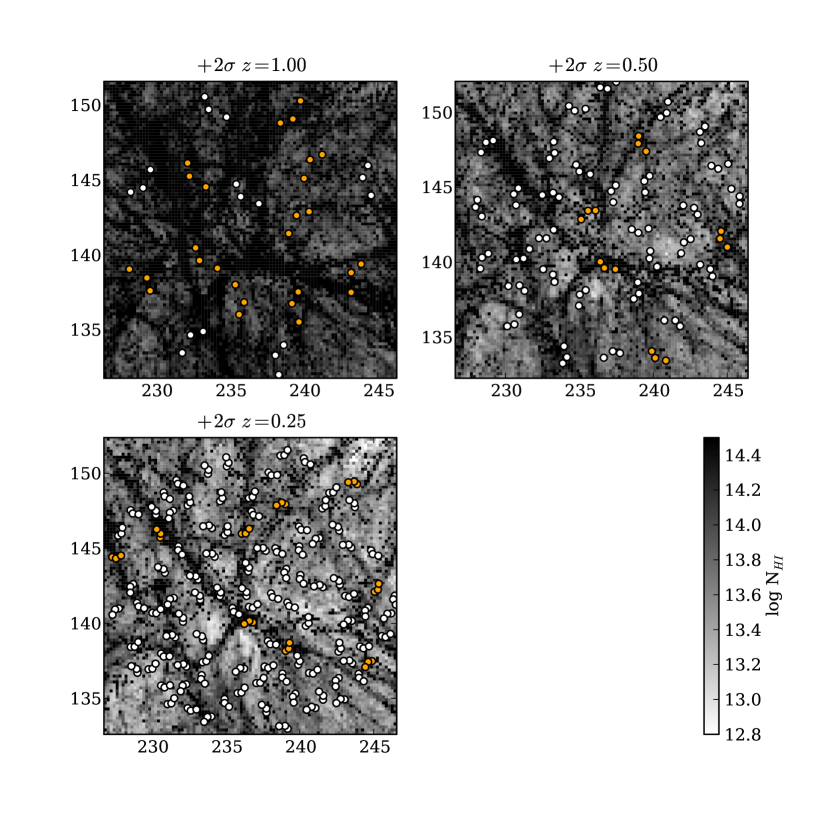
Figure 20: Similar to Figure 19, but here dots show a sample of random triple sightlines through the $+2\sigma$ density region. The sightlines denoted by darker dots contain triple LOS-galaxy groups. At $z=1$, these groups fall inside and outside filamentary structures. At $z=0.5$ and $z=0.25$, as the comoving separation of the triplets and the characteristic column density of filamentary structures drops, the groups arise in knots and filaments.

Sample sets of sightlines generated through the $+2\sigma$ region are shown in Figure 20. Even though we try to minimise sampling the same structures multiple times, inevitably this will occur to some degree, and so the Poisson errors on the number of groups detected in our simulation are probably an underestimate of the true error.

5.3 Simulated absorber properties

Once we generate sightlines, we must calculate the absorption properties of the gas along each sightline. To do this we use the program specwizard written by Joop Schaye, Craig M. Booth and Tom Theuns. specwizard finds the contributions from gas to the optical depth along a sightline though the simulation using the method described in Theuns et al. (1998). Tables generated with cloudy (Ferland, 1997), assuming an ionising background from (Haardt & Madau, 1996), determine the fraction of hydrogen in the form of H i.

specwizard calculates the optical depth, $\tau$, as a function of velocity along the sightline. This optical depth can be converted to the transmission, $T$, using $T=e^{-\tau}$. We convolved the transmission with an instrumental spread function and added noise to simulate the normalised H i flux measured in observed spectra. We use a resolution FWHM of $6.6$ km s^-1, S/N$=50$ per pixel and pixel size of 3 km s^-1, thus the mock spectra have a higher S/N and resolution that the HST FOS spectra we use in the analysis. The higher resolution allows us to fit Voigt profiles to the absorption and measure the column densities and velocity widths of lines, so that we can see if there is any change in these properties inside and outside galaxy-absorber groups. We describe below how we select a subset of absorption features that would have been detected in a FOS-quality spectrum from our higher quality spectra. A wavelength scale was generated for the spectra assuming the H i absorption is produced over a small redshift range centred at the redshift of the snapshot. The continuum level of each spectrum was assumed to be equal to the largest flux value in the spectrum and calculated after convolution with the instrumental profile, but before noise is added. This mimics a continuum fitting process, which would choose the point of highest flux over a region of a few tens of Å (comparable to the length of our simulated spectra) and consider that to be the continuum level. At these low redshifts there is not a large amount of absorption in the forest, and the difference between the inferred continuum level and the true level is a few percent or less.

We fit Voigt profiles to these spectra in an automated manner using vpfit. The fitting process generates an initial guess comprising several absorption lines, then adjusts the model parameters to minimise $\chi^{2}$. After minimising $\chi^{2}$, if the $\chi^{2}$ per degree of freedom is greater than 1.1, another absorption component is added at the point of largest deviation between the model and the data, and $\chi^{2}$ is re-minimised using the new model. Absorption components can also be removed if both their column density and $b$-parameter drop below threshold values. This process is repeated until a $\chi^{2}$ per degree of freedom $\leq 1.1$ is reached, or vpfit iterates over more than thirty add/remove cycles. A large fraction of the fitted models were visually inspected and were found to fit the data adequately.

To compare to the linelists generated using the FOS spectra, we select only systems with a column density larger than $10^{13.5}$ cm^-2; this roughly corresponds to the $3\sigma$ detection limit of the FOS spectra across the three sightlines (assuming the absorption falls on the linear part of the curve of growth). This cutoff value has a more important effect than the galaxy mass cutoff on the number of groups found, as we discuss below.

Gimic was designed to simulate the transport of metals into the IGM, and a comparison between the properties of simulated metal lines and observations will be made in a future paper. However, since we believe we have removed the majority of the metal lines from our observed line list, we have not included metal transitions in the simulated spectra. If our observed line lists contain significant numbers of features that are blended with metal lines, the simulations would appear to have fewer lines or lines with smaller equivalent widths than the observations.

The fraction of H in the form of H i (and so the amount of H i absorption) is strongly dependent on the ionising background for the highly ionised IGM. The background at low redshifts is not well known, so we check the simulated spectra are consistent with observations by measuring $dN/dz$ for H i absorbers with $13.2<$ log($N_{\rm HI}$) $<14.0$. Lehner et al. (2007) give $dN/dz$ at $z<1$ found by fitting Voigt profiles to STIS spectra over the same column density range, with a resolution comparable to that used in our simulated spectra. We find $dN/dz$ using all our mock spectra, combining the estimates for each simulated region using volume weights of $1/12$, $1/6$, $1/2$, $1/6$, $1/12$ for the (-2, -1, 0, +1, +2)$\sigma$ regions (see Crain et al., 2009). The mock spectra under-predict the line density in this range at $z\sim 0$ by a factor of $\sim 2$. We corrected for this by multiplying the optical depth used to generate the mock spectra by 1.2 (see e.g. Davé et al., 1999, for a discussion on the validity of this process at low redshifts), then generating new spectra and fitting them with vpfit.

From the fitted models we selected lines that satisfied the following criteria: $b$ parameter $<100$ km s^-1, errors in $b<40$%, and error in log($N_{\rm HI}$(cm^-2)) $<0.3$. We exclude lines with large $b$ parameters because in real data such features can be introduced (or divided out) in the continuum fitting process, and so are generally excluded from line analyses. Requiring a minimum error in the $b$ parameter and log($N_{\rm HI}$) values ensures that any poorly constrained lines, that are usually heavily blended with stronger components, are not included in our line lists. Finally, we excluded lines that occur close to the edge of the high-resolution region in the simulation. Recall that each Gimic simulation consists of a smaller, high-resolution region where dark matter, baryons and gas physics are simulated, surrounded by a larger, low resolution region where only dark matter is simulated. At the division between the pure dark matter and high resolution regions, gas physics will not be simulated correctly. Excluding lines close to the high resolution region’s edge ensures that lines affected by this incorrect gas physics are not included in our simulated line list. This final requirement restricted us to a $\sim 20\times 20\times 20$ $h^{-1}$ comoving Mpc cube in the centre of each simulation.

5.4 Simulated galaxy-absorber groups

Using the galaxies and absorbers from the simulation, selected as described in the previous sections, we identify galaxy-absorber groups in the same way as we do for the real observations. We convert the size of our $8\times 10$ arcmin field to an area in comoving Mpc at each snapshot redshift (0.25, 0.5 and 1.0), and allow any galaxy within this area, centred on each simulated set of triple sightlines, to be a group member.

To check our velocity cutoffs for associating galaxies and absorbers, we measure the number of galaxy-absorber pairs as a function of the velocity offsets between galaxies and absorber. The number of pairs drops significantly at separations larger than 500 km s^-1 in all simulations except for the $+2\sigma$ region, where there are still a significant number of pairs out to 1000 km s^-1. Thus the simulations suggest a maximum velocity cut of 1000 km s^-1 is appropriate for identifying associated galaxy-absorber pairs.

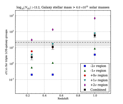
Figure 21: The number of galaxies with associated absorbers across all three sightlines (triple LOS-galaxy groups) per unit redshift in the simulations, as a function of redshift. The numbers are shown for each region, and combined across all regions, weighting each region as described in Section 5 (dark squares). The dotted line and shaded region show the observed incidence of such groups and $1\sigma$ Poisson error in the number of observed groups. The error bars show $1\sigma$ Poisson errors for the number of groups found in the simulations. The mean redshift of the observations is $\sim 0.53$.

We show the number of triple LOS-galaxy groups per unit redshift at the three snapshot redshifts in Figure 21. The values for each region are shown, and the combined value using volume weights given in Section 5.3 is also shown. The uncertainty on the value for each region is taken to be the Poisson error in the number of groups detected in sightlines through that simulated region. These are combined in quadrature with the appropriate weights to give the uncertainty in the combined value.

There are very few groups found in the low density volumes, and the vast majority of the groups are detected in the $+2\sigma$ region, even when volume weighting is taken into account. This is potentially a cause for concern – the $+2\sigma$ region was arbitrarily selected to contain a galaxy cluster at $z=0$, and so may not be truly representative of similar density regions without such a cluster. However, as long as the influence of the cluster is restricted to a relatively small percentage of the total volume analysed, it should not have a large effect on the cluster properties.

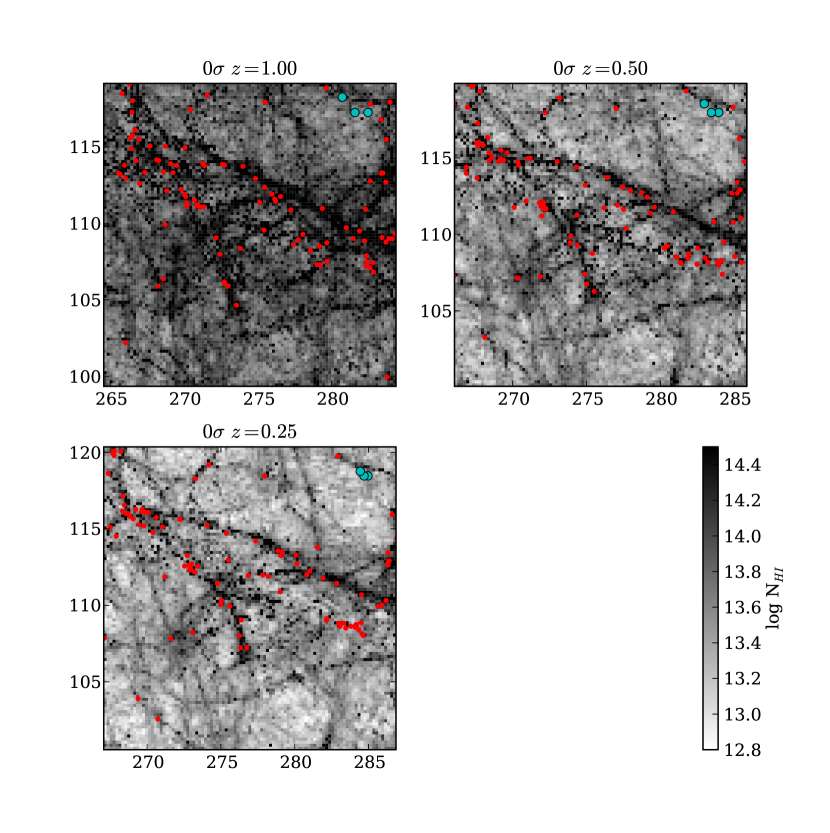
Figure 19: The X-Y positions of gas and galaxies in the mean density region of the Gimic simulation at redshifts 0.25, 0.5 and 1. Coordinates are in $h^{-1}$ comoving Mpc and refer to the original Millennium positions. The dots show galaxies with stellar mass larger than $6\times 10^{10}$ M_☉. All galaxies in the 20 $h^{-1}$ Mpc cubic region are plotted. Grayscale shows the total $N_{\rm HI}$ (cm^-2) in $200h^{-1}$ kpc $\times$ $200h^{-1}$ kpc (comoving) bins, summed along the Z axis. The group of three dots in the top right of each panel shows the configuration of triple sightlines at that redshift.

The frequency of these groups decreases with decreasing redshift. This is most likely due to the reduction in the volume fraction of gas with $N_{\rm HI}$ $>13.5$ with decreasing redshift, visible in Figure 19. Since the group finding algorithm requires at least three absorbers but only one galaxy per group, we expect it is much more sensitive to the density of absorption lines than the galaxy density. Changing the mass cuts and column density cuts used to select galaxies and absorbers confirms this expectation. Changing the mass cut has very little effect on the frequency of groups, but changing the column density cut from $10^{13.5}$ cm^-2 to $10^{13.7}$ cm^-2 changes the frequency by a factor of five.

Using our initial column density cutoff of $10^{13.5}$ cm^-2 and completeness of 20% resulted in too few groups being found at $z=0.5$ in the simulations compared to the observations, by a factor of $\sim 10$. However, if we increased the assumed completeness to 40% and decreased the column density cutoff to $10^{13.2}$ cm^-2, we found the number of simulated and observed groups was consistent (these limits are used to generate Figure 21). These values are at the extreme ranges of the expected galaxy completeness and column density sensitivities, but are not unreasonable.

One possible effect that could cause the simulations to have lower density of lines, and thus a lower frequency of groups, than the observed values is due to line blending. Close groups of weak features in the mock spectra that fall below our $N_{\rm HI}$ cutoff may still form a feature with an inferred $N_{\rm HI}$ above the cutoff after they are convolved with the instrumental spread function of the FOS spectrum. In this case we would underestimate the line density in the simulations compared to the observations. To check the magnitude of this effect, we created a set of mock spectra at a similar resolution and S/N to the FOS spectra. We detected features and fit Gaussian profiles to them in a similar manner to that used to detect lines in the real FOS spectra. Finally we selected groups of galaxies and triple absorbers using these new mock spectra. We found that the number density of groups found using the FOS-resolution mock spectra were consistent within the 1$\sigma$ errors with the number densities calculated above. Therefore we conclude that line blending does not have a significant effect on our estimate of the frequency of groups.

We are currently obtaining more galaxy redshifts in this field, and have been awarded time on COS to observe the three QSOs at high resolution; it will be interesting to see if this tension between observations and simulations persists with the new, larger data sets.

5.5 Properties of absorbers and galaxies inside and outside groups

We examined the properties of galaxies and absorbers inside the triple LOS-galaxy groups compared to galaxies outside the groups. For each combination of redshift and region density, we looked at the $b$ parameter and column density of absorbers inside groups compared to those outside groups, and the stellar and total halo masses of galaxies inside and outside groups. There are too few groups found in the $-1\sigma$ and $-2\sigma$ density regions to make a useful comparison, however we find no evidence for any difference in these properties inside and outside groups in the $0\sigma$, $+1\sigma$ and $+2\sigma$ regions. This suggests the algorithm for selecting triple LOS-galaxy groups does not preferentially select a single type of absorber or galaxy environment.

Figure 20 shows the position of our randomly-placed triple sightlines in the $+2\sigma$ simulation. The sightlines shown by darker dots contain triple LOS-galaxy groups. This is a projection of the density along the 30 Mpc simulated region, so we must take care interpreting apparent 2-d filaments as true 3-d structures. Nevertheless, at $z=1$, these groups appear to fall both inside and outside filamentary structures. At $z=0.5$ and $z=0.25$, as the comoving separation of the triplets and the characteristic column density of filamentary structures drops, the groups tend to be found in knots and filaments. We see multiple galaxies over a small redshift range in the observed triple LOS-galaxy groups($z=0.501$ and $z=0.535$), which is consistent with them arising such structures.

6 Discussion

The simulations in Figure 19 suggest two things: (1) the filaments visible over this 2-d projection maintain their geometry in comoving space through redshift. Since the comoving separation between the sightlines changes with redshift, the triple samples large scale structure on different characteristic scales at different redshifts. (2) The column density that traces the filamentary structures falls with decreasing redshift. At $z=1$, filamentary structures are traced by gas with log$N_{\rm HI}$ of 14.3, where as at $z=0$ it is traced by gas with log$N_{\rm HI}$ of about 13.5, and higher column densities now traced more collapsed, spherical structures. This implies that triple absorbers identified above a single minimum detectable equivalent width (which can be converted to a column density) will trace different kinds of structures at different redshifts – filaments and even ‘void’ regions at higher redshifts, and groups of halos at low redshift. Thus triples will tend to correspond to different kinds environments at different redshifts, depending on the combination of comoving separation and the column density sensitivity.

The excess of groups with absorbers in one or more sightlines compared to a distribution of random absorbers tells us the same thing as the nearest-neighbour test – that Ly$\alpha$ absorbers are correlated with galaxies on these scales. The significance of this excess appears to decrease as we accept absorbers with larger velocity separations from a galaxy into a group. This suggests that single absorbers are only correlated with any single galaxy on scales of $\lesssim 500$ km s^-1. This this is consistent with the results of Morris & Jannuzi (2006).

As we move to groups with absorbers in two or three sightlines, the number of groups becomes smaller. Thus the statistics are more uncertain and our interpretation is more tentative. However, we see a clear excess of galaxies with nearby absorbers in two and three sightlines at all velocity differences compared to a random absorber distribution. Interestingly, the excess of triple LOS-galaxy groups is very significant ($>99$%) for velocity separations of $750$ and $1000$ km s^-1. This suggests that the observed triple LOS-galaxy groups trace Mpc-scale structures that appear in both H i gas and galaxies. We emphasize that while a $1000$ km s^-1 separation within a single real structure appears unrealistically large if we interpret it as entirely due to the Hubble flow (a Mpc corresponds to $\sim 70$ km s^-1 at $z=0.5$), if some of the absorbers arise in winds of the magnitude described in the introduction, then such large velocity differences can still be present in a single structure less than a couple of Mpc across.

The galaxies and absorbers that make up the seven triple LOS-galaxy groups identified in the real absorbers are shown in the Figure 11 $\langle z\rangle=0.501$ and $\langle z\rangle=0.535$ panels. For both structures, there is no obvious link between any one of the galaxies and its associated absorber, in the sense that none of the absorbers are close enough to the galaxies to be caused by a ‘halo’ of gas associated with that galaxy. A more appealing explanation is that they are caused by a group of galaxies at a knot or filament of the cosmic web and its associated absorption. This absorption may be due to large diffuse IGM gas that spans the three sightlines, or more compact gas clouds closely associated with individual galaxies in the structure that have not been targeted in our spectroscopy.

In future papers we intend to present GMOS, VIMOS and DEIMOS data providing a much larger sample of galaxy redshifts in this field with a better-known selection function, along with HST Cosmic Origins Spectrograph (COS) spectra of the three QSOs. The COS spectra will resolve H i Ly$\alpha$ forest lines, detect O vi and other metal line absorbers, and allow us to measure the temperature, column density and ionisation state of the IGM.

7 Summary

We have analysed the distribution of galaxies and the intergalactic medium using three closely spaced sightlines towards background $z_{\rm em}$ $\sim 1$ QSOs.

1. We identify metal line systems in two sightlines nearby a single bright ($\sim$ L*) galaxy. The galaxy has an impact parameter of $\sim 170$ kpc from both sightlines and the absorbers are within 200 km s^-1 of the galaxy redshift. Using the galaxy’s spectrum we estimate the star formation rate and metallicity from nebular emission lines and find a SFR $>0.45$ M_☉ yr^-1 and (O/H) metallicity $\gtrsim 0.5$ solar.

2. We have identified a new probable sub-damped Ly$\alpha$ system at $z=0.557$ that shows many strong associated low-ionisation metal lines. In previous analyses that showed evidence for triple Ly$\alpha$ absorber coincidences across the three sightlines, several of these lines were assumed to be Ly$\alpha$. We show that in a re-analysis using the corrected line identifications evidence for triple coincidences remains, though at a reduced significance. Using symmetric triplet matching, there is an excess of real symmetric triples compared to random sets of absorber at the $97$% confidence level, or $99$% if a maximum velocity difference between triplet members is imposed. This is still a significant result, but less so than previous results which showed a significance $>99.99$%.

3. We show that the symmetric matching method used to detect triple coincidences across three sightlines in Petry et al can fail to detect configurations of absorbers that are consistent with a physical structure spanning the three sightlines. We present a new matching method that does detect such configurations. The significance of detected triple coincidences is reduced using this new method (94% vs 97% confidence level using symmetric matching). We speculate that symmetric matching may be more effective at differentiating between triple coincidences caused by large absorbing structures and those caused by random alignments.

4. For the six Ly$\alpha$ absorbers in QSO sightlines A and B that also show metal absorption, there is a Ly$\alpha$ absorber at a similar redshift in the adjacent sightline. The probability of this occurring by chance is $\sim 3.5$%. This is consistent with these metal systems being associated with gaseous structures seen in H i that span the two sightlines (300-400 kpc). Most absorbers with strong metal systems are not expected to arise in such large structures, but to be closely associated with a galaxy halo. We suggest that these metal absorbers may trace the halos of galaxies that are themselves embedded in a $\sim 0.5$ Mpc absorbing H i structure.

5. We measured the velocity separations between galaxies and their nearest-neighbour absorber in velocity space for all three sightlines. For each sightline we find a significant excess ($>99$%) of pairs with velocity separations $<200$ km s^-1 compared to a random distribution of absorbers.

6. We describe a new method for measuring associations between galaxies and absorbers across multiple close sightlines. We compare the number of galaxies with associated absorbers in one or more, two or more, and three sightlines found in the real sample to the number found in random sets of absorbers. In each case there is an excess of groups with real absorbers compared to the random absorber sets. We use this method to identify two apparent large-scale ($\sim 1-2$ Mpc) structures at $z=0.501$ and $z=0.535$ that show H i absorption across all three sightlines and are each associated with several galaxies.

7. We generate mock spectra using simulations, and examine the properties of galaxy-absorber groups that are similar to those found in the real observations. The number density of such groups in the simulations is consistent with the observations, taking into account the small sample size and the poorly-defined galaxy selection function. We test the galaxy mass (stellar and total halo mass), absorber $b$ parameter and column density for galaxies and absorbers inside and outside triple LOS-galaxy groups seen in the simulations. We find no significant difference in these properties inside and outside such groups. The simulations suggest that groups consisting of a galaxy and H i absorption in three nearby sightlines trace the filamentary large-scale structure at redshifts $z<0.5$.

Finally, we revisit the questions we posed in the introduction: our sample confirms that H i absorbers with a rest EW limit of $\sim 0.24$ Å are more likely to be found close to galaxies, consistent with the results of other surveys (Lanzetta et al., 1995; Penton et al., 2002; Morris & Jannuzi, 2006). We have found a galaxy that appears linked to metal absorption in two nearby sightlines. It is possible that the gas was enriched and ejected by the galaxy more than 2 Gyr ago. We also find evidence that galaxies are associated with absorption spanning the three sightlines.

The other questions – constraining the geometry of the absorbing gas and whether gas is preferentially associated with groups of galaxies – can be better addressed with improved spectra and a larger sample of galaxies, and so we defer their discussion to future papers.

8 Acknowledgements

We thank the referee for their helpful comments and a careful reading of the paper. NC thanks the Science and Technology Facilities Council for the rolling grant that funds his position. We thank Romeel Davé, Ben Oppenheimer, Joop Schaye, Adrian Jenkins, Sabrina Pakzad and Greg Davies for useful conversations and correspondence.

Simulations were carried out using the HPCx facility at the Edinburgh Parallel Computing Centre (EPCC) as part of the EC’s DEISA ‘Extreme Computing Initiative’, and with the Cosmology Machine at the Institute for Computational Cosmology at Durham University.

Many programs used for this analysis were written in Python using the Numpy and Scipy packages. Figures were produced using Matplotlib. The programs used are available from NC on request, or can be downloaded from an online code repository.

Our analysis used observations made with the NASA/ESA Hubble Space Telescope, obtained from the Hubble Legacy Archive, which is a collaboration between the Space Telescope Science Institute (STScI/NASA), the Space Telescope European Coordinating Facility (ST-ECF/ESA) and the Canadian Astronomy Data Centre (CADC/NRC/CSA).

Galaxy Properties
ID R.A.(J2000) Decl.(J2000) $z$ $z_{\rm err}$ R-mag B_max B_min 1 1:10:14.2 -2:20:10.2 0.0528 - 19.3 -15.7 -16.6 2 1:10:21.0 -2:21:27.1 0.1145 - 16.4 -20.5 -21.3 3 1:10:23.4 -2:19:34.8 0.1204 - 18.1 -18.9 -19.7 4 1:09:56.9 -2:20:52.5 0.1550 0.0004 18.1 -19.6 -20.4 5 1:10:13.7 -2:21:38.7 0.1817 - 19.0 -19.1 -19.9 6 1:10:13.1 -2:21:57.3 0.1820 - 19.0 -19.1 -19.8 7 1:10:00.1 -2:20:58.2 0.1905 - 18.8 -19.4 -20.1 8 1:10:06.2 -2:22:54.9 0.1905 - 19.5 -18.7 -19.5 9 1:10:18.4 -2:18:47.0 0.1971 - 19.3 -18.9 -19.7 10 1:10:24.3 -2:17:16.3 0.1973 - 17.5 -20.8 -21.5 11 1:10:30.4 -2:17:58.9 0.1995 0.0007 20.6 -17.7 -18.5 12 1:10:13.6 -2:17:58.8 0.1996 - 17.6 -20.7 -21.4 13 1:10:03.1 -2:22:33.5 0.1997 - 20.3 -18.1 -18.8 14 1:10:06.3 -2:18:36.1 0.1999 - 19.5 -18.8 -19.6 15 1:10:18.1 -2:18:16.5 0.2009 0.0014 19.1 -19.3 -20.0 16 1:10:28.1 -2:18:52.4 0.2009 0.0004 19.6 -18.7 -19.4 17 1:10:25.4 -2:20:02.2 0.2016 0.0007 17.2 -21.1 -21.8 18 1:10:26.0 -2:20:01.8 0.2020 0.0007 17.8 -20.6 -21.3 19 1:10:23.2 -2:16:49.8 0.2025 - 16.8 -21.5 -22.2 20 1:10:24.5 -2:19:38.5 0.2027 0.0004 19.4 -19.0 -19.7 21 1:10:11.0 -2:17:21.2 0.2029 - 19.1 -19.3 -20.0 22 1:10:21.4 -2:17:55.4 0.2029 - 17.5 -20.9 -21.6 23 1:10:24.2 -2:17:02.0 0.2029 - 18.3 -20.1 -20.8 24 1:10:23.2 -2:17:38.8 0.2032 0.0005 20.3 -18.1 -18.8 25 1:10:03.8 -2:23:34.1 0.2033 - 19.4 -19.0 -19.7 26 1:10:16.7 -2:23:02.6 0.2033 - 20.0 -18.4 -19.1 27 1:10:16.0 -2:19:36.4 0.2272 0.0007 17.7 -20.9 -21.6 28 1:10:18.1 -2:22:45.1 0.2318 - 18.0 -20.7 -21.4 29 1:10:17.2 -2:23:23.9 0.2325 - 19.6 -19.1 -19.8 30 1:10:02.1 -2:21:55.9 0.2334 0.0007 20.5 -18.2 -18.9 31 1:10:09.8 -2:23:20.6 0.2334 - 20.4 -18.4 -19.0 32 1:10:29.5 -2:20:04.9 0.2349 0.0005 19.6 -19.1 -19.8 33 1:10:29.5 -2:19:55.8 0.2366 - 18.7 -20.1 -20.8 34 1:10:18.1 -2:21:00.4 0.2367 - 19.0 -19.7 -20.4 35 1:10:04.6 -2:19:39.9 0.2373 - 19.4 -19.3 -20.0 36 1:10:09.5 -2:19:27.7 0.2380 0.0007 21.0 -17.8 -18.5 37 1:10:16.5 -2:21:37.2 0.2381 0.0007 21.5 -17.2 -17.9 38 1:10:14.5 -2:20:56.2 0.2382 0.0007 20.2 -18.5 -19.2 39 1:10:17.3 -2:21:00.9 0.2388 0.0008 19.9 -18.9 -19.6 40 1:10:02.6 -2:16:12.8 0.2421 - 19.7 -19.1 -19.7 41 1:10:19.0 -2:19:07.3 0.2616 0.0007 20.2 -18.8 -19.4 42 1:10:32.2 -2:17:55.5 0.3093 0.0007 19.5 -20.1 -20.6 43 1:10:01.8 -2:16:53.4 0.3130 - 19.7 -19.8 -20.3 44 1:10:20.3 -2:23:36.6 0.3146 - 18.4 -21.2 -21.7 45 1:09:59.4 -2:17:56.8 0.3512 0.0007 19.9 -20.0 -20.5 46 1:10:08.3 -2:21:45.6 0.3524 0.0006 19.3 -20.6 -21.1 47 1:10:26.8 -2:20:51.3 0.4279 0.0006 19.9 -20.7 -21.0 48 1:10:13.3 -2:18:20.4 0.4283 - 19.9 -20.7 -21.0 49 1:10:07.0 -2:17:10.0 0.4292 0.0007 21.0 -19.5 -19.8 50 1:10:19.5 -2:20:15.2 0.4343 0.0005 21.4 -19.2 -19.5 51 1:10:20.8 -2:21:42.1 0.4983 0.0003 20.3 -20.7 -20.9 52 1:10:04.6 -2:17:24.6 0.5014 0.0007 19.3 -21.8 -22.0 53 1:10:03.0 -2:17:34.7 0.5021 0.0007 20.1 -21.1 -21.2 54 1:10:03.7 -2:18:45.5 0.5024 0.0007 20.8 -20.4 -20.5 55 1:10:15.4 -2:18:42.8 0.5167 0.0007 20.6 -20.7 -20.8 56 1:10:21.9 -2:19:28.4 0.5349 0.0007 20.3 -21.1 -21.2 57 1:10:23.8 -2:19:36.8 0.5351 0.0007 21.8 -19.6 -19.7 58 1:10:31.3 -2:20:15.5 0.5364 0.0010 21.0 -20.4 -20.5 59 1:10:28.7 -2:21:11.5 0.5669 0.0005 20.9 -20.7 -20.8 60 1:10:10.8 -2:18:09.9 0.6438 0.0007 20.6 -21.3 -21.4

Table 2: Properties for the galaxy sample. The columns show, from left to right: galaxy ID number, right ascension and declination (with units of hours, minutes, seconds and degrees, arcminutes, arcseconds), galaxy redshifts and $1\sigma$ redshift errors, apparent R magnitude, and maximum and minimum rest-frame absolute B magnitudes. For objects with no redshift error we assume an error of 0.0007.

QSO Properties
ID Name R.A.(J2000) Decl.(J2000) $z_{\rm em}$ R-mag A LBQS 0107-025A 01:10:13:14 -02:19:52.9 0.960 18.1 B LBQS 0107-025B 01:10:16.25 -02:18:51.0 0.956 17.4 C LBQS 0107-0232 01:10:14.43 -02:16:57.6 0.726 18.4

Table 3: The QSO properties. The columns show, from left to right: ID letter, name, right ascension and declination (with units of hours, minutes, seconds and degrees, arcminutes and arcseconds), emission redshift and R magnitude.

LBQS 0107-0125A GHRS G140L
ID Wavelength(Å) EW_obs (Å) FWHM S_σ Identification $z_{\rm abs}$ 1 $1226.53\pm 0.33$ $1.26\pm 0.54$ $1.80\pm 0.97$ 6.12 - - 2 $1258.54\pm 0.19$ $1.09\pm 0.28$ $1.73\pm 0.48$ 14.30 - - 3 $1260.30\pm 0.16$ $0.73\pm 0.25$ $1.23\pm 0.35$ 9.61 Si ii 1260/Ly$\beta$ 0.0000/0.2286 4 $1265.50\pm 0.09$ $0.43\pm 0.11$ $0.80\pm 0.23$ 5.79 Ly$\beta$ 0.234 5 $1279.39\pm 0.15$ $0.53\pm 0.14$ $1.22\pm 0.41$ 6.94 - - 6 $1301.41\pm 0.13$ $0.32\pm 0.10$ $0.92\pm 0.34$ 4.87 O i 1302 0.0000 7 $1310.02\pm 1.78$ $0.67\pm 1.57$ $4.69$ 9.47 - - 8 $1334.53\pm 0.15$ $0.68\pm 0.13$ $1.63\pm 0.38$ 9.53 C ii 1334 0.0000 9 $1355.44\pm 0.18$ $0.94\pm 0.20$ $2.02\pm 0.56$ 11.88 - - 10 $1375.08\pm 0.27$ $0.36\pm 0.15$ $1.47\pm 0.77$ 5.38 - - 11 $1393.58\pm 0.12$ $0.34\pm 0.11$ $0.80\pm 0.32$ 4.11 Si iv 1393 0.0000 12 $1491.20\pm 0.30$ $1.39\pm 0.42$ $2.26\pm 0.86$ 8.60 - - 13 $1493.50\pm 0.15$ $0.82\pm 0.25$ $1.03\pm 0.37$ 4.85 Ly$\alpha$ 0.2286 14 $1500.44\pm 0.32$ $1.51\pm 0.51$ $2.45\pm 1.07$ 10.37 Ly$\alpha$ 0.234 15 $1504.52\pm 0.09$ $0.64\pm 0.16$ $0.80\pm 0.24$ 4.99 - -

Table 4: Detected lines in the GHRS G140L combined spectrum. The columns show, from left to right: line ID number, wavelength and $1\sigma$ error, observed equivalent width and $1\sigma$ error of a fitted Gaussian, FWHM and $1\sigma$ error of the fitted Gaussian, detection significance, line identification and redshift, if applicable. The wavelengths, observed equivalent widths and detection significances are from Petry et al. (2006).

LBQS 0107-0125B GHRS G140L
ID Wavelength(Å) EW_obs (Å) FWHM (Å) S_σ Identification $z_{\rm abs}$ 1 $1260.26\pm 0.17$ $0.74\pm 0.15$ $1.77\pm 0.43$ 9.11 Si ii 1260 $-0.0001$ 2 $1266.42\pm 0.22$ $0.66\pm 0.19$ $1.68\pm 0.61$ 8.37 O vi 1031 0.2273 3 $1274.16\pm 0.13$ $0.30\pm 0.10$ $0.86\pm 0.34$ 4.13 O vi 1037 0.2273 4 $1280.00\pm 0.15$ $0.33\pm 0.10$ $1.10\pm 0.41$ 5.30 - - 5 $1301.93\pm 0.11$ $0.60\pm 0.11$ $1.45\pm 0.33$ 12.52 O i 1302 $-0.0002$ 6 $1312.49\pm 0.15$ $0.26\pm 0.08$ $1.07\pm 0.42$ 5.27 Ly-5 0.3993 7 $1323.44\pm 0.10$ $0.22\pm 0.06$ $0.76\pm 0.26$ 4.49 - - 8 $1329.24\pm 0.08$ $0.50\pm 0.08$ $1.18\pm 0.22$ 9.96 Ly-4 0.3993 9 $1334.66\pm 0.10$ $0.82\pm 0.09$ $1.86\pm 0.25$ 16.80 C ii 1334 0.0001 10 $1356.06\pm 0.12$ $0.51\pm 0.10$ $1.44\pm 0.34$ 10.03 - - 11 $1361.26\pm 0.19$ $1.05\pm 0.17$ $2.79\pm 0.56$ 19.78 Ly$\gamma$ 0.3993 12 $1366.95\pm 0.14$ $0.27\pm 0.08$ $1.09\pm 0.36$ 5.38 - - 13 $1381.48\pm 0.12$ $0.36\pm 0.08$ $1.16\pm 0.30$ 7.10 - - 14 $1393.54\pm 0.19$ $0.38\pm 0.11$ $1.43\pm 0.50$ 7.03 Si iv 1393 $-0.0002$ 15 $1403.60\pm 0.09$ $0.67\pm 0.09$ $1.39\pm 0.24$ 11.37 - - 16 $1435.29\pm 0.10$ $0.42\pm 0.10$ $0.96\pm 0.27$ 6.11 Ly$\beta$ 0.3993 17 $1458.91\pm 0.07$ $0.54\pm 0.11$ $0.78\pm 0.19$ 5.91 Ly$\gamma$?/Ly$\alpha$? 0.5012/0.2001 18 $1462.24\pm 0.08$ $1.15\pm 0.14$ $1.39\pm 0.20$ 12.85 - - 19 $1492.06\pm 0.43$ $1.24\pm 0.45$ $3.44\pm 1.60$ 13.90 Ly$\alpha$ 0.2273

Table 5: Detected lines in the GHRS G140L combined spectrum of LBQS 0107-025B. See Table 4 for a description of each column.

LBQS 0107-0125A FOS G190H
ID Wavelength(Å) EW_obs (Å) FWHM (Å) S_σ Identification $z_{\rm abs}$ 1 $1637.49\pm 0.25$ $0.55\pm 0.18$ $1.58\pm 0.62$ 4.27 C ii 1334 0.2272 2 $1671.28\pm 0.13$ $0.88\pm 0.11$ $2.09\pm 0.31$ 11.30 Al ii 1670/Ly$\gamma$ 0.0000/0.7188 3 $1683.17\pm 0.09$ $0.81\pm 0.09$ $1.54\pm 0.20$ 10.74 - - 4 $1701.30\pm 0.16$ $0.61\pm 0.09$ $2.15\pm 0.39$ 9.64 Ly$\alpha$ 0.3995 5 $1721.69\pm 0.13$ $0.38\pm 0.08$ $1.24\pm 0.31$ 5.41 - - 6 $1727.48\pm 0.38$ $0.46\pm 0.12$ $2.87\pm 0.92$ 7.07 - - 7 $1738.09\pm 0.08$ $0.79\pm 0.07$ $1.70\pm 0.18$ 13.84 Ly$\gamma$/Ly-7 0.7865/0.8766 8 $1746.32\pm 0.10$ $0.16\pm 0.05$ $0.73\pm 0.25$ 2.95 Ly-6 0.8766 9 $1759.87\pm 0.16$ $0.39\pm 0.07$ $1.78\pm 0.39$ 7.40 Ly-5 0.8766 10 $1763.23\pm 0.09$ $0.83\pm 0.09$ $1.87\pm 0.23$ 13.52 Ly$\beta$ 0.7188 11 $1773.33\pm 0.13$ $0.42\pm 0.06$ $1.76\pm 0.32$ 8.79 Ly$\beta$ 0.7286 12 $1782.15\pm 0.08$ $0.60\pm 0.06$ $1.72\pm 0.21$ 12.82 Ly-4 0.8766 13 $1808.65\pm 0.15$ $0.52\pm 0.07$ $2.32\pm 0.36$ 11.46 - - 14 $1824.96\pm 0.04$ $1.82\pm 0.06$ $2.42\pm 0.10$ 40.36 Ly$\gamma$/Ly$\alpha$ 0.8766/0.5012 15 $1832.63\pm 0.11$ $0.57\pm 0.06$ $1.99\pm 0.26$ 12.81 Ly$\beta$ 0.7865 16 $1853.54\pm 0.22$ $0.21\pm 0.06$ $1.68\pm 0.55$ 4.78 - - 17 $1867.12\pm 0.03$ $2.60\pm 0.06$ $2.56\pm 0.07$ 54.57 - - 18 $1877.42\pm 0.14$ $0.14\pm 0.04$ $0.97\pm 0.34$ 3.27 - - 19 $1893.49\pm 0.07$ $0.77\pm 0.07$ $1.69\pm 0.19$ 18.23 - - 20 $1899.97\pm 0.41$ $0.86\pm 0.20$ $3.83\pm 0.97$ 19.97 C iv 1548 0.2272 21 $1903.04\pm 0.21$ $0.44\pm 0.17$ $1.98\pm 0.47$ 10.34 C iv 1550 0.2272 22 $1911.51\pm 0.12$ $0.25\pm 0.04$ $1.41\pm 0.29$ 6.72 - - 23 $1921.19\pm 0.11$ $0.67\pm 0.06$ $2.51\pm 0.27$ 18.68 - - 24 $1924.78\pm 0.05$ $0.80\pm 0.05$ $1.70\pm 0.11$ 23.11 Ly$\beta$ 0.8766 25 $1928.64\pm 0.19$ $0.25\pm 0.05$ $1.89\pm 0.50$ 7.24 - - 26 $1947.43\pm 0.07$ $0.10\pm 0.03$ $0.59\pm 0.27$ 2.75 - - 27 $1952.16\pm 0.10$ $0.11\pm 0.03$ $0.68\pm 0.24$ 3.07 - - 28 $1955.37\pm 0.10$ $0.30\pm 0.04$ $1.41\pm 0.24$ 8.01 Ly$\beta$ 0.907 29 $1976.50\pm 0.18$ $0.32\pm 0.05$ $2.16\pm 0.42$ 9.23 Ly$\beta$? 0.926 30 $1985.65\pm 0.13$ $0.29\pm 0.06$ $1.38\pm 0.31$ 8.64 - - 31 $1987.40\pm 0.14$ $0.23\pm 0.06$ $1.26\pm 0.34$ 6.92 - - 32 $1994.20\pm 0.07$ $0.47\pm 0.05$ $1.49\pm 0.18$ 14.83 C iv 1548? 0.2881 33 $1998.14\pm 0.11$ $0.21\pm 0.04$ $1.33\pm 0.27$ 6.64 C iv 1550? 0.2881 34 $2007.02\pm 0.07$ $0.32\pm 0.03$ $1.26\pm 0.16$ 14.42 Ly$\beta$ 0.957 35 $2015.66\pm 0.07$ $1.34\pm 0.05$ $4.29\pm 0.18$ 83.34 - - 36 $2022.43\pm 0.11$ $0.29\pm 0.09$ $1.64\pm 0.29$ 21.33 - - 37 $2025.66\pm 0.17$ $1.13\pm 0.22$ $3.99\pm 0.86$ 82.36 - - 38 $2028.98\pm 0.25$ $0.30\pm 0.14$ $2.18\pm 0.51$ 20.34 - - 39 $2034.10\pm 0.35$ $0.10\pm 0.04$ $1.92\pm 0.94$ 5.88 - - 40 $2036.60\pm 0.20$ $0.12\pm 0.04$ $1.38\pm 0.49$ 6.43 - - 41 $2041.44\pm 0.04$ $0.41\pm 0.03$ $1.31\pm 0.11$ 19.16 - - 42 $2054.27\pm 0.05$ $0.42\pm 0.03$ $1.50\pm 0.13$ 16.26 - - 43 $2059.89\pm 0.10$ $0.22\pm 0.03$ $1.38\pm 0.23$ 7.89 - - 44 $2073.69\pm 0.12$ $0.19\pm 0.03$ $1.39\pm 0.29$ 6.36 - - 45 $2082.10\pm 0.11$ $0.18\pm 0.03$ $1.25\pm 0.26$ 5.78 - - 46 $2089.48\pm 0.03$ $1.59\pm 0.04$ $2.31\pm 0.07$ 48.99 Ly$\alpha$ 0.7188 47 $2101.39\pm 0.02$ $1.24\pm 0.03$ $1.79\pm 0.05$ 38.72 Ly$\alpha$ 0.7286 48 $2122.79\pm 0.13$ $0.17\pm 0.03$ $1.43\pm 0.32$ 6.32 - - 49 $2131.56\pm 0.19$ $0.12\pm 0.03$ $1.39\pm 0.47$ 4.39 - - 50 $2146.95\pm 0.16$ $0.10\pm 0.03$ $1.07\pm 0.38$ 3.59 - - 51 $2166.83\pm 0.15$ $0.22\pm 0.04$ $1.88\pm 0.37$ 8.30 C iv 1548 0.3995 52 $2171.74\pm 0.03$ $1.18\pm 0.03$ $1.94\pm 0.06$ 44.57 Ly$\alpha$ 0.7865 53 $2187.61\pm 0.16$ $0.29\pm 0.04$ $2.25\pm 0.43$ 11.17 - - 54 $2196.86\pm 0.10$ $0.19\pm 0.03$ $1.29\pm 0.23$ 7.52 - - 55 $2240.78\pm 0.07$ $0.27\pm 0.03$ $1.41\pm 0.18$ 10.90 - - 56 $2246.33\pm 0.04$ $0.47\pm 0.03$ $1.34\pm 0.09$ 19.01 - - 57 $2251.63\pm 0.07$ $0.23\pm 0.03$ $1.27\pm 0.18$ 9.40 N i 1200 0.8766 58 $2262.96\pm 0.35$ $0.33\pm 0.06$ $3.89\pm 0.95$ 13.79 - - 59 $2271.83\pm 0.06$ $0.39\pm 0.03$ $1.52\pm 0.13$ 15.38 - - 60 $2281.30\pm 0.02$ $1.18\pm 0.03$ $1.71\pm 0.04$ 51.35 Ly$\alpha$ 0.8766 61 $2288.84\pm 0.12$ $0.08\pm 0.02$ $0.88\pm 0.29$ 3.54 - - 62 $2297.18\pm 0.04$ $0.39\pm 0.03$ $1.32\pm 0.10$ 16.89 - - 63 $2308.66\pm 0.05$ $0.36\pm 0.03$ $1.16\pm 0.12$ 12.49 - -

Table 6: Detected lines in the FOS G190H combined spectrum of LBQS 0107-025A. See Table 4 for a description of each column.

LBQS 0107-0125B FOS G190H
ID Wavelength(Å) EW_obs (Å) FWHM (Å) S_σ Identification $z_{\rm abs}$ 1 $1637.82\pm 0.08$ $0.51\pm 0.14$ $0.55\pm 0.20$ 2.34 C ii 1334 0.2273 2 $1671.19\pm 0.13$ $0.82\pm 0.15$ $1.55\pm 0.33$ 6.53 Al ii 1670/Ly$\gamma$ 0.0000,0.7183 3 $1680.16\pm 0.15$ $0.37\pm 0.12$ $1.00\pm 0.39$ 3.23 - - 4 $1701.06\pm 0.07$ $1.28\pm 0.12$ $1.69\pm 0.19$ 12.42 Ly$\alpha$ 0.3993 5 $1717.51\pm 0.25$ $0.62\pm 0.16$ $1.99\pm 0.60$ 5.57 - - 6 $1738.05\pm 0.16$ $0.32\pm 0.10$ $1.11\pm 0.39$ 3.57 Ly$\gamma$ 0.7874 7 $1746.62\pm 0.06$ $0.40\pm 0.07$ $0.74\pm 0.16$ 4.49 - - 8 $1759.89\pm 0.17$ $0.55\pm 0.13$ $1.56\pm 0.41$ 6.77 - - 9 $1762.53\pm 0.10$ $1.44\pm 0.16$ $2.03\pm 0.28$ 14.08 Ly$\beta$ 0.7183 10 $1784.15\pm 0.77$ $0.79\pm 0.34$ $4.13\pm 1.99$ 10.67 - - 11 $1823.58\pm 0.09$ $1.50\pm 0.11$ $2.66\pm 0.23$ 20.90 Ly$\alpha$ 0.499 12 $1844.60\pm 0.07$ $0.68\pm 0.07$ $1.31\pm 0.17$ 9.61 - - 13 $1852.68\pm 0.12$ $0.42\pm 0.08$ $1.28\pm 0.29$ 6.02 - - 14 $1855.65\pm 0.10$ $1.19\pm 0.11$ $2.32\pm 0.25$ 16.79 Ly$\beta$ 0.8094 15 $1866.73\pm 0.10$ $1.05\pm 0.11$ $2.09\pm 0.25$ 13.14 - - 16 $1919.41\pm 0.34$ $0.60\pm 0.12$ $3.56\pm 0.83$ 10.05 - - 17 $1924.62\pm 0.08$ $0.93\pm 0.08$ $2.04\pm 0.21$ 16.25 Ly$\beta$ 0.8763 18 $1950.21\pm 0.21$ $0.34\pm 0.08$ $1.78\pm 0.51$ 5.63 Si iv 1393 0.3993 19 $1956.40\pm 0.17$ $0.51\pm 0.10$ $1.96\pm 0.45$ 7.97 Ly$\beta$ 0.9065 20 $1971.91\pm 0.15$ $0.42\pm 0.08$ $1.72\pm 0.38$ 7.24 - - 21 $1997.16\pm 0.34$ $0.37\pm 0.10$ $2.72\pm 0.93$ 7.15 - - 22 $2044.48\pm 0.15$ $0.10\pm 0.03$ $0.40\pm 0.63$ 2.16 - - 23 $2048.84\pm 0.23$ $0.17\pm 0.06$ $1.42\pm 0.55$ 3.76 - - 24 $2054.50\pm 0.12$ $0.32\pm 0.05$ $1.44\pm 0.29$ 6.88 - - 25 $2064.73\pm 0.38$ $0.38\pm 0.11$ $3.07\pm 1.11$ 7.83 - - 26 $2083.57\pm 0.10$ $0.60\pm 0.06$ $2.02\pm 0.25$ 13.31 - - 27 $2088.83\pm 0.03$ $1.42\pm 0.05$ $1.81\pm 0.08$ 31.87 Ly$\alpha$ 0.7183 28 $2097.15\pm 1.13$ $0.35\pm 0.19$ $5.76\pm 4.18$ 8.11 - - 29 $2101.69\pm 0.15$ $0.20\pm 0.05$ $1.23\pm 0.37$ 4.47 - - 30 $2125.45\pm 0.22$ $0.22\pm 0.06$ $1.66\pm 0.57$ 4.81 - - 31 $2166.32\pm 0.10$ $0.30\pm 0.05$ $1.22\pm 0.23$ 6.80 C iv 1548 0.3993 32 $2170.02\pm 0.16$ $0.24\pm 0.06$ $1.42\pm 0.39$ 5.52 C iv 1550 0.3993 33 $2172.83\pm 0.07$ $0.75\pm 0.06$ $1.89\pm 0.19$ 17.19 Ly$\alpha$ 0.7874 34 $2185.55\pm 0.17$ $0.32\pm 0.06$ $1.88\pm 0.42$ 7.33 - - 35 $2199.64\pm 0.03$ $1.59\pm 0.05$ $2.00\pm 0.08$ 37.62 Ly$\alpha$ 0.8094 36 $2210.67\pm 0.13$ $0.23\pm 0.05$ $1.25\pm 0.31$ 5.26 - - 37 $2215.33\pm 0.49$ $0.24\pm 0.08$ $3.10\pm 1.18$ 5.76 - - 38 $2226.93\pm 0.09$ $0.42\pm 0.05$ $1.47\pm 0.21$ 9.99 - - 39 $2230.35\pm 0.11$ $0.34\pm 0.05$ $1.48\pm 0.26$ 8.17 - - 40 $2246.48\pm 0.26$ $0.26\pm 0.06$ $2.14\pm 0.64$ 6.37 - - 41 $2280.94\pm 0.03$ $1.08\pm 0.04$ $1.71\pm 0.08$ 29.45 Ly$\alpha$ 0.8763 42 $2297.60\pm 0.08$ $0.25\pm 0.04$ $1.09\pm 0.20$ 6.67 - -

Table 7: Detected lines in the FOS G190H combined spectrum of LBQS 0107-025B. See Table 4 for a description of each column.

LBQS 0107-0232 FOS G190H
ID Wavelength(Å) EW_obs (Å) FWHM (Å) S_σ Identification $z_{\rm abs}$ 1 $1656.72\pm 0.19$ $1.02\pm 0.31$ $1.39\pm 0.50$ 4.24 - - 2 $1670.43\pm 0.14$ $0.71\pm 0.17$ $1.20\pm 0.33$ 4.65 Al ii 1670 0.000 3 $1677.88\pm 0.30$ $1.64\pm 0.34$ $3.30\pm 0.86$ 12.34 - - 4 $1702.02\pm 0.28$ $1.34\pm 0.22$ $3.68\pm 0.78$ 14.63 Ly$\alpha$ 0.4001 5 $1732.50\pm 0.34$ $0.85\pm 0.23$ $2.63\pm 0.89$ 5.99 Ly$\beta$ 0.689 6 $1736.11\pm 0.18$ $1.65\pm 0.24$ $2.72\pm 0.48$ 11.29 - - 7 $1744.17\pm 0.55$ $0.73\pm 0.32$ $2.90\pm 1.57$ 6.17 - - 8 $1746.91\pm 0.22$ $0.65\pm 0.25$ $1.58\pm 0.48$ 6.06 - - 9 $1754.24\pm 0.16$ $1.08\pm 0.14$ $2.72\pm 0.43$ 12.77 - - 10 $1761.39\pm 0.10$ $0.53\pm 0.26$ $1.16\pm 0.35$ 7.71 Ly$\beta$ 0.7174 11 $1763.62\pm 0.68$ $0.77\pm 0.34$ $3.35\pm 1.70$ 12.55 - - 12 $1781.29\pm 0.89$ $0.54\pm 0.29$ $3.36\pm 1.50$ 13.30 Fe ii 1143 0.5569 13 $1783.14\pm 0.13$ $0.32\pm 0.25$ $1.35\pm 0.52$ 7.98 Fe ii 1144 0.5569 14 $1796.23\pm 0.20$ $0.26\pm 0.07$ $1.50\pm 0.49$ 4.12 - - 15 $1807.05\pm 0.37$ $0.62\pm 0.15$ $3.24\pm 0.95$ 6.63 - - 16 $1822.39\pm 0.14$ $0.51\pm 0.10$ $1.53\pm 0.36$ 4.94 - - 17 $1853.41\pm 0.09$ $0.79\pm 0.09$ $1.64\pm 0.22$ 7.83 Si ii 1190 0.5569 18 $1857.74\pm 0.09$ $0.72\pm 0.10$ $1.49\pm 0.24$ 6.65 Si ii 1193 0.5569 19 $1864.76\pm 0.12$ $1.58\pm 0.14$ $2.70\pm 0.28$ 13.02 - - 20 $1878.49\pm 0.07$ $1.76\pm 0.10$ $2.36\pm 0.17$ 16.81 Si iii 1206 0.5569 21 $1892.65\pm 0.07$ $4.75\pm 0.16$ $4.28\pm 0.18$ 55.70 Ly$\alpha$ 0.5569 22 $1918.61\pm 0.07$ $1.17\pm 0.09$ $1.86\pm 0.17$ 16.09 - - 23 $1962.31\pm 0.06$ $1.33\pm 0.09$ $1.94\pm 0.16$ 19.03 Si ii 1260 0.5569 24 $1971.14\pm 0.14$ $0.92\pm 0.11$ $2.50\pm 0.37$ 12.83 - - 25 $2003.89\pm 0.08$ $1.11\pm 0.10$ $2.03\pm 0.21$ 20.70 - - 26 $2027.25\pm 0.07$ $0.61\pm 0.07$ $1.20\pm 0.16$ 11.46 O i 1302 0.5569 27 $2045.29\pm 0.57$ $0.39\pm 0.26$ $1.83\pm 1.00$ 8.95 - - 28 $2046.95\pm 0.38$ $0.36\pm 0.25$ $1.48\pm 0.58$ 8.51 - - 29 $2053.70\pm 0.04$ $1.19\pm 0.05$ $1.77\pm 0.09$ 30.91 Ly$\alpha$ 0.689 30 $2067.00\pm 0.16$ $0.35\pm 0.06$ $2.12\pm 0.39$ 12.03 - - 31 $2077.75\pm 0.06$ $1.43\pm 0.10$ $1.89\pm 0.12$ 66.47 C ii 1334 0.5569 32 $2079.65\pm 0.17$ $0.39\pm 0.10$ $1.58\pm 0.31$ 19.73 - - 33 $2087.85\pm 0.02$ $2.16\pm 0.03$ $2.53\pm 0.04$ 164.89 Ly$\alpha$ 0.7174 34 $2092.54\pm 0.29$ $0.05\pm 0.02$ $1.31\pm 0.68$ 5.67 - - 35 $2113.12\pm 0.12$ $0.20\pm 0.03$ $1.42\pm 0.28$ 9.35 - - 36 $2137.71\pm 0.08$ $0.18\pm 0.03$ $1.04\pm 0.19$ 8.48 - - 37 $2263.61\pm 0.25$ $0.27\pm 0.07$ $2.15\pm 0.64$ 6.23 - -

Table 8: Detected lines in the FOS G190H combined spectrum of LBQS 0107-0232 (QSO C). See Table 4 for a description of each column.

LBQS 0107-0125A FOS G270H
ID Wavelength(Å) EW_obs (Å) FWHM (Å) S_σ Identification $z_{\rm abs}$ 1 $2247.19\pm 0.20$ $0.39\pm 0.08$ $1.88\pm 0.47$ 5.31 - - 2 $2251.98\pm 0.22$ $0.36\pm 0.08$ $1.92\pm 0.53$ 5.01 N i 1200 0.8769 3 $2272.78\pm 0.21$ $0.37\pm 0.08$ $1.95\pm 0.51$ 5.25 - - 4 $2281.72\pm 0.06$ $1.39\pm 0.08$ $2.21\pm 0.15$ 18.87 Ly$\alpha$ 0.8769 5 $2297.30\pm 0.17$ $0.35\pm 0.07$ $1.79\pm 0.41$ 5.66 - - 6 $2308.96\pm 0.18$ $0.34\pm 0.07$ $1.86\pm 0.43$ 5.86 - - 7 $2318.24\pm 0.06$ $1.21\pm 0.07$ $2.34\pm 0.15$ 21.69 Ly$\alpha$ 0.907 8 $2342.76\pm 0.06$ $1.58\pm 0.06$ $3.45\pm 0.15$ 39.88 Ly$\alpha$ 0.926 9 $2361.46\pm 0.06$ $0.49\pm 0.03$ $1.72\pm 0.13$ 21.48 - - 10 $2370.48\pm 0.09$ $0.30\pm 0.03$ $1.90\pm 0.22$ 17.45 - - 11 $2374.96\pm 0.10$ $0.17\pm 0.02$ $1.38\pm 0.23$ 11.61 - - 12 $2379.06\pm 0.03$ $0.83\pm 0.02$ $2.04\pm 0.07$ 66.83 Ly$\alpha$ 0.957 13 $2382.87\pm 0.05$ $0.50\pm 0.16$ $1.59\pm 0.20$ 40.65 Fe ii 2382 0.0000 14 $2384.81\pm 0.86$ $0.31\pm 0.17$ $3.30\pm 1.49$ 23.24 - - 15 $2389.70\pm 0.06$ $0.49\pm 0.03$ $2.11\pm 0.16$ 30.08 - - 16 $2396.46\pm 0.24$ $0.13\pm 0.03$ $1.97\pm 0.57$ 6.70 Si iv 1393 0.7194 17 $2411.81\pm 0.19$ $0.16\pm 0.04$ $1.68\pm 0.45$ 5.39 Si iv 1402 0.7194 18 $2586.76\pm 0.22$ $0.66\pm 0.09$ $3.58\pm 0.55$ 6.94 Fe ii 2586 0.0000 19 $2600.38\pm 0.09$ $0.51\pm 0.06$ $1.73\pm 0.23$ 5.16 Fe ii 2600 0.0000 20 $2796.37\pm 0.07$ $0.77\pm 0.06$ $1.95\pm 0.18$ 6.88 Mg ii 2796 0.0000 21 $2803.58\pm 0.07$ $0.65\pm 0.06$ $1.79\pm 0.18$ 5.76 Mg ii 2803 0.0000

Table 9: Detected lines in the FOS G270H combined spectrum of LBQS 0107-025A. See Table 4 for a description of each column.

LBQS 0107-0125B FOS G270H
ID Wavelength(Å) EW_obs (Å) FWHM (Å) S_σ Identification $z_{\rm abs}$ 1 $2246.72\pm 0.23$ $0.22\pm 0.06$ $1.86\pm 0.56$ 4.66 - - 2 $2281.30\pm 0.05$ $1.33\pm 0.06$ $2.38\pm 0.12$ 28.49 Ly$\alpha$ 0.8766 3 $2298.37\pm 0.20$ $0.19\pm 0.05$ $1.69\pm 0.47$ 4.70 - - 4 $2319.05\pm 0.04$ $1.01\pm 0.04$ $2.05\pm 0.10$ 26.27 Ly$\alpha$ 0.907 5 $2342.12\pm 0.18$ $0.28\pm 0.08$ $1.67\pm 0.38$ 8.43 - - 6 $2344.52\pm 0.22$ $0.48\pm 0.09$ $2.54\pm 0.50$ 15.07 Fe ii 2344 0.0000 7 $2349.38\pm 0.19$ $0.19\pm 0.04$ $1.97\pm 0.48$ 6.02 - - 8 $2374.84\pm 0.08$ $0.20\pm 0.02$ $1.39\pm 0.20$ 8.39 Fe ii 2374 0.0000 9 $2383.23\pm 0.05$ $0.67\pm 0.03$ $2.14\pm 0.11$ 25.09 Fe ii 2382 0.0000 10 $2510.88\pm 0.28$ $0.15\pm 0.05$ $1.97\pm 0.69$ 4.11 - - 11 $2587.18\pm 0.11$ $0.41\pm 0.05$ $2.06\pm 0.27$ 11.01 Fe ii 2586 0.0000 12 $2600.63\pm 0.07$ $0.53\pm 0.04$ $1.89\pm 0.17$ 14.69 Fe ii 2600 0.0000 13 $2796.64\pm 0.04$ $0.91\pm 0.04$ $1.99\pm 0.10$ 24.49 Mg ii 2796 0.0000 14 $2803.92\pm 0.05$ $0.72\pm 0.04$ $1.78\pm 0.11$ 19.65 Mg ii 2803 0.0000 15 $2853.53\pm 0.20$ $0.19\pm 0.04$ $1.86\pm 0.49$ 5.12 Mg i  2853 0.0000

Table 10: Detected lines in the FOS G270H combined spectrum of LBQS 0107-025B. See Table 4 for a description of each column.

Members of Triple Absorber Groups
sightline A sightline B sightline C $\Delta v_{\rm max}$ $\Delta v_{\rm max}$ Largest $\Delta v$ Triple LOS- ID REW (Å) ID REW (Å) ID REW (Å) Sym. 200 500 (km s^-1) gal. group? 3 $0.59\pm 0.07$ 3 $0.27\pm 0.09$ 3 $1.19\pm 0.25$ y n n 944 n 4 $0.44\pm 0.06$ 4 $0.91\pm 0.09$ 4 $0.96\pm 0.16$ y y y 169 n 14 $1.21\pm 0.04$ 11 $1.00\pm 0.07$ 16 $0.34\pm 0.07$ y n y 422 y 17 $1.69\pm 0.04$ 15 $0.68\pm 0.07$ 19 $1.03\pm 0.09$ y n y 379 y 23 $0.42\pm 0.04$ 16 $0.38\pm 0.08$ 22 $0.74\pm 0.06$ y n y 402 n 42 $0.25\pm 0.02$ 24 $0.19\pm 0.03$ 29 $0.70\pm 0.03$ y y y 117 n 45 $0.11\pm 0.02$ 26 $0.35\pm 0.04$ 32 $0.23\pm 0.06$ y n y 565 n 46 $0.93\pm 0.02$ 27 $0.83\pm 0.03$ 33 $1.26\pm 0.02$ y y y 234 n

Table 11: Absorbers that are members of symmetric triples, or triple absorber groups found using a $\Delta v_{\rm max}=200$ or $500$ km s^-1. The columns show the ID number from Tables 5, 6 or 7, the rest equivalent width and $1\sigma$ error for absorbers in each sightline; whether the triple was found using symmetric matching, whether it is found using the group matching algorithm with $\Delta v_{\rm max}=200$ and 500 km s^-1, the maximum velocity difference between any two triple members, and whether the absorbers are also members of a triple LOS-galaxy group (described in Section 4.3).

Metal Line systems
LOS $z_{\rm abs}$ Identification Wavelength(Å) EW_obs (Å) Comments A 0.2286 Ly$\alpha$ $1493.50\pm 0.15$ $0.82\pm 0.25$ - A 0.2272 C ii 1334? $1637.49\pm 0.25$ $0.55\pm 0.18$ S/N poor A 0.2272 C iv 1548 $1899.97\pm 0.41$ $0.86\pm 0.20$ - A 0.2272 C iv 1550 $1903.04\pm 0.21$ $0.44\pm 0.17$ - B 0.2273 O vi 1031? $1265.82\pm 0.22$ $0.66\pm 0.19$ S/N poor B 0.2273 O vi 1037? $1273.56\pm 0.13$ $0.30\pm 0.10$ S/N poor B 0.2273 Ly$\alpha$ $1491.46\pm 0.43$ $1.24\pm 0.45$ - B 0.2273 C ii 1334 $1637.82\pm 0.08$ $0.51\pm 0.14$ S/N poor A 0.2881 C iv 1548? $1994.20\pm 0.07$ $0.47\pm 0.05$ No coverage of Ly$\alpha$ A 0.2881 C iv 1550? $1998.14\pm 0.11$ $0.21\pm 0.04$ No coverage of Ly$\alpha$ A 0.3995 Ly$\alpha$ $1701.30\pm 0.16$ $0.61\pm 0.09$ - A 0.3995 C iv 1548 $2166.83\pm 0.15$ $0.22\pm 0.04$ C iv 1550 blended with Ly$\alpha$ B 0.3993 Ly-5 $1311.89\pm 0.15$ $0.26\pm 0.08$ - B 0.3993 Ly-4 $1328.64\pm 0.08$ $0.50\pm 0.08$ - B 0.3993 Ly$\gamma$ $1360.66\pm 0.19$ $1.05\pm 0.17$ - B 0.3993 Ly$\beta$ $1434.69\pm 0.10$ $0.42\pm 0.10$ - B 0.3993 Ly$\alpha$ $1701.06\pm 0.07$ $1.28\pm 0.12$ Lyman limit system B 0.3993 Si iv 1393 $1950.21\pm 0.21$ $0.34\pm 0.08$ Si iv 1402 blended with Ly$\alpha$ B 0.3993 C iv 1548 $2166.32\pm 0.10$ $0.30\pm 0.05$ - B 0.3993 C iv 1550 $2170.02\pm 0.16$ $0.24\pm 0.06$ - C 0.4001 Ly$\alpha$ $1702.02\pm 0.28$ $1.34\pm 0.22$ - A 0.5576 Ly$\alpha$ $1893.49\pm 0.07$ $0.77\pm 0.07$ - C 0.5569 Fe ii 1143 $1781.29\pm 0.89$ $0.54\pm 0.29$ Blended with Ly$\alpha$? C 0.5569 Fe ii 1144 $1783.14\pm 0.13$ $0.32\pm 0.25$ Blended with Ly$\alpha$? C 0.5569 Si ii 1190 $1853.41\pm 0.09$ $0.79\pm 0.09$ - C 0.5569 Si ii 1193 $1857.74\pm 0.09$ $0.72\pm 0.10$ - C 0.5569 Si iii 1206 $1878.49\pm 0.07$ $1.76\pm 0.10$ - C 0.5569 Ly$\alpha$ $1892.65\pm 0.07$ $4.75\pm 0.16$ Probable sub-DLA C 0.5569 Si ii 1260 $1962.31\pm 0.06$ $1.33\pm 0.09$ - C 0.5569 O i 1302 $2027.25\pm 0.07$ $0.61\pm 0.07$ - C 0.5569 C ii 1334 $2077.75\pm 0.06$ $1.43\pm 0.10$ - A 0.7188 Ly$\beta$ $1763.23\pm 0.09$ $0.83\pm 0.09$ - A 0.7188 Ly$\alpha$ $2089.48\pm 0.03$ $1.59\pm 0.04$ - A 0.7194 Si iv 1393 $2396.46\pm 0.24$ $0.13\pm 0.03$ Outside Ly$\alpha$ forest A 0.7194 Si iv 1402 $2411.81\pm 0.19$ $0.16\pm 0.04$ Outside Ly$\alpha$ forest B 0.7183 Ly$\beta$ $1762.53\pm 0.10$ $1.44\pm 0.16$ - B 0.7183 Ly$\alpha$ $2088.83\pm 0.03$ $1.42\pm 0.05$ - A 0.8766 N i 1200 $2251.63\pm 0.07$ $0.23\pm 0.03$ - A 0.8766 Ly-6 $1746.32\pm 0.10$ $0.16\pm 0.05$ - A 0.8766 Ly-5 $1759.87\pm 0.16$ $0.39\pm 0.07$ - A 0.8766 Ly-4 $1782.15\pm 0.08$ $0.60\pm 0.06$ - A 0.8766 Ly$\beta$ $1924.78\pm 0.05$ $0.80\pm 0.05$ - A 0.8766 Ly$\alpha$ $2281.30\pm 0.02$ $1.18\pm 0.03$ - B 0.8763 Ly$\beta$ $1924.62\pm 0.08$ $0.93\pm 0.08$ - B 0.8763 Ly$\alpha$ $2280.94\pm 0.03$ $1.08\pm 0.04$ -

Table 12: Absorption systems that have associated metal lines. H i absorbers with a similar redshift as metal line systems in adjacent sightlines are also shown. The columns show, from left to right: sightline where the line is seen; redshift; line identification; observed wavelength and $1\sigma$ error; observed equivalent width and $1\sigma$ error; and finally any comments about the line. Lines are grouped by redshift. Identifications ending in a question mark are uncertain.

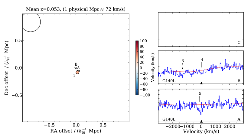
Figure 11: Galaxies and absorbers near a given redshift. Left panel: Galaxy positions relative to the three sightlines. The area of the galaxy symbol is proportional to the galaxy’s luminosity. The open circle in the top left hand corner shows the size of an L* galaxy for comparison. Galaxies are coloured by their velocity offset, and their numbers from Table 2 are shown. If there is any H i Ly$\alpha$ absorption within 1000 km s^-1 of the zero velocity position it is shown by an inverted triangle. The area of the triangle is proprtional to the summed Ly$\alpha$ rest equivalent width. If no Ly$\alpha$ absorption is detected within this range, the position of the sightline is shown by a plus sign. Right panels: Portions of the QSO spectra corresponding to H i Ly$\alpha$ near the galaxies in the left panel. Our fitted continua are also shown. Flux units are arbitrary. The tick marks indicate line positions – solid ticks are Ly$\alpha$ or unidentified lines, dotted ticks are lines that have been identified as something other than Ly$\alpha$. Line numbers from Tables 4 to 10 are shown above the tick marks. Triangles in the right panels show the velocity offsets for galaxies; filled triangles denote galaxies also shown in the left panel.

Figure. 11 — continued.

Figure. 11 — continued.

Figure. 11 — continued.

Figure. 11 — continued.

Figure. 11 — continued.

Figure. 11 — continued. Circles in the right panels show the positions of C iv and an O vi system in the A and B spectra.

Figure. 11 — continued.

Figure. 11 — continued.

Figure. 11 — continued.

Figure. 11 — continued.

Figure. 11 — continued.

Figure. 11 — continued.

Figure. 11 — continued.

Figure. 11 — continued.

Figure. 11 — continued.

Figure. 11 — continued. The position of the probable sub-DLA in sightline C with strong low ionisation metal lines is shown by a circle in the right-hand top panel.

Figure. 11 — continued.

Figure 13: H$\delta$_A and D(4000) values for the $z=0.2272$ galaxy (grey cross) overlayed on a reproduction of Figure 6 from (Kauffmann et al., 2003). Triangles represent regions where 95% of model galaxies have at least 5 percent of their stellar mass made up of stars produced in bursts of star formation over the last two Gyr. Open triangles represent galaxies where the most recent burst event began $<0.1$ Gyr ago; filled triangles correspond to galaxies where the most recent burst began $>0.1$ Gyr ago. Squares show regions where 95% of models have no stars produced in bursts of star formation over the last two Gyr. Crosses are other regions described by the model galaxies.

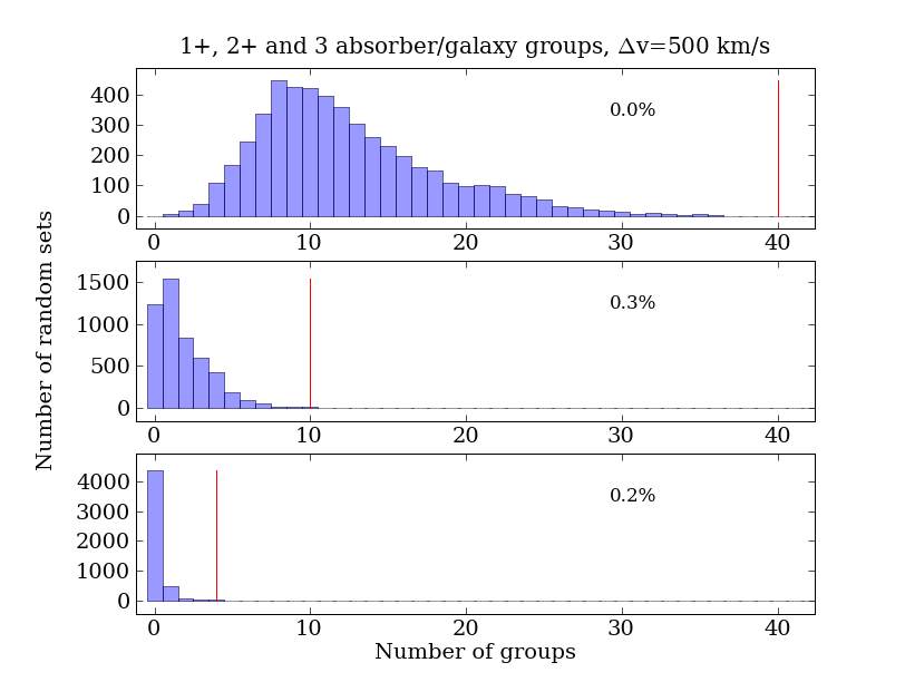
Figure 16: As for Figure 15, but using a maximum velocity difference of 500 km s^-1.

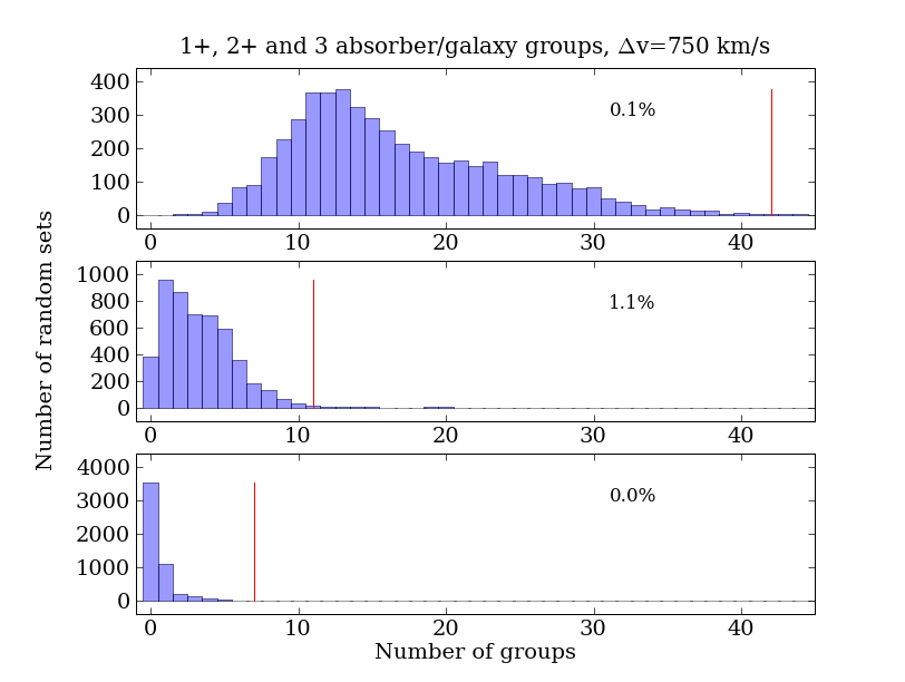
Figure 17: As for Figure 15, but using a maximum velocity difference of 750 km s^-1.

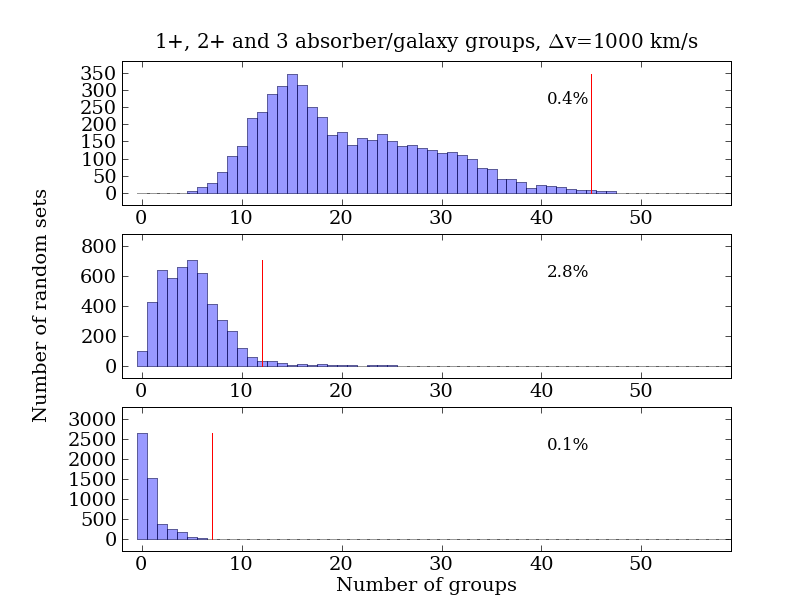
Figure 18: As for Figure 15, but using a maximum velocity difference of 1000 km s^-1.

Appendix A Method for generating random absorber sets

We generate a single random set of Ly$\alpha$ absorbers for one sightline in the following way. We draw the number of random absorbers in a set for a given sightline from a Poisson distribution with mean equal to the number of real Ly$\alpha$ absorbers in the sightline. We then generate the individual random absorbers one at a time. Each absorber is given a random wavelength between the minimum and maximum observed wavelengths in that sightline, with a rest equivalent width drawn from the exponential distribution observed in the FOS spectra in the HST Quasar absorption line key project (Weymann et al., 1998). The minimum wavelengths were lower cutoff wavelengths for the GHRS (sightlines A and B) or FOS (sightline C) wavelength settings. The maximum wavelength was taken to be 3500 km s^-1 bluewards of the QSO emission redshift to match the cutoff applied to the observations. An absorber is discarded if it falls at a wavelength where there is no spectral coverage between the GHRS and FOS spectra, its observed equivalent width is too low to be detected at its observed wavelength, or it falls within 2 Å of an existing absorber in the sightline. We calculate the minimum detectable equivalent width as a function of wavelength by fitting a low-order polynomial through the detection significances of each line given in Petry et al. (2006). We checked that our combined spectra and errors were consistent with these detection levels. Any line with detection significance less than $3\sigma$ was discarded. We discarded lines within 2 Å of existing lines because such coincidences would be fitted by a single absorption feature in the real spectra. This process is repeated until we reach the number of random absorbers for this set drawn from the Poisson distribution.

Using this method we build one thousand random sets for each sightline. We note that instead of assigning lines a random wavelength, we could have drawn their redshift from the observed line distribution; $\ell(z)\propto(1+z)^{\gamma}$. However, given the weak dependence of this term on redshift at redshifts less than one ($\gamma\lesssim 0.4$), this will have a minor effect on the line distribution. For the purposes of comparing absorbers with galaxies, our method is conservative in the sense that we will see slightly more random lines at lower redshifts compared to a $(1+z)^{0.4}$ distribution. At lower redshifts there is large overlap with the galaxy distribution, thus correcting for this effect would result in an increase in the significance of any correlation between Ly$\alpha$ lines and galaxies.

Appendix B Description of galaxy-absorber groups

This section describes the remaining galaxy-absorber groups shown in Figure 11.

$z=0.053$

This is an $\sim 0.03$ L* galaxy very close to the A (25 kpc) and B (90 kpc) sightlines. Two Ly$\alpha$ lines in both sightlines are within 200 km s^-1 of the galaxy velocity. The line at a smaller impact parameter has a larger equivalent width. This is consistent with H i gas surrounding the galaxy with a high covering factor out to $\sim$65 kpc.

$z=0.115$

A single bright galaxy 350 kpc / 400 kpc from the A/B sightlines. Ly$\alpha$ lines appear within 200 km s^-1 of the galaxy in both sightlines.

$z=0.120$

A single $0.7$ L* galaxy is 280 kpc from sightline B and 380 kpc from sightline A. A weak Ly$\alpha$ line within 100 km s^-1 appears in sightline B; no line is seen in sightline A.

$z=0.155$

A single galaxy 780 kpc from sightline A and 970 kpc from sightline B. Ly$\alpha$ absorption is seen only in sightline B within 200 km s^-1 of the galaxy. The A spectrum is noisy, but consistent with weaker Ly$\alpha$ at the same velocity as the line seen in the B spectrum.

$z=0.190$

Three pairs of galaxies are seen close to this redshift. One is very close ($130$ kpc) to the B sightline. No significant Ly$\alpha$ absorption is seen within 1000 km s^-1 of any of these galaxies. However, there is absorption in the B spectrum about 500 km s^-1 from both the lower redshift pair and the higher redshift pair, which has been identified as a transition other than Ly$\alpha$. It is possible that this is blended with Ly$\alpha$ absorption.

$z=0.202$

A group of 16 galaxies spread over $\sim 1000$ km s^-1, generally distributed around sightline B. One is 175 kpc from sightline B and several have a luminosity of a few times L*. A strong Ly$\alpha$ line is seen in spectrum B, but no line is seen in spectrum A. There is also a feature in spectrum B at -700 km s^-1 that we identified as Ly$\gamma$ from a higher redshift absorber that may be blended with Ly$\alpha$.

$z=0.233$

A group of five galaxies south of sightlines A and B. Absorption is seen within 500 km s^-1 of the mean galaxy velocity in sightline B. No absorption is seen in sightline A.

$z=0.238$

A group of seven galaxies close to sightline A. The galaxy with the smallest impact parameters is 280 kpc from sightline A and 500 kpc from sightline B. Absorption is seen in sightline A, but not in sightline B.

$z=0.242$

A single galaxy 1.2 Mpc from sightlines A and B. No associated absorption is seen within 1000 km s^-1.

$z=0.352$

At this redshift Ly$\alpha$ coverage begins for the spectrum of the third sightline. There are two galaxies, the smallest separation for a QSO sightline is 900 kpc from sightline A. No Ly$\alpha$ absorption is seen within 1000 km s^-1, but spectra B and C are noisy in this region.

$z=0.428$

Three galaxies are seen, one within 730 kpc of sightlines A and C, and 420 kpc of sightline B. Absorption is seen within 1000 km s^-1 of the galaxies in sightlines A and C, but not in sightline B.

$z=0.434$

A single galaxy about 800 kpc from sightlines A and B. Absorption is seen in the B and C spectra. No Ly$\alpha$ absorption is seen in spectrum A, although there is an absorber identified with Ly-6 from a higher-redshift system.

$z=0.501$

A group of three galaxies 1.6 Mpc from all three sightlines, and a fourth galaxy 1.5 Mpc from sightlines A and B. The galaxy with the smallest impact parameter is 1.4 Mpc from sightline C. Strong absorption is seen in sightline A; weaker Ly$\alpha$ absorption is seen in sightlines B and C. The absorption represents an absorber triplet (as defined in Section 3), and this triplet forms four triple LOS-galaxy groups (defined in Section 4.3) with the four nearby galaxies.

$z=0.517$

A single galaxy very close (130 kpc) to sightline B. Ly$\alpha$ is seen in sightline B only.

$z=0.535$

Three galaxies, one of which is 900 kpc from sightline B. Absorption is seen within 200 km/s in all three sightlines. The absorption represents a triplet (as defined in Section 3) and it forms three triple LOS-galaxy groups (defined in Section 4.3) with the three nearby galaxies.

$z=0.567$

A single galaxy 2.4 Mpc from sightline B. No Ly$\alpha$ absorption within 1000 km s^-1 is seen in any of the spectra. We do not observe a galaxy linked with the sub-DLA absorption in sightline C at $z=0.5569$.

$z=0.644$

A single galaxy 1 Mpc from sightlines B and C. Ly$\alpha$ is seen within 200 km s^-1 of the galaxy position in sightlines B and A.

References

- Adelberger et al. (2005) Adelberger K. L., Shapley A. E., Steidel C. C., Pettini M., Erb D. K., Reddy N. A., 2005, ApJ, 629, 636
- Asplund et al. (2004) Asplund M., Grevesse N., Sauval A. J., Allende Prieto C., Kiselman D., 2004, A&A, 417, 751
- Bahcall et al. (1991) Bahcall J. N., Jannuzi B. T., Schneider D. P., Hartig G. F., Bohlin R., Junkkarinen V., 1991, ApJ, 377, L5+
- Bahcall & Spitzer (1969) Bahcall J. N., Spitzer L., 1969, Astrophysical Journal, 156, L63
- Balogh et al. (1999) Balogh M. L., Morris S. L., Yee H. K. C., Carlberg R. G., Ellingson E., 1999, ApJ, 527, 54
- Bechtold et al. (1994) Bechtold J., Crotts A. P. S., Duncan R. C., Fang Y., 1994, ApJ, 437, L83
- Bergeron & Boisse (1991) Bergeron J., Boisse P., 1991, A&A, 243, 344
- Bertin & Arnouts (1996) Bertin E., Arnouts S., 1996, A&AS, 117, 393
- Boksenberg & Sargent (1978) Boksenberg A., Sargent W. L. W., 1978, Astrophysical Journal, 220, 42
- Bruzual A. (1983) Bruzual A. G., 1983, ApJ, 273, 105
- Chen et al. (2005) Chen H.-W., Kennicutt Jr. R. C., Rauch M., 2005, ApJ, 620, 703
- Chen et al. (2001) Chen H.-W., Lanzetta K. M., Webb J. K., 2001, ApJ, 556, 158
- Chen et al. (1998) Chen H.-W., Lanzetta K. M., Webb J. K., Barcons X., 1998, ApJ, 498, 77
- Chen et al. (2001) Chen H.-W., Lanzetta K. M., Webb J. K., Barcons X., 2001, ApJ, 559, 654
- Chen et al. (2005) Chen H.-W., Prochaska J. X., Weiner B. J., Mulchaey J. S., Williger G. M., 2005, ApJ, 629, L25
- Churchill et al. (2000) Churchill C. W., Mellon R. R., Charlton J. C., Jannuzi B. T., Kirhakos S., Steidel C. C., Schneider D. P., 2000, ApJ, 543, 577
- Colberg et al. (2005) Colberg J. M., Krughoff K. S., Connolly A. J., 2005, MNRAS, 359, 272
- Crain et al. (2009) Crain R. A., Theuns T., Dalla Vecchia C., Eke V. R., Frenk C. S., Jenkins A., Kay S. T., Peacock J. A., Pearce F. R., Schaye J., Springel V., Thomas P. A., White S. D. M., Wiersma R. P. C., 2009, ArXiv e-prints
- Dalla Vecchia & Schaye (2008) Dalla Vecchia C., Schaye J., 2008, MNRAS, 387, 1431
- Davé et al. (1999) Davé R., Hernquist L., Katz N., Weinberg D. H., 1999, ApJ, 511, 521
- Dinshaw et al. (1995) Dinshaw N., Foltz C. B., Impey C. D., Weymann R. J., Morris S. L., 1995, Nat, 373, 223
- Dinshaw et al. (1997) Dinshaw N., Weymann R. J., Impey C. D., Foltz C. B., Morris S. L., Ake T., 1997, ApJ, 491, 45
- Dolag et al. (2008) Dolag K., Borgani S., Murante G., Springel V., 2008, ArXiv e-prints, 808
- Eke et al. (2004) Eke V. R., Baugh C. M., Cole S., Frenk C. S., Norberg P., Peacock J. A., Baldry I. K., Bland-Hawthorn J., Bridges T., Cannon R., Colless M., Collins C., Couch W., Dalton G., de Propris R., Driver S. P., Efstathiou G., Ellis R. S., Glazebrook K., Jackson C., Lahav O., Lewis I., Lumsden S., Maddox S., Madgwick D., Peterson B. A., Sutherland W., Taylor K., 2004, MNRAS, 348, 866
- Faber et al. (2007) Faber S. M., Willmer C. N. A., Wolf C., Koo D. C., Weiner B. J., Newman J. A., Im M., Coil A. L., Conroy C., Cooper M. C., Davis M., Finkbeiner D. P., Gerke B. F., Gebhardt K., Groth E. J., Guhathakurta P., Harker J., Kaiser N., Kassin S., Kleinheinrich M., Konidaris N. P., Kron R. G., Lin L., Luppino G., Madgwick D. S., Meisenheimer K., Noeske K. G., Phillips A. C., Sarajedini V. L., Schiavon R. P., Simard L., Szalay A. S., Vogt N. P., Yan R., 2007, ApJ, 665, 265
- Fadda et al. (1996) Fadda D., Girardi M., Giuricin G., Mardirossian F., Mezzetti M., 1996, ApJ, 473, 670
- Ferland (1997) Ferland G., 1997, Hazy, a Brief Introduction to Cloudy. University of Kentucky, Department of Physics and Astronomy Internal Report
- Foltz et al. (1987) Foltz C. B., Chaffee Jr. F. H., Hewett P. C., MacAlpine G. M., Turnshek D. A., Weymann R. J., Anderson S. F., 1987, AJ, 94, 1423
- Franx et al. (1991) Franx M., Illingworth G., de Zeeuw T., 1991, ApJ, 383, 112
- Frenk et al. (1996) Frenk C. S., Evrard A. E., White S. D. M., Summers F. J., 1996, ApJ, 472, 460
- Gharanfoli et al. (2007) Gharanfoli S., Kulkarni V. P., Chun M. R., Takamiya M., 2007, AJ, 133, 130
- Haardt & Madau (1996) Haardt F., Madau P., 1996, ApJ, 461, 20
- Hamann (1998) Hamann F., 1998, Astrophysical Journal, 500, 798
- Heckman et al. (1990) Heckman T. M., Armus L., Miley G. K., 1990, ApJS, 74, 833
- Jenkins et al. (2005) Jenkins E. B., Bowen D. V., Tripp T. M., Sembach K. R., 2005, ApJ, 623, 767
- Kacprzak et al. (2008) Kacprzak G. G., Churchill C. W., Steidel C. C., Murphy M. T., 2008, AJ, 135, 922
- Kauffmann et al. (2003) Kauffmann G., Heckman T. M., White S. D. M., Charlot S., Tremonti C., Brinchmann J., Bruzual G., Peng E. W., Seibert M., Bernardi M., Blanton M., Brinkmann J., Castander F., Csábai I., Fukugita M., Ivezic Z., Munn J. A., Nichol R. C., Padmanabhan N., Thakar A. R., Weinberg D. H., York D., 2003, MNRAS, 341, 33
- Kennicutt (1998) Kennicutt Jr. R. C., 1998, ARA&A, 36, 189
- Kewley & Dopita (2002) Kewley L. J., Dopita M. A., 2002, ApJS, 142, 35
- Kewley et al. (2002) Kewley L. J., Geller M. J., Jansen R. A., Dopita M. A., 2002, AJ, 124, 3135
- Kroupa (2001) Kroupa P., 2001, MNRAS, 322, 231
- Lanzetta et al. (1995) Lanzetta K. M., Bowen D. V., Tytler D., Webb J. K., 1995, ApJ, 442, 538
- Le Brun et al. (1996) Le Brun V., Bergeron J., Boisse P., 1996, A&A, 306, 691
- Lehner et al. (2007) Lehner N., Savage B. D., Richter P., Sembach K. R., Tripp T. M., Wakker B. P., 2007, ApJ, 658, 680
- Morris & Jannuzi (2006) Morris S. L., Jannuzi B. T., 2006, MNRAS, 367, 1261
- Morris et al. (1993) Morris S. L., Weymann R. J., Dressler A., McCarthy P. J., Smith B. A., Terrile R. J., Giovanelli R., Irwin M., 1993, ApJ, 419, 524
- Morris et al. (1991) Morris S. L., Weymann R. J., Savage B. D., Gilliland R. L., 1991, ApJ, 377, L21
- Navarro et al. (2004) Navarro J. F., et al., 2004, MNRAS, 349, 1039
- Penton et al. (2002) Penton S. V., Stocke J. T., Shull J. M., 2002, ApJ, 565, 720
- Petry et al. (2006) Petry C. E., Impey C. D., Fenton J. L., Foltz C. B., 2006, AJ, 132, 2046
- Power et al. (2003) Power C., Navarro J. F., Jenkins A., Frenk C. S., White S. D. M., Springel V., Stadel J., Quinn T., 2003, MNRAS, 338, 14
- Prochaska et al. (2006) Prochaska J. X., O’Meara J. M., Herbert-Fort S., Burles S., Prochter G. E., Bernstein R. A., 2006, ApJ, 648, L97
- Ramella et al. (1989) Ramella M., Geller M. J., Huchra J. P., 1989, ApJ, 344, 57
- Rao et al. (2003) Rao S. M., Nestor D. B., Turnshek D. A., Lane W. M., Monier E. M., Bergeron J., 2003, ApJ, 595, 94
- Rauch & Haehnelt (1995) Rauch M., Haehnelt M. G., 1995, MNRAS, 275, L76
- Schaye (2001) Schaye J., 2001, ApJ, 559, 507
- Schaye & Dalla Vecchia (2008) Schaye J., Dalla Vecchia C., 2008, MNRAS, 383, 1210
- Scott et al. (2002) Scott J., Bechtold J., Morita M., Dobrzycki A., Kulkarni V. P., 2002, ApJ, 571, 665
- Sheth et al. (2003) Sheth R. K., Bernardi M., Schechter P. L., Burles S., Eisenstein D. J., Finkbeiner D. P., Frieman J., Lupton R. H., Schlegel D. J., Subbarao M., Shimasaku K., Bahcall N. A., Brinkmann J., Ivezić Ž., 2003, ApJ, 594, 225
- Smette et al. (1995) Smette A., Robertson J. G., Shaver P. A., Reimers D., Wisotzki L., Koehler T., 1995, A&AS, 113, 199
- Springel et al. (2005) Springel V., et al., 2005, Nat, 435, 629
- Springel et al. (2001) Springel V., White S. D. M., Tormen G., Kauffmann G., 2001, MNRAS, 328, 726
- Steidel et al. (1994) Steidel C. C., Dickinson M., Persson S. E., 1994, ApJ, 437, L75
- Stocke et al. (2004) Stocke J. T., Keeney B. A., McLin K. M., Rosenberg J. L., Weymann R. J., Giroux M. L., 2004, ApJ, 609, 94
- Stocke et al. (1995) Stocke J. T., Shull J. M., Penton S., Donahue M., Carilli C., 1995, ApJ, 451, 24
- Theuns et al. (1998) Theuns T., Leonard A., Efstathiou G., 1998, MNRAS, 297, L49
- Theuns et al. (1998) Theuns T., Leonard A., Efstathiou G., Pearce F. R., Thomas P. A., 1998, MNRAS, 301, 478
- Theuns et al. (2002) Theuns T., Viel M., Kay S., Schaye J., Carswell R. F., Tzanavaris P., 2002, ApJ, 578, L5
- Tripp et al. (1998) Tripp T. M., Lu L., Savage B. D., 1998, ApJ, 508, 200
- Wagoner (1967) Wagoner R. V., 1967, Astrophysical Journal, 149, 465
- Weymann et al. (1998) Weymann R. J., Jannuzi B. T., Lu L., Bahcall J. N., Bergeron J., Boksenberg A., Hartig G. F., Kirhakos S., Sargent W. L. W., Savage B. D., Schneider D. P., Turnshek D. A., Wolfe A. M., 1998, ApJ, 506, 1
- Wiersma et al. (2009) Wiersma R. P. C., Schaye J., Smith B. D., 2009a, MNRAS, pp 20–+
- Wiersma et al. (2009) Wiersma R. P. C., Schaye J., Theuns T., Dalla Vecchia C., Tornatore L., 2009b, ArXiv e-prints
- Wild et al. (2008) Wild V., Kauffmann G., White S., York D., Lehnert M., Heckman T., Hall P. B., Khare P., Lundgren B., Schneider D. P., vanden Berk D., 2008, Monthly Notices of the Royal Astronomical Society, 388, 227
- Wilman et al. (2007) Wilman R. J., Morris S. L., Jannuzi B. T., Davé R., Shone A. M., 2007, MNRAS, 375, 735
- Worthey & Ottaviani (1997) Worthey G., Ottaviani D. L., 1997, ApJS, 111, 377
- Young et al. (2001) Young P. A., Impey C. D., Foltz C. B., 2001, ApJ, 549, 76