Quadrupole collective states within the Bohr collective Hamiltonian

Abstract

The article reviews the general version of the Bohr collective model for the description of quadrupole collective states, including a detailed discussion the model’s kinematics. The quadrupole coordinates, momenta and angular momenta are defined and the structure of the isotropic tensor fields as functions of the tensor variables is investigated. After the comprehensive discussion of the quadrupole kinematics, the general form of the classical and quantum Bohr Hamiltonian is presented. The electric and magnetic multipole moments operators acting in the collective space are constructed and the collective sum rules are given. A discussion of the tensor structure of the collective wave functions and a review of various methods of solving the Bohr Hamiltonian eigenvalue equation are also presented. Next, the methods of derivation of the classical and quantum Bohr Hamiltonian from the microscopic many-body theory are recalled. Finally, the microscopic approach to the Bohr Hamiltonian is applied to interpret collective properties of twelve heavy even-even nuclei in the Hf-Hg region. Calculated energy levels and E2 transition probabilities are compared with experimental data.

1 Introduction

The story of the Bohr collective Hamiltonian seems to go back to 1879, long before the discovery of atomic nuclei, when Lord Rayleigh [1] showed that the time dependent coefficients, $\alpha_{\lambda\mu}(t)$, in equation

$$R(\theta,\phi;t)=R_{0}\left(1+\sum_{\lambda,\mu}\alpha_{\lambda\mu}(t)Y^{\ast}_{\lambda\mu}(\theta,\phi)\right)$$ (1.1)

of the surface of an incompressible liquid drop in the spherical coordinates $R,\theta,\phi$ play the role of normal modes of small oscillations of the surface around a spherical shape. The next milestone was the liquid drop model of an atomic nucleus [2] — an object known already at that time. It allowed Flügge [3] to apply the Rayleigh normal modes to a classical description of low-energy excitations of spherical nuclei. The model of Rayleigh and Flügge was quantized by Aage Bohr [4] who formulated in this way the quantum model of surface vibrations of spherical nuclei. It was Aage Bohr also, who introduced the concept of the intrinsic frame of reference for the quadrupole nuclear surface and replaced the variables $\alpha_{2\mu}$ by the Euler angles and parameters $\beta$ and $\gamma$ (nowadays often called the Bohr deformation parameters) which describe the surface in the intrinsic system. Afterwards, Bohr and Mottelson [5] generalized the model to vibrations and rotations of deformed nuclei. A generalization of the Bohr Hamiltonian to describe large-amplitude collective quadrupole excitations of any even-even nuclei was proposed by Belyaev [6] and Kumar and Baranger [7]. This general form of the Bohr collective Hamiltonian is sketched in Volume 2 of the Bohr-Mottelson book [8]. In the meantime several specific forms of the collective Hamiltonian intended to describe the collective excitations in nuclei of different types were proposed [9, 10, 11, 12, 13, 14]. All that belongs to the past. During the last decades of the twentieth century and in the beginning of the twenty first century, a great progress in the development of microscopic many-body theories of nuclear systems took place. However, it is still not possible for the self-consistent Hartree-Fock-Bogolyubov approach, employing single-particle degrees of freedom, to directly describe the collective phenomena in nuclei. One of the methods which can be used in order obtain such a description is the Adiabatic Time Dependent Hartree-Fock-Bogolyubov theory (ATDHFB) [6, 15, 16], which in the case of the quadrupole coordinates leads to the Bohr Hamiltonian. On the other hand, the Random Phase Approximation (RPA) (cf [17, 18] for its application to nuclear physics) is not able to explain a large amplitude collective motion because it assumes harmonicity of the excitations. The other method which can extend a microscopic approach to the collective phenomena is the Generator Coordinate Method (GCM) [19]. In its Gaussian Overlap Approximation (GOA) [20, 21] the GCM also yields the Bohr Hamiltonian [22, 23]. The integral Hill-Wheeler equation of the GCM without this approximation for all five quadrupole generator coordinates is considerably more difficult to solve [24].

It is not an intention of the present article to review all applications of the Bohr Hamiltonian used to describe the nuclear quadrupole collective excitations which have been done hitherto. Neither is the full list of publications on this subject compiled here. Rather the review focuses on the Bohr Hamiltonian itself. Section 2 contains a detailed discussion of the kinematics of the quadrupole degrees of freedom. Tensor properties of the coordinates and momenta themselves are a subject, which goes far beyond the Bohr Hamiltonian model. The discussion is based on the concept of the isotropic tensor fields presented in A. The tensor algebra and analysis allow us to investigate in section 3 the possible most general form of the Hamiltonian and other observables. Moreover, the tensor structure of the collective wave function with a definite spin is presented. In section 3 we also recall some analytically solvable examples of the Bohr Hamiltonian and we briefly review different methods of solving the eigenvalue equation of the general Hamiltonian. A specific version of the collective model is determined by several scalar functions which define the Hamiltonian and all other observables. Within the phenomenological approach to the collective model the parameters of all these scalar functions are fixed using experimental data on properties of the collective excitations. Obviously, there is another possibility, that all the necessary tensor fields, such as the collective potential, the inertial functions, the moments of charge distribution and the gyromagnetic tensors, are derived from an underlying more fundamental theory. Among others, the classical or semi-classical theories or models, such as different versions of the liquid drop model (e.g. [3, 25, 26]) or the Thomas-Fermi model [27, 28] can be used and because of such a possible classical background the Bohr Hamiltonian is usually qualified as the geometrical model. However, we focus here on the quantum methods of derivation of the Bohr Hamiltonian from a microscopic many-body theory. In section 4 the ATDHFB theory, which leads to the classical (at the intermediate stage) collective Hamiltonian, and the Generator Coordinate Method, which gives the quantum Hamiltonian directly, are recalled and their application to the collective quadrupole Bohr Hamiltonian is presented. The section ends with an example of calculations which illustrates the entire reviewed approach that leads from a microscopic theory through the Bohr Hamiltonian to the description of the collective quadrupole excitations in several even-even nuclei (¹⁷⁸Hf — ²⁰⁰Hg). Some important properties of the ATDHFB inertial functions are discussed in B.

2 Quadrupole collective coordinates

The fundamental assumption of the Bohr collective model applied to the description of the quadrupole collective states is that the dynamical variables (coordinates) form a real quadrupole electric, i.e. of the positive parity (cf A.1), tensor $\alpha_{2}^{(\mathrm{E})}$ (the superscript (E) will be omitted below). It is not necessary to give the tensor $\alpha_{2}$ a geometrical interpretation. In particular, the interpretation of $\alpha_{2}$ coming from (1.1), even if often used, is not needed. Thus, referring to the model as to the geometrical model is, in general, unjustified. Indeed, at the present time the Bohr model with some special forms of the collective Hamiltonian is formulated and treated simply as an algebraic collective model (cf e.g. [29, 30, 31]).

2.1 The laboratory coordinates

Let the covariant components $\alpha_{2\mu}$ ($\mu=-2,\,\dots,\,2$) of a tensor $\alpha_{2}$ in the laboratory system U_lab form a set of five independent dynamical variables. Although in general, it is convenient to use complex coordinates, there are, in fact, five real coordinates $a_{2\mu}\ (\mu=0,\,1,\,2)$ and $b_{2\mu}\ (\mu=1,\,2)$ which are respectively the real and imaginary parts of $\alpha_{2\mu}$ (see (2.3eizabadahaoapgprsvwaeagahaiascaeamang) for definition). The volume element in the space of these coordinates is (cf (2.3eizabadahaoapgprsvwaeagahaiascaeamann))

$$\rmd\Omega=\prod_{\mu=0}^{2}\rmd a_{2\mu}\prod_{\mu=1}^{2}\rmd b_{2\mu}.$$ (2.1)

The covariant momentum tensor and the contravariant momentum Hermitian adjoint to it (cf (2.3eizabadahaoapgprsvwaeagahaiascaeamanv) and (2.3eizabadahaoapgprsvwaeagahaiascaeamanw)) are $\hat{\pi}_{2\mu}=-\rmi\hbar\partial/\partial\alpha^{\ast}_{2\mu}$ and $\hat{\pi}_{2\mu}^{{\dagger}}=-\rmi\hbar\partial/\partial\alpha_{2\mu}$, respectively. The angular momentum vector connected with rotations in the physical three-dimensional space, expressed by the five components of the quadrupole tensor, reads (cf (2.3eizabadahaoapgprsvwaeagahaiascaeamanz))

$$\hat{L}_{1\nu}\equiv\hat{L}^{(2)}_{1\nu}=\rmi\sqrt{10}\left[\alpha_{2}\times\hat{\pi}_{2}\right]_{1\nu}.$$ (2.2)

2.2 The intrinsic coordinates

Apart from, perhaps, the case of the five-dimensional harmonic oscillator Hamiltonian [4], the laboratory coordinates are not used in practice. Usually, one introduces the system of principal axes of the tensor $\alpha_{2}$, U_in, called the intrinsic system. The orientation of U_in with respect to U_lab is given by the three Euler angles, $\varphi$, $\vartheta$, $\psi$. For given laboratory components $\alpha_{2\mu}$ the Euler angles are defined through the three implicit relations:

$$\sum_{\mu}D^{2\ast}_{\mu\pm 1}(\varphi,\vartheta,\psi)\alpha_{2\mu} = 0,$$ (2.3a)

$$\sum_{\mu}D^{2\ast}_{\mu 2}(\varphi,\vartheta,\psi)\alpha_{2\mu} = \sum_{\mu}D^{2\ast}_{\mu-2}(\varphi,\vartheta,\psi)\alpha_{2\mu}$$ (2.3b)

which imply vanishing of the following real and imaginary parts of the intrinsic components $\alpha^{(\mathrm{in})}_{2\mu^{\prime}}$ of $\alpha_{2}$:

$$a^{(\mathrm{in})}_{21}=b^{(\mathrm{in})}_{21}=b^{(\mathrm{in})}_{22}=0.$$ (2.3d)

The two remaining real parts of the intrinsic components are

$$a_{20}^{(\mathrm{in})}\equiv a_{0} = \sum_{\mu}D^{2\ast}_{\mu 0}(\varphi,\vartheta,\psi)\alpha_{2\mu},$$ (2.3ea)

$$a_{22}^{(\mathrm{in})}\equiv a_{2} = \frac{1}{\sqrt{2}}\sum_{\mu}\left(D^{2\ast}_{\mu 2}(\varphi,\vartheta,\psi)+D^{2\ast}_{\mu-2}(\varphi,\vartheta,\psi)\right)\alpha_{2\mu}.$$ (2.3eb)

These coordinates are usually parametrized by two parameters, $\beta$ and $\gamma$ ($0\leq\beta<\infty$, $-\pi\leq\gamma\leq\pi$) defined by the relations

$$a_{0}=\beta\cos{\gamma}\qquad a_{2}=\beta\sin{\gamma}.$$ (2.3ef)

The parameters $\beta$ and $\gamma$, commonly known as the Bohr deformation parameters, play the role of polar coordinates in plane $(a_{0}a_{2})$ (see figure 1). In equations (2.3a), (2.3b), (2.3ea) and (2.3eb) the Wigner functions with $\nu\neq 0$ appear in the following combinations denoted as

$$D^{2(\pm)}_{\mu\nu}(\varphi,\vartheta,\psi)=\frac{1}{\sqrt{2}}\left(D^{2}_{\mu\nu}(\varphi,\vartheta,\psi)\pm(-1)^{\nu}D^{2}_{\mu-\nu}(\varphi,\vartheta,\psi)\right)\ .$$ (2.3eg)

Relations (2.3a), (2.3b), (2.3ea) and (2.3eb) define the transformation

$$\alpha_{2\mu}(a_{0},a_{2},\varphi,\vartheta,\psi)=D^{2}_{\mu 0}(\varphi,\vartheta,\psi)a_{0}+D^{2(+)}_{\mu 2}(\varphi,\vartheta,\psi)a_{2}$$ (2.3eh)

from the intrinsic coordinates $a_{0},\,a_{2},\,\varphi,\,\vartheta,\,\psi$ to the laboratory ones — $\alpha_{2\mu}\;(\mu=-2,\,\dots,\,2)$. The Jacobian of this transformation is, up to a constant coefficient, equal to (cf [32])

$$D(a_{0},a_{2},\varphi,\vartheta,\psi)=\left|\frac{\mathrm{D}(\alpha_{2-2},\dots,\alpha_{22})}{\mathrm{D}(a_{0},a_{2},\varphi,\vartheta,\psi)}\right|=|X(a_{0},a_{2})|\sin{\vartheta}$$ (2.3eia)

$$X(a_{0},a_{2})=a_{2}(3a_{0}^{2}-a_{2}^{2})a_{2}(\sqrt{3}a_{0}+a_{2})(\sqrt{3}a_{0}-a_{2})=\beta^{3}\sin{3\gamma}.$$ (2.3eib)

The transformation (2.3ef) to the polar coordinates $\beta$ and $\gamma$ adds the factor $\beta$ to the Jacobian (2.3eib) since $\rmd a_{0}\rmd a_{2}=\beta\rmd\beta\rmd\gamma$. For values of the intrinsic coordinates for which the Jacobian is not equal to zero the transformation is invertible, meaning that the intrinsic frame can be defined. The inverse transformation is given by implicit functions of the Euler angles. The Jacobian vanishes on the three straight lines in the $(a_{0}a_{2})$ plane specified by the conditions

$$a_{x}=0\ \mathrm{or}\ \gamma=0,\pm\pi\qquad a_{y}=0\ \mathrm{or}\ \gamma=\pi/3,-2\pi/3\qquad a_{z}=0\ \mathrm{or}\ \gamma=2\pi/3,-\pi/3$$ (2.3eij)

where

$$a_{x}=-\frac{1}{2}\left(\sqrt{3}a_{0}+a_{2}\right)=\beta\sin{\gamma_{x}}\qquad a_{y}=\frac{1}{2}\left(\sqrt{3}a_{0}-a_{2}\right)=\beta\sin{\gamma_{y}}$$

$$a_{z}=a_{2}=\beta\sin{\gamma_{z}}\qquad\mathrm{and}\qquad\gamma_{x}=\gamma-2\pi/3\qquad\gamma_{y}=\gamma+2\pi/3\qquad\gamma_{z}=\gamma.$$ (2.3eik)

The lines intersect at the point $a_{0}=a_{2}=0\ (\beta=0)$ and divide the plane into six sectors as is shown in figure 1. At the boundaries of these sectors the intrinsic frame cannot be uniquely defined. The reason is that the tensor $\alpha_{2}$ is then axially symmetric (cf (2.3eizabadahaoapgprsvwaeagahaiascaeamanb)).

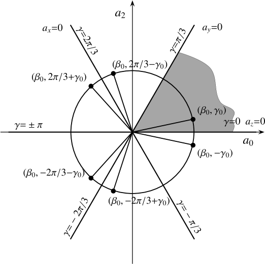
Figure 1: Three straight lines: $a_{x}=0$, $a_{y}=0$, $a_{z}=0$ (or six rays: $\gamma=0$, $\gamma=\pm\pi/3$, $\gamma=\pm 2\pi/3$, $\gamma=\pm\pi$) going through the origin of the coordinate system and dividing the $(a_{0}a_{2})$ plane into the six sectors. Each point of the polar coordinates $(\beta_{0},\gamma_{0})$ located in the sector $0\leq\gamma\leq\pi/3$ has five twin points in the remaining five sectors. All these six points of polar coordinates $(\beta_{0},\pm\gamma_{0})$, $(\beta_{0},\pm 2\pi/3\pm\gamma_{0})$, marked with full circles, are equivalent to each other. This means that any intrinsic component of a tensor field at one of these points is a linear combination with constant coefficients of the intrinsic components of the same field at any other of the remaining five points. It is therefore sufficient to consider tensor fields in one sector only. Usually, the shadowed sector, $0\leq\gamma\leq\pi/3$, is considered.

As will become clear, the appearance of the three lines, instead of only one, on which the Jacobian vanishes, reflects the fact that equations (2.3a) and (2.3b) define, in general, three mutually perpendicular axes in the three dimensional space but not their ordering (say $x,y,z$) nor their arrows. This means that the axes are defined up to a discrete group of 48 transformations O_k, $k=0,\,\dots,\,47$, changing the names and arrows of the axes. The group is the symmetry group of a cube and is denoted by O_h (cf [33]).

Traditionally, one generates all the 48 transformations ${\mathrm{O}}_{k}\in{\mathrm{O}}_{\mathrm{h}}$ by three so called Bohr’s rotations, R₁, R₂, R₃, and the inversion P (other sets of generators can also be chosen). Definitions of the Bohr’s rotations are given in table 2.2. The twenty four unimodular transformations (rotations) O_k for $k=0,\,\dots,\,23$, which are the products of the Bohr’s rotations are listed in [35] (but the numbering in [35] is different from that used in this paper). The remaining twenty four transformations can be formed by composing the unimodular ones with the inversion.

Table 1: Generators of the O_h group of transformations of the coordinate system. The index $k$ numbers the transformations. The angles $\varpi_{k}$, $\varrho_{k}$, $\varsigma_{k}$ are the Euler angles defining the orientation of the coordinate system after the transformation O_k. The coordinates $x_{k}$, $y_{k}$, $z_{k}$ define the position with respect to the transformed system.

• Transformation			The Euler angles			Coordinates
  $k$	Description	Ok	$\varpi_{k}$	$\varrho_{k}$	$\varsigma_{k}$	$x_{k}$	$y_{k}$	$z_{k}$
  ​0	Identity	E	0	0	0	$x$	$y$	$z$
  1	Bohr’s	R1	$\pi$	$\pi$	0	$x$	$-y$	$-z$
  2	rotat-	R2	0	0	$\pi/2$	$y$	$-x$	$z$
  3	ions	R3	0	$\pi/2$	$\pi/2$	$y$	$z$	$x$
  24	Inversion	P	0	0	0	$-x$	$-y$	$-z$

  The transformation rules of the tensor $\alpha_{2}$ under the O_h transformations are presented in table 2. Since the tensor $\alpha_{2}$ has the positive parity, it is insensitive to the inversion of the coordinate system. For $\alpha_{2}$ it is therefore sufficient to consider only the SO(3) group of rotations. The five-dimensional irreducible representation $D^{(2)}$ of SO(3) can be decomposed into two irreducible representations, $E$ and $F_{2}$, of the octahedral group O. These irreducible representations are identical with representations of O_h [33]. This is clear from table 2, where the transformation rules of the real and imaginary parts of $\alpha_{2\mu}$ under the Bohr’s rotations are shown. The bases of the irreducible representations $E$ and $F_{2}$ are easily identified. Clearly, $a_{20}$ and $a_{22}$ form a basis of the two-dimensional irreducible representation $E$ of O, whereas the components $-a_{21}$, $-b_{21}$, $b_{22}$ form a basis of the three-dimensional irreducible representation $F_{2}$. This makes obvious that equalities (2.3d) are invariant under the O_h transformations.

  Table 2: Transformation rules of $a_{2\mu}$ and $b_{2\mu}$ under R₁, R₂ and R₃. The real and imaginary parts of the $\alpha_{2}$ components transformed by R_k are denoted by $a_{2\mu}^{(k)}$ and $b_{2\mu}^{(k)}$. Decomposition into two irreducible representations of the group O, $E$ and $F_{2}$, is also shown.

  • 		$E$		$F_{2}$
    $k$	Ok	$a^{(k)}_{20}$	$a^{(k)}_{22}$	$a^{(k)}_{21}$	$b^{(k)}_{21}$	$b^{(k)}_{22}$
    0	E	$a_{20}$	-$a_{22}$	-$a_{21}$	-$b_{21}$	-$b_{22}$
    1	R1	$a_{20}$	-$a_{22}$	$-a_{21}$	-$b_{21}$	$-b_{22}$
    2	R2	$a_{20}$	$-a_{22}$	-$b_{21}$	$-a_{21}$	$-b_{22}$
    3	R3	$-\frac{1}{2}a_{20}+\frac{\sqrt{3}}{2}a_{22}$	$-\frac{\sqrt{3}}{2}a_{20}-\frac{1}{2}a_{22}$	$-b_{21}$	-$b_{22}$	$-a_{21}$
    24	P	$a_{20}$	-$a_{22}$	-$a_{21}$	-$b_{21}$	-$b_{22}$

  When names and arrows of the intrinsic axes are changed, intrinsic coordinates $a_{0}$, $a_{2}$ (or $\beta$, $\gamma$), $\varphi$, $\vartheta$, $\psi$ of (2.3eh) are transformed accordingly. Changes of the deformation parameters and of the orientation angles under the O transformations are given in table 3. Values of the Euler angles $\varphi_{3},\ \vartheta_{3},\ \psi_{3}$ after the circular permutation R₃ of the intrinsic axes can be found from the following equations given in [34]:

  $$\cos{\vartheta_{3}}=-\sin{\vartheta}\cos{\psi}\qquad\sin{\vartheta_{3}}\sin{\psi_{3}}=\cos{\vartheta}\qquad\cos{(\varphi_{3}-\varphi)}=\cos{\psi}\sin{\psi_{3}}.$$ (2.3eil)

  Table 3: Transformations of the Bohr deformation parameters and of the Euler angles defining the orientation of the intrinsic axes with respect to the laboratory axes under the Bohr’s rotations R_k, $k=1,2,3$, of the intrinsic coordinate system. The Euler angles $\varphi_{3}$, $\vartheta_{3}$, $\psi_{3}$ giving the orientation of the intrinsic system with axes permuted circularly can be found from equations (2.3eil).

  • Bohr’s rotation					Deformations		The Euler angles
    $k$	Ok	$\varpi_{k}$	$\varrho_{k}$	$\varsigma_{k}$	$\beta_{k}$	$\gamma_{k}$	$\varphi_{k}$	$\vartheta_{k}$	$\psi_{k}$
    0	E	0	0	0	$\beta$	-$\gamma$	$\varphi$	$\vartheta$	-$\psi$
    1	R1	$\pi$	$\pi$	0	$\beta$	-$\gamma$	$\varphi\pm\pi$	$\pi-\vartheta$	$-\psi$
    2	R2	0	0	$\pi/2$	$\beta$	$-\gamma$	$\varphi$	$\vartheta$	$\psi+\pi/2$
    3	R3	0	$\pi/2$	$\pi/2$	$\beta$	$\gamma-2\pi/3$	$\varphi_{3}$	$\vartheta_{3}$	$\psi_{3}$

  The Wigner functions of the Euler angles $\varphi_{k},\vartheta_{k},\psi_{k}$ giving the orientation of the rotated intrinsic system are related to those of the Euler angles $\varphi,\vartheta,\psi$ of the orientation of the initial intrinsic system by the following superposition formula [34]:

  $$D^{\lambda}_{\mu\nu}(\varphi_{k},\vartheta_{k},\psi_{k})=\sum_{\mu^{\prime}}D^{\lambda}_{\mu\mu^{\prime}}(\varphi,\vartheta,\psi)D^{\lambda}_{\mu^{\prime}\nu}(\varpi_{k},\varrho_{k},\varsigma_{k})$$ (2.3eim)

  where $\varpi_{k},\varrho_{k},\varsigma_{k}$ with $k=0,1,2,3$ are the Euler angles of the corresponding rotation.

  In order to present the contravariant and covariant momentum tensors as differential operators in the intrinsic variables, one should first calculate the derivatives of the intrinsic coordinates with respect to the components of the tensor $\alpha_{2}$ using relations (2.3a), (2.3b) and (2.3ea), (2.3eb). The calculation is a bit tedious. Relations (2.3a) and (2.3b), when differentiated with respect to $\alpha_{2\mu}$, yield a system of three linear equations for the derivatives of the Euler angles from which the derivatives themselves can be calculated. Useful formulae for the derivatives of the Wigner functions with respect to the Euler angles can be found in [34]. By differentiating relations (2.3ea) and (2.3eb) with respect to $\alpha_{2\mu}$ one obtains the derivatives of $a_{0}$ and $a_{2}$. The complete calculation is performed in [32]. The final result for the momentum tensor reads:

  $$\hat{\pi}_{2\mu}=-\rmi\hbar\left(D^{2}_{\mu 0}(\varphi,\vartheta,\psi)\frac{\partial}{\partial a_{0}}+D^{2(+)}_{\mu 2}(\varphi,\vartheta,\psi)\frac{\partial}{\partial a_{2}}\right)+\frac{\rmi D^{2(-)}_{\mu 2}(\varphi,\vartheta,\psi)}{2a_{z}}\hat{L}_{z}(\varphi,\vartheta,\psi)$$

  $$-\frac{\rmi D^{2(-)}_{\mu 1}(\varphi,\vartheta,\psi)}{2a_{x}}\hat{L}_{x}(\varphi,\vartheta,\psi)-\frac{D^{2(+)}_{\mu 1}(\varphi,\vartheta,\psi)}{2a_{y}}\hat{L}_{y}(\varphi,\vartheta,\psi)$$ (2.3ein)

  where $a_{x}$, $a_{y}$, $a_{z}$ are defined by (2.3eik), and

  $$\hat{L}_{x}(\varphi,\vartheta,\psi) = -\rmi\hbar\left(-\frac{\cos{\psi}}{\sin{\vartheta}}\frac{\partial}{\partial\varphi}+\sin{\psi}\frac{\partial}{\partial\vartheta}+\cot{\vartheta}\cos{\psi}\frac{\partial}{\partial\psi}\right)$$

  $$\hat{L}_{y}(\varphi,\vartheta,\psi) = -\rmi\hbar\left(\frac{\sin{\psi}}{\sin{\vartheta}}\frac{\partial}{\partial\varphi}+\cos{\psi}\frac{\partial}{\partial\vartheta}-\cot{\vartheta}\sin{\psi}\frac{\partial}{\partial\psi}\right)$$ (2.3eio)

  $$\hat{L}_{z}(\varphi,\vartheta,\psi) = -\rmi\hbar\frac{\partial}{\partial\psi}$$

  are the Cartesian intrinsic components of the angular momentum. Indeed, from (2.3eizabadahaoapgprsvwaeagahaiascaeamanz), (2.3eh) and (2.3ein) one can derive the following relations

  $$\hat{L}^{(\mathrm{in})}_{10}=\hat{L}_{z}\qquad\hat{L}^{(\mathrm{in})}_{1\pm 1}=\mp\frac{1}{\sqrt{2}}\left(\hat{L}_{x}\pm\hat{L}_{y}\right)$$ (2.3eip)

  between the laboratory and the intrinsic spherical components of the angular momentum vector:

  $$\hat{L}_{1\mu}=\sum_{\nu}D^{1}_{\mu\nu}\hat{L}^{(\mathrm{in})}_{1\nu}.$$ (2.3eiq)

  It should be remembered that the spherical intrinsic components of angular momentum fulfill the commutation relations with the sign opposite to that of (2.3eizabadahaoapgprsvwaeagahaiascaeamanac), namely

  $$[\hat{L}_{1\mu}^{(\mathrm{in})},\hat{L}_{1\nu}^{(\mathrm{in})}]=+\hbar\sqrt{2}(1\mu 1\nu|1\kappa)\hat{L}_{1\kappa}^{(\mathrm{in})}$$ (2.3eir)

  and that these components commute with the laboratory ones

  $$[\hat{L}_{1\mu}^{(\mathrm{in})},\hat{L}_{1\nu}]=0.$$ (2.3eis)

  Using the deformation parameters instead of the intrinsic components one should replace in (2.3ein) the derivatives with respect to $a_{0}$ and $a_{2}$ by the derivatives with respect to $\beta$ and $\gamma$:

  $$\frac{\partial}{\partial a_{0}}=\cos{\gamma}\frac{\partial}{\partial\beta}-\sin{\gamma}\frac{1}{\beta}\frac{\partial}{\partial{\gamma}}\qquad\frac{\partial}{\partial a_{2}}=\sin{\gamma}\frac{\partial}{\partial\beta}+\cos{\gamma}\frac{1}{\beta}\frac{\partial}{\partial{\gamma}}.$$ (2.3eit)

  It should be noticed that both the laboratory and the intrinsic components of angular momentum do not commute with the Wigner functions and that the order of $D^{2(\pm)}_{\mu\nu}$ and $\hat{L}^{(\mathrm{in})}_{1\nu}$ in (2.3ein) is essential (this is not so in (2.3eiq) — see [36]). However, it is sometimes convenient to exchange their order using the commutation relations. Doing so in the formulae for the Hermitian adjoint momentum one obtains:

  $$\hat{\pi}^{{\dagger}}_{2\mu}=-\rmi\hbar\left(\left(\frac{\partial}{\partial a_{0}}+\frac{\sqrt{3}}{2}\left(\frac{1}{a_{y}}-\frac{1}{a_{x}}\right)\right)\left(D^{2}_{\mu 0}(\varphi,\vartheta,\psi)\right)^{\ast}\right.$$

  $$+\left.\left(\frac{\partial}{\partial a_{2}}+\frac{1}{2}\left(\frac{2}{a_{z}}-\frac{1}{a_{x}}-\frac{1}{a_{y}}\right)\right)\left(D^{2(+)}_{\mu 2}(\varphi,\vartheta,\psi)\right)^{\ast}\right)-\frac{\rmi}{2a_{z}}\hat{L}_{z}(\varphi,\vartheta,\psi)\left(D^{2(-)}_{\mu 2}(\varphi,\vartheta,\psi)\right)^{\ast}$$

  $$+\frac{\rmi}{2a_{x}}\hat{L}_{x}(\varphi,\vartheta,\psi)\left(D^{2(-)}_{\mu 1}(\varphi,\vartheta,\psi)\right)^{\ast}-\frac{1}{2a_{y}}\hat{L}_{y}(\varphi,\vartheta,\psi)\left(D^{2(+)}_{\mu 1}(\varphi,\vartheta,\psi)\right)^{\ast}.$$ (2.3eiu)

  Using the deformation parameters $\beta$ and $\gamma$ one should appropriately express the derivatives and take the dependence of $a_{0}$ and $a_{2}$ on $\beta,\ \gamma$ into account. The following relations are useful to this end:

  $$\frac{\sqrt{3}}{2}\left(\frac{1}{a_{y}}-\frac{1}{a_{x}}\right)=\frac{3\sin{2\gamma}}{\beta\sin{3\gamma}}\qquad\frac{1}{2}\left(\frac{2}{a_{z}}-\frac{1}{a_{x}}-\frac{1}{a_{y}}\right)=\frac{3\cos{2\gamma}}{\beta\sin{3\gamma}}.$$ (2.3eiv)

  At the end of the discussion of the intrinsic coordinates, let them be functions of the parameter $t$ (time in the case of classical motion). The laboratory coordinates become then the functions of $t$ too. The derivatives of $\alpha_{2\mu}$ with respect to $t$ read:

  $$\dot{\alpha}_{2\mu}=\dot{a}_{0}D^{2}_{\mu 0}(\varphi,\vartheta,\psi)+\dot{a}_{2}D^{2(+)}_{\mu 2}(\varphi,\vartheta,\psi)$$

  $$-2\rmi\omega_{x}a_{x}D^{2(-)}_{\mu 1}(\varphi,\vartheta,\psi)-2\omega_{y}a_{y}D^{2(+)}_{\mu 1}(\varphi,\vartheta,\psi)+2\rmi\omega_{z}a_{z}D^{2(-)}_{\mu 2}(\varphi,\vartheta,\psi)$$ (2.3eiw)

  where

  $$\omega_{x}=\dot{\vartheta}\sin{\psi}-\dot{\varphi}\sin{\vartheta}\cos{\psi}\qquad\omega_{y}=\dot{\vartheta}\cos{\psi}+\dot{\varphi}\sin{\vartheta}\sin{\psi}\qquad\omega_{z}=\dot{\psi}+\dot{\varphi}\cos{\vartheta}$$ (2.3eix)

  play the role of the intrinsic components of the angular velocity. The derivatives $\dot{a}_{0}$ and $\dot{a}_{2}$ can be expressed by $\dot{\beta}$ and $\dot{\gamma}$:

  $$\dot{a}_{0}=\dot{\beta}\cos{\gamma}-\beta\dot{\gamma}\sin{\gamma}\qquad\dot{a}_{2}=\dot{\beta}\sin{\gamma}+\beta\dot{\gamma}\cos{\gamma}.$$ (2.3eiy)

  2.3 Functions of the coordinates

  The general rules presented in A for constructing isotropic tensor fields of a given tensor are applied here to the case of the quadrupole tensor $\alpha_{2}$. In this case one has the following five elementary tensors [37]:

  1. two quadrupole tensors

     $$\alpha_{2\mu} = \varepsilon^{(1)}_{2\mu}(\alpha_{2})$$ (2.3eiza)

     $$\sigma_{2\mu}=-\sqrt{7/2}[\alpha_{2}\times\alpha_{2}]_{2\mu} \propto \varepsilon^{(2)}_{2\mu}(\alpha_{2})$$ (2.3eizb)

  2. two scalars

     $$\sigma_{0}=(\alpha_{2}\cdot\alpha_{2}) \propto \varepsilon^{(2)}_{00}(\alpha_{2})$$ (2.3eizc)

     $$\chi_{0}=(\alpha_{2}\cdot\sigma_{2}) \propto \varepsilon^{(3)}_{00}(\alpha_{2})$$ (2.3eizd)

  3. one octupole tensor

     $$\chi_{3\mu}=\sqrt{2}[\alpha_{2}\times\sigma_{2}]_{3\mu}\propto\varepsilon^{(3)}_{3\mu}(\alpha_{2}).$$ (2.3eize)

  The elementary tensors are related to each other by the single syzygy which reads (cf [38]):

  $$\left[\chi_{3}\times\chi_{3}\right]_{6M}=\frac{\sqrt{6}}{3}\left\{2\chi_{0}\left[\alpha_{2}\times\alpha_{2}\times\alpha_{2}\right]_{6M}\right.$$

  $$\left.-3\sigma_{0}\left[\alpha_{2}\times\alpha_{2}\times\sigma_{2}\right]_{6M}+\left[\sigma_{2}\times\sigma_{2}\times\sigma_{2}\right]_{6M}\right\}.$$ (2.3eizaa)

  Since the intrinsic components $\alpha_{2\pm 1}^{(\mathrm{in})}=0$ (see (2.3a)), the only nonvanishing intrinsic components of the elementary tensors are

  $$\alpha_{20}^{(\mathrm{in})}=a_{0}=\beta\cos{\gamma}\qquad\alpha_{2\pm 2}^{(\mathrm{in})}=\frac{1}{\sqrt{2}}a_{2}=\frac{1}{\sqrt{2}}\beta\sin{\gamma}$$ (2.3eizaba)

  $$\sigma_{20}^{(\mathrm{in})}=a_{0}^{2}-a_{2}^{2}=\beta^{2}\cos{2\gamma}\qquad\sigma_{2\pm 2}^{(\mathrm{in})}=-\sqrt{2}a_{0}a_{2}=-\frac{1}{\sqrt{2}}\beta^{2}\sin{2\gamma}$$ (2.3eizabb)

  $$\chi_{32}^{(\mathrm{in})}=-\chi_{3-2}^{(\mathrm{in})}=\frac{1}{\sqrt{2}}a_{2}(3a_{0}^{2}-a_{2}^{2})=\frac{1}{\sqrt{2}}\beta^{3}\sin{3\gamma}.$$ (2.3eizabc)

  The scalars $\sigma_{0}$ and $\chi_{0}$ are the following functions of $a_{0}$ and $a_{2}$, or $\beta$ and $\gamma$:

  $$\sigma_{0}=a_{0}^{2}+a_{2}^{2}=\beta^{2}\qquad\chi_{0}=a_{0}(a_{0}^{2}-3a_{2}^{2})=\beta^{3}\cos{3\gamma}.$$ (2.3eizabac)

  Scalar functions depending on $\sigma_{0}$ and $\chi_{0}$ can be treated as functions of $\beta$ and $\zeta=\cos{3\gamma}$. The fundamental tensors of a given even rank $2L$ ($L=0,\,\dots$) are built up from elementary tensors $\alpha_{2}$ and $\sigma_{2}$ as follows:

  $$\tau_{k\,2L}\equiv\tau_{2L}^{(n)}=\left[\underbrace{\alpha_{2}\times\cdots\times\alpha_{2}}_{2L-n}\times\underbrace{\sigma_{2}\times\cdots\times\sigma_{2}}_{n-L}\right]_{2L}$$ (2.3eizabada)

  for $$k=1,\,\dots,L+1 n=L,\,\dots,2L k n \alpha_{2} n=L+k-1 2L+3 L=1 \chi_{3}$$ (), where stands for the tensor consecutive number and — for its order in (). To construct the fundamental tensors of an odd rank (the tensor with does not exist) one aligns the even rank tensors (2.3eizabada) with the single elementary tensor (see (2.3)):

  $$\tau_{k\,2L+3}\equiv\tau_{2L+3}^{(n+3)}=\left[\underbrace{\alpha_{2}\times\cdots\times\alpha_{2}}_{2L-n}\times\underbrace{\sigma_{2}\times\cdots\times\sigma_{2}}_{n-L}\times\chi_{3}\right]_{2L+3}.$$ (2.3eizabadb)

  The ranges of $l$ and $n$ do not change. Obviously, for the fundamental tensors, only the intrinsic components with even magnetic numbers are nonvanishing. An analytic formula for the intrinsic components of the fundamental tensors created by aligning several $\alpha_{2}$’s alone is known [39, 40]. It reads:

  $$\tau_{1\,2l\,2m}^{(\mathrm{in})}=\left[\underbrace{\alpha_{2}\times\cdots\times\alpha_{2}}_{l}\right]_{2l\,2m}^{(\mathrm{in})}=\beta^{l}t_{2l\,2m}(\gamma)$$ (2.3eizabadae)

  where

  $$t_{2l\,2m}(\gamma)=\sqrt{\frac{(2l+2m)!(2l-2m)!}{(4l)!}}{l\choose m}\left(\sqrt{6}\right)^{l-m}\left(\cos{\gamma}\right)^{l-m}\left(\frac{1}{\sqrt{2}}\sin{\gamma}\right)^{m}$$

  $$\times{}_{2}F_{1}\left(-\frac{l-m}{2},-\frac{l-m-1}{2};m+1;\frac{1}{3}\tan^{2}{\gamma}\right)$$ (2.3eizabadaf)

  with ${}_{2}F_{1}$ being the hypergeometric function [41]. Then, comparing (2.3eizabb) with (2.3eizaba) one finds that

  $$\tau_{l+1\,2l\,2m}^{(\mathrm{in})}=\left[\underbrace{\sigma_{2}\times\cdots\times\sigma_{2}}_{l}\right]_{2l\,2m}^{(\mathrm{in})}=\beta^{2l}t_{2l\,2m}(-2\gamma).$$ (2.3eizabadag)

  The fundamental tensor with a given even rank $2L$ and the number $k=n+1\ (n=0,\ \dots,L)$ is created by aligning the tensors (2.3eizabadae) and (2.3eizabadag) with ranks $2l=2L-2n$ and $2l=2n$, respectively. To form the fundamental tensor of an odd rank, the third one, namely $\chi_{3}$ of (2.3eizabc) should be aligned. For further use, it is convenient to introduce the ‘dimensionless’ intrinsic components of the fundamental tensors which depend only on $\gamma$:

  $$t_{n+1\,2L\,2K}(\gamma)=\frac{1}{\beta^{L+n}}\tau_{n+1\,2L\,2K}^{(\mathrm{in})}=\left[t_{2L-2n}(\gamma)\times t_{2n}(-2\gamma)\right]_{2L\,2K}$$ (2.3eizabadaha)

  $$t_{n+1\,2L+3\,2K}(\gamma)=\frac{1}{\beta^{L+n+3}}\tau_{n+1\,2L+3\,2K}^{(\mathrm{in})}=\left[t_{n+1\,2L}(\gamma)\times\frac{1}{\beta^{3}}\chi_{3}\right]_{2L+3\,2K}.$$ (2.3eizabadahb)

  An arbitrary isotropic tensor field of the quadrupole tensor $\alpha_{2}$ has the following structure:

  $$T_{IM}(\alpha_{2})=\sum_{k=1}^{k_{I}}f_{k}(\beta,\zeta)\tau_{kIM}(\alpha_{2},\sigma_{2},\chi_{3})$$ (2.3eizabadahai)

  where

  $$k_{I} = \left\{\begin{array}[]{ll}I/2+1&\qquad\mathrm{for}\;\mathrm{even}\;I\\ (I-3)/2+1&\qquad\mathrm{for}\;\mathrm{odd}\;I\end{array}\right.$$ (2.3eizabadahal)

  and $f_{k}$ are arbitrary scalar functions. There is no vector (tensor of rank 1) field of $\alpha_{2}$. In the special case of the quadrupole field $(I=2)$, formula (2.3eizabadahai) can be deduced (see [42]) from the Hamilton-Cayley theorem for symmetric matrices (cf e.g. [43]).

  A general form of a quadrupole symmetric bitensor field, $M_{2,2}$, can be found from (2.3eizabadahai) and (2.3eizabadahaoapgprsvwaeagahaiascaeamanq):

  $$M_{2\mu,2\nu}(\alpha_{2})=\sum_{\lambda=0}^{2}\sum_{n=\lambda}^{2\lambda}m^{(2\lambda)}_{n}(\beta,\zeta)\sum_{K=-2\lambda}^{2\lambda}(2\mu 2\nu|2\lambda K)\tau^{(n)}_{2\lambda K}$$ (2.3eizabadaham)

  with the six arbitrary scalar functions $m^{(2\lambda)}_{n}$. Since the fundamental tensors have the nonvanishing components only with even projections in the intrinsic system, the intrinsic components $M^{(\mathrm{in})}_{2\mu,2\nu}$ with odd $|\mu-\nu|$ are equal to zero. Also, by virtue of (2.3eizaba) and (2.3eizabb), the components differing in signs of both projections are equal to each other. In consequence, an arbitrary symmetric quadrupole bitensor has only six, and not fifteen, independent nonvanishing intrinsic components. It is convenient to work with their following combinations:

  $$M_{x}=-M^{(\mathrm{in})}_{21,21}-M^{(\mathrm{in})}_{21,2-1} M_{0}=M^{(\mathrm{in})}_{20,20}$$

  $$M_{y}=+M^{(\mathrm{in})}_{21,21}-M^{(\mathrm{in})}_{21,2-1} M_{1}=\sqrt{2}M^{(\mathrm{in})}_{20,22}$$ (2.3eizabadahan)

  $$M_{z}=-M^{(\mathrm{in})}_{22,22}+M^{(\mathrm{in})}_{22,2-2} M_{2}=M^{(\mathrm{in})}_{22,22}+M^{(\mathrm{in})}_{22,2-2}.$$

  These combinations are expressed in terms of some scalar functions $m_{0}$, $m_{1}$, $m_{2}$, $m_{2}^{\prime}$, $m_{3}$ and $m_{4}$ (cf [6]) in the following way:

  $$M_{u} = m_{0}-m_{1}\beta\cos{\gamma_{u}}-m_{2}\beta^{2}\cos{2\gamma_{u}}\qquad\mathrm{for}\;u=x,y,z$$ (2.3eizabadahaoa)

  $$M_{0} = m_{0}+m_{2}^{\prime}\beta^{2}+m_{3}\beta^{3}\cos{3\gamma}+(m_{1}+m_{3}\beta^{2})\beta\cos{\gamma}$$ (2.3eizabadahaob)

  $$+(m_{2}+m_{2}^{\prime})\beta^{2}\cos{2\gamma}+m_{4}\beta^{4}\cos^{2}{2\gamma}$$

  $$M_{1} = -(m_{1}+m_{3}\beta^{2})\beta\sin{\gamma}+(m_{2}+m_{2}^{\prime})\beta^{2}\sin{2\gamma}$$ (2.3eizabadahaoc)

  $$-m_{4}\beta^{4}\sin{2\gamma}\cos{2\gamma}$$

  $$M_{2} = m_{0}+m_{2}^{\prime}\beta^{2}+m_{3}\beta^{3}\cos{3\gamma}-(m_{1}+m_{3}\beta^{2})\beta\cos{\gamma}$$ (2.3eizabadahaod)

  $$-(m_{2}+m_{2}^{\prime})\beta^{2}\cos{2\gamma}+m_{4}\beta^{4}\sin^{2}{2\gamma}$$

  where the scalar functions appearing in (2.3eizabadahaoa), (2.3eizabadahaob), (2.3eizabadahaoc) and (2.3eizabadahaod) are related to the original scalar functions $m^{(2\lambda)}_{n}$ in (2.3eizabadaham) by

  $$m_{0} = \frac{1}{\sqrt{5}}\left(m_{0}^{(0)}-\frac{1}{\sqrt{5}}\left(m_{2}^{(4)}\beta^{2}+m_{3}^{(4)}\beta^{3}\cos{3\gamma}+m_{4}^{(4)}\right)\right)$$ (2.3eizabadahaoapa)

  $$m_{1} = -\sqrt{\frac{2}{7}}\left(m_{1}^{(2)}+\sqrt{\frac{2}{7}}\left(m_{3}^{(4)}\beta^{2}+2m_{4}^{(4)}\beta^{3}\cos{3\gamma}\right)\right)$$ (2.3eizabadahaoapb)

  $$m_{2} = -\sqrt{\frac{2}{7}}\left(m_{2}^{(2)}+\sqrt{\frac{2}{7}}\left(m_{2}^{(4)}-m_{4}^{(4)}\beta^{2}\right)\right)$$ (2.3eizabadahaoapc)

  $$m_{2}^{\prime} = \frac{1}{2}m_{2}^{(4)}\qquad m_{3}=\frac{1}{2}m_{3}^{(4)}\qquad m_{4}=m_{4}^{(4)}.$$ (2.3eizabadahaoapd)

  Notice that because of the explicit dependence on $\beta$ and $\gamma$ given in (2.3eizabadahaob) to (2.3eizabadahaod) the six combination of the intrinsic components of $M$ defined in (2.3) can be related to each other at some specific values of $\beta$ and $\gamma$. For instance, at $\beta=0$ one has $M_{x}=M_{y}=M_{z}=M_{0}=M_{2}$, $M_{1}=0$, and at $\gamma=0$ and arbitrary $\beta$ it is $M_{x}=M_{y}$, $M_{z}=M_{2}$ and $M_{1}=0$.

  3 The Bohr collective Hamiltonian

  The present-day notion of the Bohr Hamiltonian is not very precise. It encompasses a large class of Hamiltonians of which the original Bohr Hamiltonian [4] is only a very special case. Here, the general Bohr Hamiltonian means a generic second order differential Hermitian operator in the Hilbert space of functions of quadrupole coordinates $\alpha_{2\mu}$, $\mu=-2,\ \dots,\ 2$. Hamiltonians of a similar type but in the spaces of other collective coordinates, such as, for instance, the octupole deformations [32] or the pairing variables [44], can be called Bohr Hamiltonians as well, but they are not considered in this review.

  3.1 General form of the Hamiltonian

  The collective model arose from a classical description of nuclear collective phenomena (cf [3, 4]). This is why a classical Hamiltonian is often a starting point for its formulation. Now we follow this approach and construct the most general collective Hamiltonian using the quadrupole coordinates and making some natural assumptions. We assume the classical Hamiltonian to be:

  • a real function of coordinates $\alpha_{2\mu}$ and velocities $\dot{\alpha}_{2\mu}$

  • invariant under orthogonal transformations of the coordinate system (the O(3) scalar)

  • an isotropic field (does not contain material tensors)

  • a positive-definite quadratic form in the real and imaginary part of velocities $\dot{a}_{2\mu}$ and $\dot{b}_{2\mu}$.

  A general form of such a Hamiltonian reads

  $$H_{\mathrm{cl}}(\alpha_{2},\dot{\alpha}_{2}) = \frac{1}{2}\sum_{\mu,\nu}\dot{\alpha}_{2\mu}B_{2\phantom{\mu},2\phantom{\nu}}^{\phantom{2}\mu\phantom{,2}\nu}(\alpha_{2})\dot{\alpha}_{2\nu}+V_{\mathrm{cl}}(\alpha_{2})$$ (2.3eizabadahaoapa)

  $$= \frac{1}{2}\left(\dot{\alpha}_{2}\cdot B_{2,2}(\alpha_{2})\cdot\dot{\alpha}_{2}\right)+V_{\mathrm{cl}}(\alpha_{2}).$$

  The potential $V_{\mathrm{cl}}(\alpha_{2})$ is a real and isotropic function of scalars $\sigma_{0}$ and $\chi_{0}$. The inertial or mass bitensor $B_{2,2}$ is an isotropic symmetric field of the coordinates $\alpha_{2\mu}$. The bitensor matrix is such that the kinetic energy is positive.

  The quantum Hamiltonian corresponding to the classical one of (2.3eizabadahaoapa) is obtained by the Podolsky-Pauli prescription [45, 46]:

  $$\hat{H}_{\mathrm{coll}}(\alpha_{2},\pi_{2})=\frac{1}{2\sqrt{G(\alpha_{2})}}\sum_{\mu,\nu}\hat{\pi}_{2}^{\phantom{2}\mu}\sqrt{G(\alpha_{2})}G_{2\mu,2\nu}(\alpha_{2})\hat{\pi}_{2}^{\phantom{2}\nu}+V_{\mathrm{coll}}(\alpha_{2})$$ (2.3eizabadahaoapb)

  where $G=|\det(B_{2,2})|$ and $G_{2,2}$ is the inverse matrix of the inertial matrix $B_{2,2}$:

  $$\sum_{\nu}B_{2\phantom{\mu},2\phantom{\nu}}^{\phantom{2}\mu\phantom{,2}\nu}G_{2\nu,2\eta}=\delta^{\mu}_{\eta}.$$ (2.3eizabadahaoapc)

  The Hamiltonian $\hat{H}_{\mathrm{coll}}$ (2.3eizabadahaoapb) is Hermitian with the weight $\sqrt{G}$. Hofmann [47] proved that the differential part of the Hamiltonian (2.3eizabadahaoapb) is unique provided it has the properties which will be specified below for the quantum Hamiltonian $\hat{H}_{\mathrm{quant}}$, and fulfills the correspondence principle to the classical kinetic energy. However, the quantum kinetic energy is given only up to an additive scalar function (cf also [48]). This means that the quantum potential $V_{\mathrm{coll}}$ in (2.3eizabadahaoapb) is, in general, not equal to the classical potential $V_{\mathrm{cl}}$ of (2.3eizabadahaoapa) and can contain quantum corrections. Usually, it is tacitly assumed that the potentials before and after the quantization are related by: $V_{\mathrm{coll}}(\alpha_{2})=V_{\mathrm{cl}}(\alpha_{2})+\mathrm{const}$, but this does not have any reasonable justification. The inertial bitensor $B_{2,2}$ and its inverse $G_{2,2}$ are examples of symmetric matrices $M_{2\mu,2\nu}$ (2.3eizabadaham), whose properties have been already discussed in section 2.3. Thus, they are defined by specifying the six scalar functions.

  There are two ways to express $\hat{H}_{\mathrm{coll}}$ in the intrinsic coordinates. One way is to convert the derivatives $\partial/\partial\alpha_{2\mu}$ into derivatives with respect to the intrinsic coordinates using (2.3ein), (2.2) (and, if necessary, also (2.3eik), (2.3eit) (2.3eiv)). The other way is to express the classical Hamiltonian $H_{\mathrm{cl}}$ (2.3eizabadahaoapa) in terms of the intrinsic variables transforming the velocities using (2.2) and (2.3eiy). One then has

  $$H_{\mathrm{cl}}=H_{\mathrm{cl,rot}}+H_{\mathrm{cl,vib}}$$ (2.3eizabadahaoapd)

  where

  $$H_{\mathrm{cl,rot}}=\frac{1}{2}\left(I_{x}(\beta,\gamma)\omega_{x}^{2}+I_{y}(\beta,\gamma)\omega_{y}^{2}+I_{z}(\beta,\gamma)\omega_{z}^{2}\right)$$ (2.3eizabadahaoape)

  $$H_{\mathrm{cl,vib}}=\frac{1}{2}\left(B_{0}(a_{0},a_{2})\dot{a}_{0}^{2}+2B_{1}(a_{0},a_{2})\dot{a}_{0}\dot{a}_{2}+B_{2}(a_{0},a_{2})\dot{a}_{2}^{2}\right)+V_{\mathrm{cl}}(\sigma_{0},\chi_{0})$$

  $$=\frac{1}{2}\left(B_{\beta\beta}(\beta,\gamma)\dot{\beta}^{2}+2B_{\beta\gamma}(\beta,\gamma)\dot{\beta}\beta\dot{\gamma}+B_{\gamma\gamma}(\beta,\gamma)\beta^{2}\dot{\gamma}^{2}\right)+V_{\mathrm{cl}}(\beta,\zeta).$$ (2.3eizabadahaoapf)

  The vibrational inertial functions $B_{\beta\beta}$, $B_{\beta\gamma}$, $B_{\gamma\gamma}$ and $B_{0}$, $B_{1}$, $B_{2}$ are interrelated in the following way:

  $$B_{\beta\beta}(\beta,\gamma)=B_{0}(\beta,\gamma)\cos^{2}{\gamma}+2B_{1}(\beta,\gamma)\sin{\gamma}\cos{\gamma}+B_{2}(\beta,\gamma)\sin^{2}{\gamma}$$ (2.3eizabadahaoapga)

  $$B_{\beta\gamma}(\beta,\gamma)=(B_{2}(\beta,\gamma)-B_{0}(\beta,\gamma))\sin{\gamma}\cos{\gamma}+B_{1}(\beta,\gamma)(\cos^{2}{\gamma}-\sin^{2}{\gamma})$$ (2.3eizabadahaoapgb)

  $$B_{\gamma\gamma}(\beta,\gamma)=B_{0}(\beta,\gamma)\sin^{2}{\gamma}-2B_{1}(\beta,\gamma)\sin{\gamma}\cos{\gamma}+B_{2}(\beta,\gamma)\cos^{2}{\gamma}$$ (2.3eizabadahaoapgc)

  and the moments of inertia read:

  $$I_{u}(a_{0},a_{2})=4B_{u}(a_{0},a_{2})a_{u}^{2}=4B_{u}(\beta,\gamma)\beta^{2}\sin^{2}{\gamma_{u}}\qquad\mathrm{for}\;u=x,y,z$$ (2.3eizabadahaoapgh)

  The functions $B_{0}$, $B_{1}$, $B_{2}$ and $B_{x}$, $B_{y}$, $B_{z}$ are the corresponding combinations of the intrinsic components of inertial bitensor $B_{2,2}$ (cf (2.3eizabadahan)). Expressed in this way, the classical Hamiltonian (2.3eizabadahaoapd) can be quantized with the Podolsky-Pauli prescription (cf [7, 42]).

  Both ways lead to the collective Hamiltonian expressed in terms of the intrinsic coordinates which consists of two parts:

  $$\hat{H}_{\mathrm{coll}}=\hat{H}_{\mathrm{rot}}+\hat{H}_{\mathrm{vib}}$$ (2.3eizabadahaoapgi)

  The rotational Hamiltonian $\hat{H}_{\mathrm{rot}}$ is given by

  $$\hat{H}_{\mathrm{rot}}=\frac{1}{2}\sum_{u=x,y,z}\frac{\hat{L}^{2}_{u}(\varphi,\vartheta,\psi)}{I_{u}(\beta,\gamma)}$$ (2.3eizabadahaoapgj)

  and the vibrational Hamiltonian $\hat{H}_{\mathrm{vib}}$ has the form

  $$\hat{H}_{\mathrm{vib}}=-\frac{\hbar^{2}}{2\sqrt{G}}\frac{1}{X}\left(\frac{\partial}{\partial a_{0}}X\sqrt{G}\frac{B_{2}}{G_{\mathrm{vib}}}\frac{\partial}{\partial a_{0}}+\frac{\partial}{\partial a_{2}}X\sqrt{G}\frac{B_{0}}{G_{\mathrm{vib}}}\frac{\partial}{\partial a_{2}}\right.$$

  $$-\left.\frac{\partial}{\partial a_{0}}X\sqrt{G}\frac{B_{1}}{G_{\mathrm{vib}}}\frac{\partial}{\partial a_{2}}-\frac{\partial}{\partial a_{2}}X\sqrt{G}\frac{B_{1}}{G_{\mathrm{vib}}}\frac{\partial}{\partial a_{0}}\right)+V_{\mathrm{coll}}(\sigma_{0},\chi_{0})$$ (2.3eizabadahaoapgk)

  $$=-\frac{\hbar^{2}}{2\sqrt{G}}\left(\frac{1}{\beta^{4}}\frac{\partial}{\partial\beta}\beta^{4}\sqrt{G}\frac{B_{\gamma\gamma}}{G_{\mathrm{vib}}}\frac{\partial}{\partial\beta}+\frac{1}{\beta^{2}\sin{3\gamma}}\frac{\partial}{\partial\gamma}\sin{3\gamma}\sqrt{G}\frac{B_{\beta\beta}}{G_{\mathrm{vib}}}\frac{\partial}{\partial\gamma}\right.$$

  $$-\left.\frac{1}{\beta^{4}}\frac{\partial}{\partial\beta}\beta^{3}\sqrt{G}\frac{B_{\beta\gamma}}{G_{\mathrm{vib}}}\frac{\partial}{\partial\gamma}-\frac{1}{\beta\sin{3\gamma}}\frac{\partial}{\partial\gamma}\sin{3\gamma}\sqrt{G}\frac{B_{\beta\gamma}}{G_{\mathrm{vib}}}\frac{\partial}{\partial\beta}\right)+V_{\mathrm{coll}}(\beta,\zeta)$$ (2.3eizabadahaoapgl)

  with $G_{\mathrm{vib}}=B_{0}B_{2}-B_{1}^{2}=B_{\beta\beta}B_{\gamma\gamma}-B_{\beta\gamma}^{2}$, $G=B_{x}B_{y}B_{z}G_{\mathrm{vib}}$ and $X$ given by (2.3eib).

  If the correspondence principle is not assumed i.e. if the considered nuclear collective system does not have a classical counterpart, one can construct a bit more general quantum Bohr Hamiltonian $\hat{H}_{\mathrm{quant}}$ possessing the following properties:

  • $\hat{H}_{\mathrm{quant}}$ is a second order differential operator in coordinates $\alpha_{2\mu}$ possessing the finite lowest eigenvalue

  • $\hat{H}_{\mathrm{quant}}$ is a real operator (invariant under the time reversal) i.e. $\hat{H}_{\mathrm{quant}}=\hat{H}_{\mathrm{quant}}^{\ast}$

  • $\hat{H}_{\mathrm{quant}}$ is a scalar operator with respect to the rotation group O(3)

  • $\hat{H}_{\mathrm{quant}}$ is Hermitian with a weight $W(\sigma_{0},\chi_{0})\geq 0$.

  Under above assumptions $\hat{H}_{\mathrm{quant}}$ can always be presented in the form:

  $$\hat{H}_{\mathrm{quant}}=-\frac{1}{2W}\sum_{\mu,\nu}\hat{\pi}_{2}^{\phantom{2}\mu}WA_{2\mu,2}^{\phantom{2\mu,2}\nu}(\alpha_{2})\hat{\pi}_{2\nu}+V_{\mathrm{quant}}(\sigma_{0},\chi_{0})$$ (2.3eizabadahaoapgm)

  where $A_{2\mu,2\nu}$ is a symmetric positive-definite bitensor matrix which does not need to be related to $W$. Converted into the intrinsic coordinates with the help of (2.3ein) and (2.2) and (2.3eik), (2.3eit) (2.3eiv), the Hamiltonian $\hat{H}_{\mathrm{quant}}$ takes again the form (2.3eizabadahaoapgi) with the rotational part (2.3eizabadahaoapgj). The moments of inertia are expressed by the intrinsic components $A_{x}$, $A_{y}$ and $A_{z}$ of $A_{2,2}$ (see (2.3eizabadahan)) as follows:

  $$I_{u}(a_{0},a_{2})=\frac{4a_{u}^{2}}{A_{u}(a_{0},a_{2})}=\frac{4}{A_{u}(\beta,\gamma)}\beta^{2}\sin^{2}{\gamma_{u}}\qquad\mathrm{for}\;u=x,y,z.$$ (2.3eizabadahaoapgn)

  The weight $W$ and the remaining intrinsic components of $A_{2,2}$, namely $A_{0}$, $A_{1}$ and $A_{2}$ enter the vibrational Hamiltonian in the following way:

  $$\hat{H}_{\mathrm{vib}}=-\frac{\hbar^{2}}{2WX}\left(\frac{\partial}{\partial a_{0}}XWA_{0}\frac{\partial}{\partial a_{0}}+\frac{\partial}{\partial a_{2}}XWA_{2}\frac{\partial}{\partial a_{2}}\right.$$

  $$+\left.\frac{\partial}{\partial a_{0}}XWA_{1}\frac{\partial}{\partial a_{2}}+\frac{\partial}{\partial a_{2}}XWA_{1}\frac{\partial}{\partial a_{0}}\right)$$

  $$+V_{\mathrm{quant}}(\sigma_{0},\chi_{0})$$

  $$\phantom{\hat{H}_{\mathrm{vib}}}=-\frac{\hbar^{2}}{2W}\left(\frac{1}{\beta^{4}}\frac{\partial}{\partial\beta}\beta^{4}WA_{\beta\beta}\frac{\partial}{\partial\beta}+\frac{1}{\beta^{2}\sin{3\gamma}}\frac{\partial}{\partial\gamma}\sin{3\gamma}WA_{\gamma\gamma}\frac{\partial}{\partial\gamma}\right.$$

  $$+\left.\frac{1}{\beta^{4}}\frac{\partial}{\partial\beta}\beta^{3}WA_{\beta\gamma}\frac{\partial}{\partial\gamma}+\frac{1}{\beta\sin{3\gamma}}\frac{\partial}{\partial\gamma}\sin{3\gamma}WA_{\beta\gamma}\frac{\partial}{\partial\beta}\right)$$

  $$+V_{\mathrm{quant}}(\beta,\zeta)$$ (2.3eizabadahaoapgo)

  where the relations between $A_{\beta\beta}$, $A_{\beta\gamma}$, $A_{\gamma\gamma}$ and $A_{0}$, $A_{1}$, $A_{2}$ are identical with those between the vibrational inertial functions given in (2.3eizabadahaoapga) to (2.3eizabadahaoapgc).

  The Hamiltonian (2.3eizabadahaoapb) obtained from its classical counterpart (2.3eizabadahaoapa) by the Podolsky-Pauli quantization procedure is a special version of (2.3eizabadahaoapgm) in which $W=\sqrt{G}$ and $A_{2,2}=G_{2,2}$. In this case $W$ and $A_{2,2}$ are related to each other and both come from the classical inertial bitensor $B_{2,2}$. Below, to the end of section 3, the Hamiltonians $\hat{H}_{\mathrm{coll}}$ and $\hat{H}_{\mathrm{quant}}$ will not be distinguished from one another. Both of them will be denoted simply by $\hat{H}$ and their potential parts by $V$.

  3.2 Collective multipole operators

  Nuclear collective states are most often investigated experimentally by means of gamma spectroscopy. The collective model should therefore make it possible to calculate measured quantities such as the electromagnetic transition probabilities as well as the spectroscopic and intrinsic moments. To this end the electromagnetic multipole operators in the collective space should be constructed. It is assumed that the electric multipole operators are isotropic tensor fields dependent only on the collective coordinates $\alpha_{2\mu}$. Since the fields depending on $\alpha_{2}$ all have the positive parity, only the electric multipole operators with even multipolarities can be constructed. The electric multipole operator with an even multipolarity $\lambda$ is proportional to the ‘dimensionless’ $\lambda$-pole moment of the charge distribution, $Q^{\mathrm{(charge)}}_{\lambda}$, and can be written in the following form:

  $$\hat{M}(\mathrm{E}0) = \frac{1}{\sqrt{4\pi}}ZeR_{0}^{2}q_{0}^{(0)}(\sigma_{0},\chi_{0})$$ (2.3eizabadahaoapgpa)

  for $$\lambda=0$$ and

  $$\hat{M}(\mathrm{E}\lambda;\mu) = \sqrt{\frac{2\lambda+1}{16\pi}}ZeR_{0}^{\lambda}Q^{\mathrm{(charge)}}_{\lambda\mu}(\alpha_{2})$$ (2.3eizabadahaoapgpb)

  $$= \sqrt{\frac{2\lambda+1}{16\pi}}ZeR_{0}^{\lambda}\sum_{k=1}^{\lambda/2+1}q^{(\lambda)}_{k}(\sigma_{0},\chi_{0})\tau_{k\lambda\mu}(\alpha_{2},\sigma_{2})$$

  for $\lambda=2,\ 4,\;\dots$. In these formulae the functions $q^{(\lambda)}_{k}$ are scalar functions and $R_{0}=r_{0}A^{1/3}$. The fundamental tensors $\tau_{k\lambda}$ appearing in (2.3eizabadahaoapgpb) are given by (2.3eizabada). The intrinsic components of the moments of charge distribution are given by

  $$Q_{\lambda\mu}^{\mathrm{(charge)(in)}}(\beta,\gamma)=\sum_{k=1}^{\lambda/2+1}q^{(\lambda)}_{k}(\beta,\zeta)\tau^{\mathrm{(in)}}_{k\lambda\mu}(\beta,\gamma).$$ (2.3eizabadahaoapgpq)

  According to (2.3eizabadae)–(2.3eizabadag) the non-zero intrinsic components of the quadrupole and hexadecapole moments read:

  $$Q_{20}^{\mathrm{(charge)(in)}}(\beta,\gamma) = q^{(2)}_{1}\beta\cos{\gamma}+q^{(2)}_{2}\beta^{2}\cos{2\gamma}$$ (2.3eizabadahaoapgpra)

  $$Q_{22}^{\mathrm{(charge)(in)}}(\beta,\gamma) = \frac{1}{\sqrt{2}}(q^{(2)}_{1}\beta\sin{\gamma}-q^{(2)}_{2}\beta^{2}\sin{2\gamma}).$$ (2.3eizabadahaoapgprb)

  $$Q_{40}^{\mathrm{(charge)(in)}}(\beta,\gamma)=\frac{1}{\sqrt{70}}(q^{(4)}_{1}\beta^{2}(5\cos^{2}{\gamma}+1)+2q^{(4)}_{2}\beta^{3}\cos{\gamma}(7\cos^{2}{\gamma}-4)$$

  $$+q^{(4)}_{3}\beta^{4}(5\cos^{2}{2\gamma}+1))$$ (2.3eizabadahaoapgprsa)

  $$Q_{42}^{\mathrm{(charge)(in)}}(\beta,\gamma)=\frac{1}{2}\sqrt{\frac{3}{7}}(2q^{(4)}_{1}\beta^{2}\sin{\gamma}\cos{\gamma}-q^{(4)}_{2}\beta^{3}\sin{\gamma}-2q^{(4)}_{3}\beta^{4}\sin{2\gamma}\cos{2\gamma})$$ (2.3eizabadahaoapgprsb)

  $$Q_{44}^{\mathrm{(charge)(in)}}(\beta,\gamma)=\frac{1}{2}(q^{(4)}_{1}\beta^{2}\sin^{2}{\gamma}-2q^{(4)}_{2}\beta^{3}\sin^{2}{\gamma}\cos{\gamma}+q^{(4)}_{3}\beta^{4}\sin^{2}{2\gamma}).$$ (2.3eizabadahaoapgprsc)

  For the E2 moment it is often assumed that, in approximation, $q^{(2)}_{1}=\mathrm{const}$ and $q^{(2)}_{2}=0$.

  Similarly, only the magnetic multipole operators with the odd multipolarities can be constructed. It is assumed that they all are the odd-rank tensor fields dependent linearly on the angular momentum operator (2.2). They can be written in the form

  $$\hat{M}(\mathrm{M}\lambda;\mu)=\sqrt{\frac{2\lambda+1}{4\pi}}\frac{Z}{A}\mu_{\mathrm{N}}R_{0}^{\lambda-1}\sum_{\kappa=\lambda-1}^{\lambda+1}[\Gamma_{\kappa}(\alpha_{2})\times\frac{1}{\hbar}\hat{L}_{1}]_{\lambda\mu}$$ (2.3eizabadahaoapgprst)

  for $\lambda=1,\ 3,\;\dots$, where, according to (2.3eizabadahai), the gyromagnetic tensor fields $\Gamma_{\kappa}$ for $\kappa\geq 2$ are given by

  $$\Gamma_{\kappa\mu}(\alpha_{2})=\sum_{k=1}^{k_{\kappa}}g^{(\kappa)}_{k}(\sigma_{0},\chi_{0})\tau_{k\kappa\mu}(\alpha_{2},\sigma_{2},\chi_{3})$$ (2.3eizabadahaoapgprsu)

  and $\Gamma_{0}=g^{(0)}_{0}(\sigma_{0},\chi_{0})$. The functions $g^{(\kappa)}_{k}$’s are called the scalar gyromagnetic functions. It follows from (2.3eizabadahaoapgprst) that the intrinsic Cartesian components of the M1 operator read

  $$\hat{M}_{u}(\mathrm{M}1) = \sqrt{\frac{3}{4\pi}}\frac{Z}{A}\frac{\mu_{\mathrm{N}}}{\hbar}g_{u}(\beta,\gamma)\hat{L}_{u}$$ (2.3eizabadahaoapgprsva)

  $$g_{u}(\beta,\gamma) = g_{0}^{(0)}-\sqrt{\frac{2}{5}}g_{1}^{(2)}\beta\cos{\gamma_{u}}-\sqrt{\frac{2}{5}}g_{2}^{(2)}\beta^{2}\cos{2\gamma_{u}}$$ (2.3eizabadahaoapgprsvb)

  for $u=x,\ y,\ z$ (cf [7] for the $\beta$- and $\gamma$-dependence of $g_{u}$). It is often assumed that $g_{0}^{(0)}=1$ and $g_{1}^{(2)}=g_{2}^{(2)}=0$ (cf e.g. equation (1.37) in [49]). The coefficients in front of the right-hand sides of (2.3eizabadahaoapgpa), (2.3eizabadahaoapgpb) and (2.3eizabadahaoapgprst) are chosen to ensure the proper physical dimensions but their specific form is, to a large extent, a matter of convention.

  3.3 Collective wave functions

  In the previous sections the kinematics and dynamics of the collective model have been formulated. The model is determined up to a number of scalar functions defining the collective kinetic energy as well as the potential and the electromagnetic multipole operators. The question arises whether the collective wave functions can also be expressed through a number of scalar functions. The answer is ‘yes’. However, the search for such scalar functions can turn out to be impractical.

  The collective wave functions are common eigenfunctions of the three operators, $\hat{H}$, $\hat{L}^{2}=(\hat{L}_{1}\cdot\hat{L}_{1})$ and $\hat{L}_{10}$, namely

  $$\hat{H}\Psi_{iIM}(\alpha_{2}) = E_{iI}\Psi_{iIM}(\alpha_{2})$$ (2.3eizabadahaoapgprsvwa)

  $$\hat{L}^{2}\Psi_{iIM}(\alpha_{2}) = \hbar^{2}I(I+1)\Psi_{iIM}(\alpha_{2})$$ (2.3eizabadahaoapgprsvwb)

  $$\hat{L}_{10}\Psi_{iIM}(\alpha_{2}) = \hbar M\Psi_{iIM}(\alpha_{2})$$ (2.3eizabadahaoapgprsvwc)

  where $i$ simply numbers (numerical) solutions or stands for a set of three additional quantum numbers (in the case of analytical solutions). Since equations (2.3eizabadahaoapgprsvwb) and (2.3eizabadahaoapgprsvwc) are automatically fulfilled by the wave functions of the form

  $$\Psi_{iIM}(\alpha_{2})=\sum_{k}\upsilon_{kiI}(\sigma_{0},\chi_{0})\tau_{kIM}(\alpha_{2})$$ (2.3eizabadahaoapgprsvwx)

  where $\tau_{kI}$ are fundamental tensors (2.3eizabadahai) and $\upsilon_{kiI}$ are arbitrary scalar functions, it only remains to determine the functions $\upsilon_{kiI}$ using (2.3eizabadahaoapgprsvwa). In the intrinsic coordinates the wave function (2.3eizabadahaoapgprsvwx) has the form

  $$\Psi_{iIM}(\beta,\gamma,\varphi,\vartheta,\psi)=\sum_{K=-I}^{I}\Psi^{\mathrm{(in)}}_{iIK}(\beta,\gamma)D^{I}_{MK}(\varphi,\vartheta,\psi)$$

  $$=\sum_{K}\sum_{k}\upsilon_{kiI}(\beta,\zeta)\tau_{kIK}^{(\mathrm{in})}(\beta,\gamma)D^{I}_{MK}(\varphi,\vartheta,\psi)$$

  $$=\sum_{K}\sum_{k}\phi_{kiI}(\beta,\zeta)t_{kIK}(\gamma)D^{I}_{MK}(\varphi,\vartheta,\psi).$$ (2.3eizabadahaoapgprsvwy)

  The exact analytical solutions of (2.3eizabadahaoapgprsvwa) are known for several special forms of the Hamiltonian (2.3eizabadahaoapgi). In all of these cases the full inertial bitensor is replaced by only one constant mass parameter which (in view of (2.3eizabadahaoa) to (2.3eizabadahaod)) leads to $B_{x}=B_{y}=B_{z}=B_{\beta\beta}=B_{\gamma\gamma}=B=\mathrm{const}$, $B_{\beta\gamma}=0$ (kinetic energy used originally by Bohr [4]). A comprehensive review of the exact and approximate solutions for different potentials is given in [50]. Here we discuss only a few cases with analytical solutions.

  We start with an obvious remark that if the potential has the form of $V(\beta,\zeta)=V_{\beta}(\beta)+V_{\gamma}(\zeta)/\beta^{2}$, the variable $\beta$ can be separated from the remaining angular coordinates in the eigenvalue equations (2.3eizabadahaoapgprsvwa), (2.3eizabadahaoapgprsvwb), (2.3eizabadahaoapgprsvwc). In consequence, the scalar factors in the wave function (3.3) factorize as follows

  $$\phi_{kn\Lambda\nu I}(\beta,\zeta)=u^{\Lambda}_{n}(\beta)w_{kI}^{\Lambda\nu}(\zeta)\ .$$ (2.3eizabadahaoapgprsvwz)

  Here the index $i$ is replaced with the set of quantum numbers $(n\Lambda\nu)$ with $n$ labelling the energy levels $E_{n\Lambda}$, $\Lambda$ being here the separation constant, and $\nu$ — an additional quantum number introduced by Arima (cf [51]) to distinguish different solutions with a given $\Lambda$. The variable $\beta$ plays the role of the radial coordinate in the five-dimensional space and $u^{\Lambda}_{n}(\beta)$ stands for the corresponding radial wave function.

  The angular part of the wave function (3.3)

  $$Y^{\Lambda\nu}_{IM}(\gamma,\varphi,\vartheta,\psi)=\sum_{K}\sum_{k}w^{\Lambda\nu}_{kI}(\zeta)t_{kIK}(\gamma)D^{I}_{MK}(\varphi,\vartheta,\psi)$$ (2.3eizabadahaoapgprsvwaa)

  fulfills the equation

  $$\left(-\frac{1}{\sin{3\gamma}}\frac{\partial}{\partial\gamma}\sin{3\gamma}\frac{\partial}{\partial\gamma}+\frac{1}{\hbar^{2}}\sum_{u=x,y,z}\frac{\hat{L}^{2}_{u}(\varphi,\vartheta,\psi)}{4\sin^{2}{\gamma_{u}}}+\frac{2B}{\hbar^{2}}V_{\gamma}(\cos{3\gamma})\right)Y^{\Lambda\nu}_{IM}(\gamma,\varphi,\vartheta,\psi)$$

  $$=\Lambda Y^{\Lambda\nu}_{IM}(\gamma,\varphi,\vartheta,\psi).$$ (2.3eizabadahaoapgprsvwab)

  The most important and most extensively studied is the case with $V_{\gamma}(\zeta)=0$, in which the separation constant $\Lambda$ is equal to $\lambda(\lambda+3)$, where $\lambda$, called the seniority [52], is a natural number. In this case a set of $k_{I}$ ordinary second order differential equations for functions $w_{kI}^{\lambda\nu}$ ($k=1,\ \dots,k_{I}$) with a given $\lambda$ and $I=2L+3s$ ($s=0,\ 1$ for even, odd $I$, respectively) was derived in [53, 40, 42]:

  $$9\frac{\rmd}{\rmd\zeta}(1-\zeta^{2})\frac{\rmd w_{k\,2L+3s}^{\lambda\nu}(\zeta)}{\rmd\zeta}-6(L+k+3s)\zeta\frac{\rmd w_{k\,2L+3s}^{\lambda\nu}(\zeta)}{\rmd\zeta}$$

  $$+(\lambda-3s-L-k)(\lambda+3s+L+k+3)w^{\lambda\nu}_{k\,2L+3s}(\zeta)+4(k+1)(k+2)w^{\lambda\nu}_{k+2\,2L+3s}(\zeta)$$

  $$+6(L-k+1)\frac{\rmd w_{k-1\,2L+3s}^{\lambda\nu}(\zeta)}{\rmd\zeta}+12(k+1)\frac{\rmd w_{k+1\,2L+3s}^{\lambda\nu}(\zeta)}{\rmd\zeta}=0$$ (2.3eizabadahaoapgprsvwac)

  ($\nu$ labels the possible different solutions). The system of equations (2.3eizabadahaoapgprsvwac) can be solved by means of the method of polynomials. Bès solved this system for $I\leq 6$, $\lambda\leq 9$ in [53]. Polynomials $w_{kI}^{\lambda\nu}$ for all values of the quantum numbers were found in [40, 54] using the theory of harmonic homogeneous polynomials. The functions $Y^{\lambda\nu}_{IM}(\gamma,\varphi,\vartheta,\psi)$ form a set of spherical harmonics in the five-dimensional coordinate space (cf [55]). Another set of the five-dimensional spherical harmonics as functions of the biharmonic coordinates in the laboratory frame was constructed in [56]. Moreover, note that the operator in the l.h.s. of (3.3) is proportional to the Casimir operator of the SO(5) group and algebraic methods can be applied to calculate the SO(5) Clebsch-Gordan coefficients and reduced matrix elements of tensor operators, see [29, 30, 57, 58]. Let us add that the solutions of (3.3) for some simple nonzero $V_{\gamma}(\zeta)$ potentials are discussed e.g. in [59, 60, 31].

  The radial equation reads

  $$\left(-\frac{1}{\beta^{4}}\frac{\partial}{\partial\beta}\beta^{4}\frac{\partial}{\partial\beta}+\frac{\Lambda}{\beta^{2}}+\frac{2B}{\hbar^{2}}(V_{\beta}(\beta)-E_{n\Lambda})\right)u^{\Lambda}_{n}(\beta)=0.$$ (2.3eizabadahaoapgprsvwad)

  The elementary quantum mechanics (cf e.g. [61]) provides us with a few relevant solvable potentials $V_{\beta}(\beta)$ and we discuss some of them below.

  The Davidson modified oscillator potential $V_{\beta}(\beta)=\frac{1}{2}C(\beta^{2}+\beta^{4}_{\mathrm{eq}}/\beta^{2})$ has been applied for the first time in [62] to solve analytically the Wilets-Jean model [9]. Later on the Davidson potential has been used by several authors [63, 64, 65]. The solution of the radial equation for this potential then reads:

  $$u^{\lambda}_{n}(\beta)=\sqrt{\frac{2(n!)}{\Gamma(n+\kappa+\frac{5}{2})}}\left(\sqrt{\frac{BC}{\hbar^{2}}}\right)^{\kappa+\frac{5}{2}}\beta^{\kappa}\rme^{-\frac{1}{2}\sqrt{\frac{BC}{\hbar^{2}}}\beta^{2}}L^{(\kappa+\frac{3}{2})}_{n}\left(\sqrt{\frac{BC}{\hbar^{2}}}\beta^{2}\right)$$ (2.3eizabadahaoapgprsvwaea)

  $$E_{n\lambda}=\sqrt{\frac{C}{B}}\hbar(2n+\kappa+\frac{5}{2})$$ (2.3eizabadahaoapgprsvwaeb)

  where $L^{(\alpha)}_{n}(x)$ are the Laguerre polynomials [41] and

  $$\kappa(\kappa+3)=\frac{BC}{\hbar^{2}}\beta_{\mathrm{eq}}^{4}+\lambda(\lambda+3).$$ (2.3eizabadahaoapgprsvwaeaf)

  The modified oscillator potential was also treated using algebraic methods in [31].

  The Kratzer potential $V_{\beta}(\beta)=\frac{1}{2}C\beta_{\mathrm{eq}}^{2}((\beta_{\mathrm{eq}}/{\beta})^{2}-2\beta_{\mathrm{eq}}/{\beta})$ was introduced to the Bohr Hamiltonian in [66]. The Hamiltonian with this potential has a discrete spectrum only for negative energies. The radial functions and the energy levels of the bound states read:

  $$u^{\lambda}_{n}(\beta) = N_{n\lambda}\beta^{\kappa}\rme^{-k_{n\lambda}\beta}L^{(2\kappa+3)}_{n}(\frac{\beta}{2k_{n\lambda}})$$ (2.3eizabadahaoapgprsvwaeaga)

  $$E_{n\lambda} = -\frac{1}{2}C\beta_{\mathrm{eq}}^{2}\left(\frac{BC}{\hbar^{2}}\beta_{\mathrm{eq}}^{4}\right)\frac{1}{(n+\kappa+2)^{2}}$$ (2.3eizabadahaoapgprsvwaeagb)

  where $k_{n\lambda}=\sqrt{2B|E_{n\lambda}|/\hbar^{2}}$, $N_{n\lambda}$ is a normalization constant, and $\kappa$ is given formally by (2.3eizabadahaoapgprsvwaeaf).

  The Bohr model with the potential $V_{\beta}(\beta)$ in the form of an infinite square well has been discussed in [9, 67]. The corresponding radial wave functions and the energy levels are given by:

  $$u^{\lambda}_{n}(\beta) = N_{n\lambda}\frac{1}{\beta^{3/2}}J_{\lambda+3/2}(x_{n,\lambda}\beta/\beta_{\mathrm{well}})$$ (2.3eizabadahaoapgprsvwaeagaha)

  $$E_{n\lambda} = \frac{1}{2B}\frac{\hbar^{2}x^{2}_{n,\lambda}}{\beta^{2}_{\mathrm{well}}}$$ (2.3eizabadahaoapgprsvwaeagahb)

  where $N_{n\lambda}$ is a normalization factor, $\beta_{\mathrm{well}}$ is the well radius, $J_{\lambda+3/2}(x)$ is the Bessel function [41] and $x_{n,\lambda}$ is its $n$-th zero.

  The modified oscillator potential for $\beta_{\mathrm{eq}}{=}0$ turns into the five-dimensional harmonic oscillator (the case of original Bohr Hamiltonian [4]), whose properties were studied most extensively. In this case the radial wave functions and the energy levels are still given by (2.3eizabadahaoapgprsvwaea) and (2.3eizabadahaoapgprsvwaeb), respectively, with $\kappa=\lambda$ by virtue of (2.3eizabadahaoapgprsvwaeaf). For the angular part of the solutions one can take the functions $Y^{\Lambda\nu}_{IM}(\gamma,\varphi,\vartheta,\psi)$ discussed in the paragraph following (2.3eizabadahaoapgprsvwac). The wave functions of the five-dimensional harmonic oscillator, but in a form which does not make their tensor structure explicit, were found also in [35] and [68]. Obviously, the eigenvalue problem for the harmonic oscillator Hamiltonian can be solved immediately in the laboratory coordinates. The most convenient way to present the solution is to introduce the notion of the quadrupole phonon. The phonon creation and annihilation operators, $\hat{\beta}^{{\dagger}}_{2\mu}$ and $\hat{\beta}_{2}^{\phantom{2}\mu}$, respectively, are defined as follows:

  $$\hat{\beta}^{{\dagger}}_{2\mu} = \frac{1}{\sqrt{2}}\left(\left(\frac{BC}{\hbar^{2}}\right)^{1/4}\alpha_{2\mu}-\rmi\left(\frac{BC}{\hbar^{2}}\right)^{-1/4}\hat{\pi}_{2\mu}\right)$$ (2.3eizabadahaoapgprsvwaeagahaia)

  $$\hat{\beta}^{\phantom{2}\mu}_{2} = \frac{1}{\sqrt{2}}\left(\left(\frac{BC}{\hbar^{2}}\right)^{1/4}\alpha_{2}^{\phantom{2}\mu}-\rmi\left(\frac{BC}{\hbar^{2}}\right)^{-1/4}\hat{\pi}_{2}^{\phantom{2}\mu}\right).$$ (2.3eizabadahaoapgprsvwaeagahaib)

  The Hamiltonian expressed in terms of the phonon operators has the well known form:

  $$\hat{H}=\hbar\sqrt{\frac{C}{B}}\left((\hat{\beta}^{{\dagger}}_{2}\cdot\hat{\beta}_{2})+\frac{5}{2}\right)$$ (2.3eizabadahaoapgprsvwaeagahaiaj)

  and its eigenstates have the structure

  $$|N\mathrm{[c]}IM\rangle=\left[\underbrace{\hat{\beta}^{{\dagger}}_{2}\times\dots\times\hat{\beta}^{{\dagger}}_{2}}_{N}\right]_{IM}^{\mathrm{[c]}}|0\rangle$$ (2.3eizabadahaoapgprsvwaeagahaiak)

  where the symbol [c] stands for a given coupling scheme and $|0\rangle$ is the ground state annihilated by $\hat{\beta}_{2}^{\phantom{2}\mu}$: $\hat{\beta}_{2}^{\phantom{2}\mu}|0\rangle=0$. In section 2.3 it was shown how to establish independent coupling schemes. However, to have the states with a definite seniority $\lambda$ one should introduce the so called traceless creation operators [38, 42]. The methods of group theory have been applied to calculate matrix elements of the multipole moment operators between the basis states of the group chain U(5)$\supset$SO(5)$\supset$SO(3) [69]. Besides the exact solutions of the harmonic oscillator presented above, the approximate harmonic solutions of the Bohr Hamiltonian with the collective potentials possessing well pronounced minimum for $\beta=\beta_{\mathrm{eq}}\neq 0$ are known from the very beginning of the Bohr collective model (see e.g. [42] for a survey of them).

  Special cases of the Bohr Hamiltonian for which equation (2.3eizabadahaoapgprsvwa) possesses exact solutions are important for various reasons, but it is clear that in order to solve (2.3eizabadahaoapgprsvwa) for Hamiltonians outside this class one needs to use numerical methods. Equation (2.3eizabadahaoapgprsvwa) can be solved by transformation into a matrix eigenvalue problem using an appropriate truncated basis in the collective Hilbert space or by direct numerical methods suitable for the second order partial differential equations. In both approaches one must take into account the specific properties of the functions belonging to the domain of the Bohr Hamiltonian. First of all, they must be invariant against the octahedral group transformations. Moreover, they must behave appropriately (it will be explained below) at the boundaries (including infinity) of the six sectors of the $(\beta,\gamma)$ plane discussed in section 2.2.

  The basis used to calculate the matrix of the Bohr Hamiltonian can be chosen as the set of eigenfunctions of one of the exactly solvable cases, e.g. of the harmonic oscillator which was employed by Dussel and Bès [70], Gneuss and Greiner [71], and Hess et al [72, 73]. Obviously, such bases automatically fulfill conditions mentioned in the previous paragraph. However, this does not need to be true for ‘artificial’ bases (used e.g. in [74, 75, 76, 77, 78]) which can be constructed from an arbitrary complete set of functions which are square integrable with respect to the measure (2.1). We briefly discuss two examples of such a construction. The first one was proposed by Kumar [74] who, in order to ensure that the solutions have the correct tensor structure and satisfy the mentioned conditions, expands the scalar functions $\upsilon_{kiI}(\beta,\zeta)$ of (3.3) with given $k$ and $I$ in the following basis functions:

  $$\upsilon^{(nm)}_{kI}(\beta,\zeta)=\rme^{-\sigma_{\beta}(\beta^{2}-\beta^{2}_{0})^{l}/2}\rme^{-\sigma_{\zeta}(\beta^{3}\zeta-\beta^{3}_{0}\zeta_{0})/2}(\beta^{2}-\beta^{2}_{0})^{n}(\beta^{3}\zeta-\beta^{3}_{0}\zeta_{0})^{m}$$ (2.3eizabadahaoapgprsvwaeagahaial)

  which depend on the four variational parameters: $\beta_{0}$, $\zeta_{0}$, $\sigma_{\beta}$ and $\sigma_{\zeta}$. These parameters obey the following auxiliary conditions: $l=1$ and $\sigma_{\zeta}=0$ for $\beta_{0}=0$, and $l=2$ for $\beta_{0}\neq 0$. In the second example another complete set of functions is adopted, this time in the space of functions of all five quadrupole variables $\beta,\gamma,\varphi,\vartheta,\psi$

  $$\Psi_{KIM}^{(nm)}(\beta,\gamma,\varphi,\vartheta,\psi)=\rme^{-\sigma\beta^{2}/2}\beta^{n}\left\{\begin{array}[]{c}\cos{m\gamma}\\ \sin{m\gamma}\end{array}\right\}D^{I}_{MK}(\varphi,\vartheta,\psi)$$ (2.3eizabadahaoapgprsvwaeagahaiao)

  with $n=0,\ 1,\dots$, $m=n,\ n-2,\dots,0$ or 1 and $-I\leq K\leq I$. The modified, still non-orthogonal, basis after the appropriate symmetrization with respect to the octahedral group O of the transformations of the intrinsic frame (cf (2.3eizabadahaoapgprsvwaeagahaiasa), (2.3eizabadahaoapgprsvwaeagahaiasb) and (2.3eizabadahaoapgprsvwaeagahaiasc)) has the following form

  $$\tilde{\Psi}_{KIM}^{(nm)}(\beta,\gamma,\varphi,\vartheta,\psi)$$

  $$=\rme^{-\sigma\beta^{2}/2}\beta^{n}\sum_{l=0}^{l^{I}_{\mathrm{max}}(m)}\tilde{f}_{KI\,2l}^{(m)}(\gamma)\left(D^{I}_{M\,2l}(\varphi,\vartheta,\psi)+(-1)^{I}D^{I}_{M\,-2l}(\varphi,\vartheta,\psi)\right)$$ (2.3eizabadahaoapgprsvwaeagahaiap)

  where functions $\tilde{f}^{(m)}_{KI\,2l}(\gamma)$ are some specific linear combinations of the trigonometric functions $\cos{p\gamma}$ or $\sin{p\gamma}$ with the possible values of $p=m,\ m-2,\ m-4,\ m-6$ and $l^{I}_{\mathrm{max}}(m)$ is the maximal value of $l$ for given $I$ and $m$ (see [77] and [78] for details). The functions (3.3) are then numerically orthonormalized and the parameter $\sigma$ is chosen so as to make the basis optimal.

  Before we write down a system of partial differential equations for (3.3) derived from (2.3eizabadahaoapgprsvwa) and which can be solved by direct numerical methods [7, 79, 80, 81], we discuss the consequences of the invariance of $\Psi_{iIM}$ with respect to the octahedral group transformations of the intrinsic system. This invariance leads to

  $$\Psi_{iIM}(\beta,\gamma,\varphi,\vartheta,\psi)=\sum_{K=-I}^{I}\Psi^{\mathrm{(in)}}_{iIK}(\beta_{k},\gamma_{k})D^{I}_{MK}(\varphi_{k},\vartheta_{k},\psi_{k})$$ (2.3eizabadahaoapgprsvwaeagahaiaq)

  for $k=0,\ 1,\ 2,\ 3$, where the intrinsic coordinates with the index $k$ are given in table 3. It follows from (2.3eim) that

  $$\Psi^{\mathrm{(in)}}_{iIK}(\beta,\gamma)=\sum_{K^{\prime}=-I}^{I}\Psi^{\mathrm{(in)}}_{iIK^{\prime}}(\beta_{k},\gamma_{k})D^{I}_{KK^{\prime}}(\varpi_{k},\varrho_{k},\varsigma_{k})$$ (2.3eizabadahaoapgprsvwaeagahaiar)

  For $k=0$, this is, of course, the identity. Formula (2.3eizabadahaoapgprsvwaeagahaiar) implies for $k=1,2,3$ the following properties of $\Psi^{\mathrm{(in)}}_{iIK}$

  $$\Psi^{\mathrm{(in)}}_{iIK}(\beta,\gamma) = (-1)^{I}\Psi^{\mathrm{(in)}}_{iI-K}(\beta,\gamma)$$ (2.3eizabadahaoapgprsvwaeagahaiasa)

  $$\Psi^{\mathrm{(in)}}_{iIK}(\beta,\gamma) = (-1)^{K/2}\Psi^{\mathrm{(in)}}_{iIK}(\beta,-\gamma)$$ (2.3eizabadahaoapgprsvwaeagahaiasb)

  $$\Psi^{\mathrm{(in)}}_{iIK}(\beta,\gamma) = \sum_{K^{\prime}=-I}^{I}\Psi^{\mathrm{(in)}}_{iIK^{\prime}}(\beta,\gamma-2\pi/3)D^{I}_{KK^{\prime}}(0,\pi/2,\pi/2)\ .$$ (2.3eizabadahaoapgprsvwaeagahaiasc)

  From (2.3eizabadahaoapgprsvwaeagahaiasa), (2.3eizabadahaoapgprsvwaeagahaiasb) it follows that $\Psi^{\mathrm{(in)}}_{iI0}=0$ for odd $I$’s and that the components with odd $K$ all vanish. Moreover, it is seen from (2.3eizabadahaoapgprsvwaeagahaiasa), (2.3eizabadahaoapgprsvwaeagahaiasb) and (2.3eizabadahaoapgprsvwaeagahaiasc) that the value of the function $\Psi^{\mathrm{(in)}}_{iI\pm K}(\beta,\gamma)$ for an arbitrary $\gamma\ (-\pi\leq\gamma\leq\pi)$ can be determined by the values of $\Psi^{\mathrm{(in)}}_{iIK^{\prime}}(\beta,\gamma)$ with different even, nonnegative values of $K^{\prime}$ and the corresponding $\gamma$ from the sector $0\leq\gamma\leq\pi/3$ shown in figure 1. Thus, it is sufficient to find $\Psi^{\mathrm{(in)}}_{iIK}(\beta,\gamma)$ with even $K\geq 0$ in the sector $0\leq\gamma\leq\pi/3$ to determine the wave function for all values of $\gamma$. Finally, the wave function (3.3) can be presented in the form

  $$\Psi_{iIM}(\beta,\gamma,\varphi,\vartheta,\psi)=\sum_{k=0}^{[I/2]}\frac{\Psi^{\mathrm{(in)}}_{iI2k}(\beta,\gamma)}{1+\delta_{k0}}\left(D^{I}_{M2k}(\varphi,\vartheta,\psi)+(-1)^{I}D^{I}_{M-2k}(\varphi,\vartheta,\psi)\right)$$ (2.3eizabadahaoapgprsvwaeagahaiasat)

  where $[I/2]$ stands for the integer part of $I/2$. If the wave functions $\Psi_{iIm}(\alpha_{2})$ are normalized to unity

  $$\langle i^{\prime}I^{\prime}M^{\prime}|iIM\rangle=\int\Psi^{\ast}_{i^{\prime}I^{\prime}M^{\prime}}(\alpha_{2})\Psi_{iIM}(\alpha_{2})W\rmd\Omega=\delta_{i^{\prime}i}\delta_{I^{\prime}I}\delta_{M^{\prime}M}$$ (2.3eizabadahaoapgprsvwaeagahaiasau)

  the normalization of the functions $\Psi^{\mathrm{(in)}}_{iI2k}(\beta,\gamma)$ is

  $$6\int_{0}^{\infty}\int_{0}^{\pi/3}\sum_{k=0}^{[I/2]}\frac{2}{1+\delta_{k0}}\Psi^{\mathrm{(in)}\ast}_{i^{\prime}I2k}(\beta,\gamma)\Psi^{\mathrm{(in)}}_{iI2k}(\beta,\gamma)W(\beta^{2},\beta^{3}\cos{3\gamma})\beta^{4}\sin{3\gamma}\rmd\beta\rmd\gamma$$

  $$=\frac{2I+1}{8\pi^{2}}\delta_{i^{\prime}i}.$$ (2.3eizabadahaoapgprsvwaeagahaiasav)

  It is also convenient to introduce the intrinsic wave functions

  $$\Phi_{iI2k}(\beta,\gamma)=\sqrt{\frac{16\pi^{2}}{(2I+1)(1+\delta_{k0})}}\Psi^{\mathrm{(in)}}_{iI2k}(\beta,\gamma)$$ (2.3eizabadahaoapgprsvwaeagahaiasaw)

  which can be referred to as the normalized intrinsic wave functions because by virtue of (3.3) and (2.3eizabadahaoapgprsvwaeagahaiasaw) they obey:

  $$\sum_{k=0}^{[I/2]}(\Phi_{i^{\prime}I2k}|\Phi_{iI2k})=\delta_{i^{\prime}i}$$ (2.3eizabadahaoapgprsvwaeagahaiasax)

  where the scalar product $(\Phi_{i^{\prime}I2k}|\Phi_{iI2k})$ is meant as

  $$(\Phi_{i^{\prime}I2k}|\Phi_{iI2k})=6\int_{0}^{\infty}\int_{0}^{\pi/3}\Phi^{\ast}_{i^{\prime}I2k}(\beta,\gamma)\Phi_{iI2k}(\beta,\gamma)W(\beta,\cos{3\gamma})\beta^{4}\sin{3\gamma}\rmd\beta\rmd\gamma\ .$$ (2.3eizabadahaoapgprsvwaeagahaiasay)

  The wave function (2.3eizabadahaoapgprsvwaeagahaiasat) is expressed in terms of the normalized intrinsic wave functions as

  $$\Psi_{iIM}(\beta,\gamma,\varphi,\vartheta,\psi)=$$

  $$\sqrt{\frac{2I+1}{16\pi^{2}}}\sum_{k=0}^{[I/2]}\Phi_{iI2k}(\beta,\gamma)\sqrt{1+\delta_{k0}}\left(D^{I}_{M2k}(\varphi,\vartheta,\psi)+(-1)^{I}D^{I}_{M-2k}(\varphi,\vartheta,\psi)\right)$$ (2.3eizabadahaoapgprsvwaeagahaiasaz)

  A set of the differential equations for $\Phi_{iI2k}$ obtained from (2.3eizabadahaoapgprsvwa) is the following:

  $$\left(\hat{H}_{\mathrm{vib}}(\beta,\gamma)-E_{iI}+\frac{1}{4}\left(I(I+1)-(2k)^{2}\right)\left(\frac{1}{I_{x}(\beta,\gamma)}+\frac{1}{I_{y}(\beta,\gamma)}\right)+\frac{(2k)^{2}}{2I_{z}(\beta,\gamma)}\right)\Phi_{iI2k}(\beta,\gamma)$$

  $$+\frac{1}{8}\left(\frac{1}{I_{x}(\beta,\gamma)}-\frac{1}{I_{y}(\beta,\gamma)}\right)\left(C_{Ik+1}\Phi_{iI2k+2}(\beta,\gamma)+C_{Ik}\Phi_{iI2k-2}(\beta,\gamma)\right)=0$$ (2.3eizabadahaoapgprsvwaeagahaiasba)

  where $k=0(1),\ \dots,I/2(I/2-1/2)$ for even(odd) $I$ and

  $$C_{Ik}=\sqrt{(1+\delta_{k1})(I+2k)(I+2k-1)(I-2k+1)(I-2k+2)}.$$ (2.3eizabadahaoapgprsvwaeagahaiasbb)

  By virtue of the symmetry conditions (2.3eizabadahaoapgprsvwaeagahaiasb) and (2.3eizabadahaoapgprsvwaeagahaiasc) and of equations (3.3) the normalized intrinsic wave functions $\Phi_{iI2k}(\beta,\gamma)$ fulfill the following boundary conditions

  • At $\gamma=0$:

    $$\left.\frac{\partial\Phi_{iI0}(\beta,\gamma)}{\partial\gamma}\right|_{\gamma=0}=0\qquad\Phi_{iI2k}(\beta,0)=0\quad\mathrm{for}\ k\neq 0.$$ (2.3eizabadahaoapgprsvwaeagahaiasbc)

  • At $\gamma=\pi/3$:

    $$\Phi_{iI2k}(\beta,\pi/3) = 0\quad\mathrm{for\ odd}\ I$$ (2.3eizabadahaoapgprsvwaeagahaiasbda)

    $$\left.\frac{\partial\Phi_{i00}(\beta,\gamma)}{\partial\gamma}\right|_{\gamma=\pi/3} = 0$$ (2.3eizabadahaoapgprsvwaeagahaiasbdb)

    $$\left.\begin{array}[]{l}\left(I(I+1)-(2k)^{2}\right)\Phi_{iI2k}(\beta,\pi/3)\\ =\frac{1}{2}\left(C_{Ik+1}\Phi_{iI2k+2}(\beta,\pi/3)+C_{Ik}\Phi_{iI2k-2}(\beta,\pi/3)\right)\\ \left(I(I+1)-(2k)^{2}-8\right)\left.(\partial\Phi_{iI2k}(\beta,\gamma)/\partial\gamma)\right|_{\gamma=\pi/3}\\ =\frac{1}{2}\left(C_{Ik+1}\left.(\partial\Phi_{iI2k+2}(\beta,\gamma)/\partial\gamma)\right|_{\gamma=\pi/3}\right.\\ \left.+C_{Ik}\left.(\partial\Phi_{iI2k-2}(\beta,\gamma)/\partial\gamma)\right|_{\gamma=\pi/3}\right)\end{array}\right\}\quad\mathrm{for\ even}\ I.$$ (2.3eizabadahaoapgprsvwaeagahaiasbdh)

    (2.3eizabadahaoapgprsvwaeagahaiasbdi)

  At $\beta=0$ the boundary conditions are

  $$\left.\frac{\partial\Phi_{iI2k}(\beta,\gamma)}{\partial\beta}\right|_{\beta=0}=0\quad\mathrm{for}\ I=0\qquad\mbox{and}\qquad\Phi_{iI2k}(\beta=0,\gamma)=0\quad\mathrm{for}\ I\neq 0.$$ (2.3eizabadahaoapgprsvwaeagahaiasbe)

  The bound-state wave function $\Phi_{iI2k}(\beta,\gamma)$ should vanish at infinity ($\beta\to\infty$) faster than $1/\beta^{2}$ to ensure its norm be finite. Equations (3.3) to (2.3eizabadahaoapgprsvwaeagahaiasbe) are the basic ones for direct numerical calculations of $\Phi_{iI2k}$. Note, however, that such calculations are quite difficult due to the complexity of the system of equations (3.3) (in addition, the number of equations grows as $I/2$) and of the boundary conditions.

  We end this subsection with the formulae for the reduced matrix elements of the collective electromagnetic multipole operators. From (2.3eizabadahaoapgpb), (2.3eizabadahaoapgpq) and (3.3) the reduced matrix element of E$\lambda$ is

  $$\langle i^{\prime}I^{\prime}\|\hat{M}(\mathrm{E}\lambda)\|iI\rangle=\sqrt{\frac{(2\lambda+1)(2I+1)}{16\pi}}\frac{ZeR_{0}^{\lambda}}{2}$$

  $$\times\sum_{k,k^{\prime},\kappa}\sqrt{(1+\delta_{k0})(1+\delta_{k^{\prime}0})}(I2k\lambda\kappa|I^{\prime}2k^{\prime})(\Phi_{i^{\prime}I^{\prime}2k^{\prime}}|Q_{\lambda\kappa}^{\mathrm{(charge)(in)}}|\Phi_{iI2k}).$$ (2.3eizabadahaoapgprsvwaeagahaiasbf)

  Hence, the E2 reduced matrix element reads

  $$\langle i^{\prime}I^{\prime}\|\hat{M}(\mathrm{E}2)\|iI\rangle=\sqrt{\frac{5(2I+1)}{16\pi}}ZeR_{0}^{2}\sum_{k\geq 0}\left\{(I2k20|I^{\prime}2k)(\Phi_{i^{\prime}I^{\prime}2k}|Q_{20}^{\mathrm{(charge)(in)}}|\Phi_{iI2k})\right.$$

  $$+\left.\sqrt{1+\delta_{k0}}\left((I2k22|I^{\prime}2k+2)(\Phi_{i^{\prime}I^{\prime}2k+2}|Q_{22}^{\mathrm{(charge)(in)}}|\Phi_{iI2k})\right.\right.$$

  $$+\left.\left.(I2k+22-2|I^{\prime}2k)(\Phi_{i^{\prime}I^{\prime}2k}|Q_{22}^{\mathrm{(charge)(in)}}|\Phi_{iI2k+2})\right)\right\}.$$ (2.3eizabadahaoapgprsvwaeagahaiasbg)

  The general formula for the M$\lambda$ reduced matrix elements is more complicated. We give only the formula for the M1 reduced matrix element:

  $$\langle i^{\prime}I^{\prime}\|\hat{M}(\mathrm{M}1)\|iI\rangle=\sqrt{\frac{3(2I+1)}{4\pi}}\frac{Z}{A}\frac{\mu_{\mathrm{N}}}{\hbar}\sum_{k\geq 0}\left\{2k(I2k10|I^{\prime}2k)(\Phi_{i^{\prime}I^{\prime}2k}|g_{z}|\Phi_{iI2k})\right.$$

  $$+\left.\left(\sqrt{\frac{(I-2k)(I+2k+1)}{2}}(I2k+11-1|I^{\prime}2k)\right.\right.$$

  $$-\left.\left.\sqrt{\frac{(I+2k)(I-2k+1)}{2}}(I2k-111|I^{\prime}2k)\right)(\Phi_{i^{\prime}I^{\prime}2k}|\frac{g_{x}+g_{y}}{2}|\Phi_{iI2k})\right.$$

  $$-\sqrt{1+\delta_{k0}}\left.\left(\sqrt{\frac{(I-2k)(I+2k+1)}{2}}(I2k+111|I^{\prime}2k+2)(\Phi_{i^{\prime}I^{\prime}2k+2}|\frac{g_{x}-g_{y}}{2}|\Phi_{iI2k})\right.\right.$$

  $$-\left.\left.\sqrt{\frac{(I+2k+2)(I-2k-1)}{2}}(I2k+11-1|I^{\prime}2k)(\Phi_{i^{\prime}I^{\prime}2k}|\frac{g_{x}-g_{y}}{2}|\Phi_{iI2k+2})\right)\right\}.$$ (2.3eizabadahaoapgprsvwaeagahaiasbh)

  3.4 Collective sum rules

  Quantities measurable experimentally are expressed, generally speaking, through matrix elements of the observables $\hat{T}_{\lambda\mu}(\alpha_{2},\hat{\pi}_{2})$, namely through the quantities

  $$\langle i^{\prime}I^{\prime}M^{\prime}|\hat{T}_{\lambda\mu}|iIM\rangle=\int\left(\Psi_{i^{\prime}I^{\prime}M^{\prime}}^{\ast}(\alpha_{2})\hat{T}_{\lambda\mu}(\alpha_{2},\hat{\pi}_{2})\Psi_{iIM}(\alpha_{2})\right)W\rmd\Omega.$$ (2.3eizabadahaoapgprsvwaeagahaiasbi)

  By comparing matrix elements calculated in the frame of a theoretical model with corresponding experimental values one can judge the quality of the model. Some restricted tests of the correctness of the theory are provided by the so called sum rules. The notion of sum rules is comprehensive and not too rigorously defined. The ones which we discuss below are called the collective sum rules, because they are restricted to the space of collective states (cf [82]). First we derive the so called non-energy weighted sum rules [83]. They were proposed by Kumar [84] to determine the intrinsic electric quadrupole moments of the nuclear states from the experimental data. Further on, the energy weighted sum rules [85] will be discussed as well.

  From the closure equation in the collective space:

  $$\sum_{i,I,M}|iIM\rangle\langle iIM|=1$$ (2.3eizabadahaoapgprsvwaeagahaiasbj)

  and the Wigner-Eckart theorem [34] the mean value of a tensor field $T_{\lambda}(\alpha_{2})$ squared can be written as a sum of products of the reduced matrix elements of $T_{\lambda}$

  $$\langle iIM|(T_{\lambda}\cdot T_{\lambda})|iIM\rangle=\frac{1}{2I+1}\sum_{i^{\prime}I^{\prime}}|\langle iI\|T_{\lambda}\|i^{\prime}I^{\prime}\rangle|^{2}.$$ (2.3eizabadahaoapgprsvwaeagahaiasbk)

  Similarly, for the expectation value of the scalar of the third order in $T_{\lambda}$ we have

  $$\frac{(-1)^{\lambda}}{\sqrt{2\lambda+1}}\langle iIM|([T_{\lambda}\times T_{\lambda}]_{\lambda}\cdot T_{\lambda})|iIM\rangle=\langle iIM|[[T_{\lambda}\times T_{\lambda}]_{\lambda}\times T_{\lambda}]_{0}|iIM\rangle$$

  $$=\frac{1}{2I+1}\sum_{i_{1},I_{1},i_{2},I_{2}}\left\{\begin{array}[]{ccc}\lambda&\lambda&\lambda\\ I_{1}&I_{2}&I\end{array}\right\}\langle iI\|T_{\lambda}\|i_{1}I_{1}\rangle\langle i_{1}I_{1}\|T_{\lambda}\|i_{2}I_{2}\rangle\langle i_{2}I_{2}\|T_{\lambda}\|iI\rangle\ .$$ (2.3eizabadahaoapgprsvwaeagahaiasbn)

  Similar formulae for higher powers of $T_{\lambda}$ also be derived. However, for the fourth and higher order scalars in $T_{\lambda}$ it becomes essential that the field $T_{\lambda}$ should not depend on the momentum $\hat{\pi}_{2}$ and its components should commute with each other (cf [83]). If it is possible to measure in experiment sufficiently large number of the reduced matrix elements of $T_{\lambda}$, equations (2.3eizabadahaoapgprsvwaeagahaiasbk), (3.4) make it possible to determine the quantities on their left hand sides. Some of these quantities are otherwise difficult to access experimentally. When $T_{2}=\hat{M}(\mathrm{E}2)$ formula (2.3eizabadahaoapgprsvwaeagahaiasbk) reads

  $$\langle iIM|(\hat{M}(\mathrm{E}2)\cdot\hat{M}(\mathrm{E}2))|iIM\rangle=\sum_{i^{\prime}I^{\prime}}B(\mathrm{E}2;iI\to i^{\prime}I^{\prime})$$ (2.3eizabadahaoapgprsvwaeagahaiasbo)

  which means that the mean value in the state $|iIM\rangle$ of the intrinsic electric quadrupole moment squared is equal to the sum of the reduced probabilities of the E2 transitions to all accessible states $|i^{\prime}I^{\prime}M^{\prime}\rangle$. The sum rules for the E2 operator have been applied to the experimental determination of the intrinsic quadrupole moments in [82].

  The so called energy weighted collective sum rules are derived from the following double commutation relation:

  $$\left[\alpha_{2\mu},\left[\hat{H},\alpha_{2\nu}\right]\right]=\hbar^{2}A_{2\mu,2\nu}(\alpha_{2})$$ (2.3eizabadahaoapgprsvwaeagahaiasbp)

  where $\hat{H}$ is the collective Hamiltonian (2.3eizabadahaoapgm). Taking the mean values of both sides of (2.3eizabadahaoapgprsvwaeagahaiasbp) in the state $|iIM\rangle$ and making use of the Wigner-Eckart theorem one obtains

  $$\frac{\hbar^{2}}{2}\frac{\langle iI\|A_{2\lambda}(\alpha_{2})\|iI\rangle}{\sqrt{4\lambda+1}}=\sum_{i^{\prime},I^{\prime}}\left(E_{i^{\prime}I^{\prime}}-E_{iI}\right)(-1)^{I-I^{\prime}}\left\{\begin{array}[]{ccc}2&2&2\lambda\\ I&I&I^{\prime}\end{array}\right\}\left|\langle iI\|\alpha_{2}\|i^{\prime}I^{\prime}\rangle\right|^{2}$$ (2.3eizabadahaoapgprsvwaeagahaiasbs)

  where

  $$A_{LM}(\alpha_{2})=\sum_{\mu,\nu}(2\mu 2\nu|LM)A_{2\mu,2\nu}(\alpha_{2}).$$ (2.3eizabadahaoapgprsvwaeagahaiasbt)

  For $\lambda=0$ the energy weighted sum rule (2.3eizabadahaoapgprsvwaeagahaiasbs) takes the form

  $$\frac{\hbar^{2}}{2}\langle iIM|(A_{x}+A_{y}+A_{z}+A_{0}+A_{2})|iIM\rangle=\frac{1}{2I+1}\sum_{i^{\prime},I^{\prime}}(E_{i^{\prime}I^{\prime}}-E_{iI})|\langle iI\|\alpha_{2}\|i^{\prime}I^{\prime}\rangle|^{2}.$$ (2.3eizabadahaoapgprsvwaeagahaiasbu)

  The energy weighted sum rules can therefore be used to estimate the average values of the inertial functions using the excitation energies and the reduced matrix elements of $\alpha_{2}$ extracted from the experimental data [85].

  4 Microscopic theories of the Bohr Hamiltonian

  The present section focuses on the derivation of the Bohr collective Hamiltonian from the microscopic theory based on an effective nucleon-nucleon interaction. There are two main methods which can be used to achieve this aim. The first one is the adiabatic approximation of the Time Dependent Hartree-Fock-Bogolyubov theory (ATDHFB) and the second one is the Generator Coordinate Method with the Gaussian Overlap Approximation (GCM+GOA). Before discussing the details concerning the application to the Bohr Hamiltonian case, we briefly recall basic assumptions underlying these methods and their general results.

  In the following it is assumed that the nuclear many-body Hamiltonian is given by

  $$H_{\rm micr}=\sum_{\mu,\nu}K_{\mu\nu}d^{+}_{\mu}d_{\nu}+\frac{1}{4}\sum_{\mu,\nu,\alpha,\beta}{V}_{\mu\nu\alpha\beta}d^{+}_{\mu}d^{+}_{\nu}d_{\beta}d_{\alpha}$$ (2.3eizabadahaoapgprsvwaeagahaiasa)

  with the two-body interaction term $V$ that can depend on the nuclear density, while $d^{+}_{\mu}$ and $d_{\nu}$ are the nucleon creation and annihilation operators. The methods presented below can be directly applied to most of the effective non-relativistic nucleon-nucleon interactions. Some aspects of the Relativistic Mean Field (RMF) theory need, however, some additional discussion.

  Within the mean field approach the ground state of a nucleus is described by a generalized product state (in other words a BCS-type state, with the Slater determinant as a special case). To describe collective phenomena one needs a family of such states which depend on properly chosen collective variables such as quadrupole variables discussed in the previous sections. In the next step the collective Hamiltonian is constructed as an operator in the Hilbert space of functions of the collective variables.

  4.1 The ATDHFB method

  The ATDHFB method is conveniently formulated by using the notion of a generalized density matrix which for a given BCS-type state $|\Psi\rangle$ and a given set of creation and annihilation operators $d^{+}_{m},d_{n}$ is defined as follows

  $${\cal R}=\left(\begin{array}[]{cc}{\cal R}^{11}&{\cal R}^{12}\\ {\cal R}^{21}&{\cal R}^{22}\end{array}\right)$$ (2.3eizabadahaoapgprsvwaeagahaiasb)

  where

  $${\cal R}^{11}_{mn}=\langle\Psi|d^{+}_{n}d_{m}|\Psi\rangle=\rho_{mn}$$ (2.3eizabadahaoapgprsvwaeagahaiasca)

  $${\cal R}^{12}_{mn}=\langle\Psi|d_{n}d_{m}|\Psi\rangle=\kappa_{mn}$$ (2.3eizabadahaoapgprsvwaeagahaiascb)

  $${\cal R}^{21}_{mn}=\langle\Psi|d^{+}_{n}d^{+}_{m}|\Psi\rangle=-\kappa^{*}_{mn}$$ (2.3eizabadahaoapgprsvwaeagahaiascc)

  $${\cal R}^{22}_{mn}=\langle\Psi|d_{n}d^{+}_{m}\Psi|\rangle=I-\rho^{*}_{mn}\ .$$ (2.3eizabadahaoapgprsvwaeagahaiascd)

  The dimension of the ${\cal R}$ matrix is twice the dimension of the one-particle space. A rigorous (but very abstract) definition of a space wherein the density operator acts can be found e.g. in [86]. In this section we will call it the double space. One should note that there exist some slightly different sign conventions used to define ${\cal R}$. The ${\cal R}$ matrix can be expressed in terms of the coefficients of the Bogolyubov transformation which connects the $d^{+}_{m},d_{n}$ operators with the quasiparticle creation and annihilation operators corresponding to the $|\Psi\rangle$ state, see [87, 15].

  The Time Dependent HFB equation of motion reads

  $$\rmi\hbar\dot{{\cal R}}=[{\cal W}({\cal R}),{\cal R}]$$ (2.3eizabadahaoapgprsvwaeagahaiascd)

  with ${\cal W}$ being the self-consistent Hamiltonian (in the double space) induced by the density matrix ${\cal R}$

  $${\cal W}=\left(\begin{array}[]{cc}K-\lambda I&0\\ 0&-K^{*}+\lambda I\end{array}\right)+\left(\begin{array}[]{cc}\varGamma&\varDelta\\ -\varDelta^{*}&-\varGamma^{*}\end{array}\right)$$ (2.3eizabadahaoapgprsvwaeagahaiasce)

  in which $\lambda$ is the chemical potential and

  $$\varGamma_{\mu\nu}=\sum_{\mu^{\prime},\nu^{\prime}}{V}_{\mu\mu^{\prime}\nu\nu^{\prime}}\rho_{\nu^{\prime}\mu^{\prime}}+\mbox{rearrangement terms}$$ (2.3eizabadahaoapgprsvwaeagahaiascf)

  $$\varDelta_{\mu\nu}=\frac{1}{2}\sum_{\mu^{\prime},\nu^{\prime}}{V}_{\mu\nu\mu^{\prime}\nu^{\prime}}\kappa_{\mu^{\prime}\nu^{\prime}}\ .$$ (2.3eizabadahaoapgprsvwaeagahaiascg)

  The rearrangement terms in (2.3eizabadahaoapgprsvwaeagahaiascf) appear if $H_{\rm micr}$ depends on the density. Typically these terms are considered only for the density dependent interaction in the particle-hole channel.

  In the adiabatic approximation the ${\cal R}$ matrix is expressed as ${\cal R}=\exp(\rmi\chi(t)){\cal R}_{0}(t)\exp(-\rmi\chi(t))={\cal R}_{0}+{\cal R}_{1}+{\cal R}_{2}+\dots$, where $\chi$ is a ‘small’ operator, cf [16]. The ${\cal W}$ operator can then be written as ${\cal W}={\cal W}_{0}+{\cal W}_{1}+{\cal W}_{2}+\ldots$, with ${\cal W}_{k}$ induced by the ${\cal R}_{k}$ terms. Note that for $k>0$ only the second term in (2.3eizabadahaoapgprsvwaeagahaiasce) is used. By inserting the expansions of ${\cal R}$ and ${\cal W}$ into (2.3eizabadahaoapgprsvwaeagahaiascd) one obtains a sequence of equations from which only the first two are usually considered

  $$\rmi\hbar\dot{{\cal R}_{0}}=[{\cal W}_{0},{\cal R}_{1}]+[{\cal W}_{1},{\cal R}_{0}]$$ (2.3eizabadahaoapgprsvwaeagahaiasch)

  $$\rmi\hbar\dot{{\cal R}_{1}}=[{\cal W}_{0},{\cal R}_{2}]+[{\cal W}_{1},{\cal R}_{1}]+[{\cal W}_{2},{\cal R}_{0}]+[{\cal W}_{0},{\cal R}_{0}]\ .$$ (2.3eizabadahaoapgprsvwaeagahaiasci)

  From the second equation one can infer that $[{\cal W}_{0},{\cal R}_{0}]$ must be of the second order in the smallness parameter. An important feature of the r.h.s of the first equation (2.3eizabadahaoapgprsvwaeagahaiasch) is its linear dependence on the ${\cal R}_{1}$ matrix.

  In the case when ${\cal R}$ depends on time through several collective variables ${\boldsymbol{\alpha}}=(\alpha_{1},...,\alpha_{n})$ equation (2.3eizabadahaoapgprsvwaeagahaiasch) leads to

  $$\rmi\hbar\dot{\alpha_{k}}\frac{\partial{\cal R}_{0}}{\partial\alpha_{k}}=[{\cal W}_{0},{\cal R}^{k}_{1}]+[{\cal W}_{1}({\cal R}^{k}_{1}),{\cal R}_{0}],\ \ k=1,...,n$$ (2.3eizabadahaoapgprsvwaeagahaiascj)

  where, since ${\cal R}_{1}$ depends linearly on $\dot{{\cal R}_{0}}$,

  $${\cal R}_{1}=\sum_{k}{\cal R}^{k}_{1}\ .$$ (2.3eizabadahaoapgprsvwaeagahaiasck)

  The collective classical Hamiltonian is defined as the expectation value of the $H_{\rm micr}$ Hamiltonian in the $|\Psi(\boldsymbol{\alpha})\rangle$ state and can be written as a sum of the kinetic and potential parts

  $$H_{\rm cl}=T_{\rm cl}+V_{\rm cl}$$ (2.3eizabadahaoapgprsvwaeagahaiascl)

  where

  $$V_{\rm cl}=\langle\Psi_{0}(\boldsymbol{\alpha})|H_{\rm micr}|\Psi_{0}(\boldsymbol{\alpha})\rangle$$ (2.3eizabadahaoapgprsvwaeagahaiascm)

  with $|\Psi_{0}\rangle$ being the BCS-type state corresponding to the ${\cal R}_{0}$ matrix and

  $$T_{\rm cl}=\frac{1}{2}\sum_{k,j}B_{kj}(\boldsymbol{\alpha})\dot{\alpha_{k}}\dot{\alpha_{j}}\ .$$ (2.3eizabadahaoapgprsvwaeagahaiascn)

  The inertial functions (also called mass parameters) $B_{kj}$ read

  $$B_{kj}(\boldsymbol{\alpha})=\frac{\rmi\hbar}{2\dot{\alpha_{j}}}\Tr_{2d}({\cal R}^{j}_{1}\ [\frac{\partial{\cal R}_{0}}{\partial\alpha_{k}},{\cal R}_{0}])$$ (2.3eizabadahaoapgprsvwaeagahaiasco)

  where $\Tr_{2d}$ denotes the trace in the double space. It can be verified that $B_{kj}=B_{jk}$. The positive definiteness of the matrix $B$ is not shown in the most general case, however it can be proved for several important instances, e.g. for cranking inertial functions, see [87]. The classical expression for $H_{\rm cl}$ needs to be quantized. Usually this is done by taking as the quantum mechanical kinetic energy the Laplace-Beltrami operator (times $-\hbar^{2}$) in the space of the variables $\boldsymbol{\alpha}$ with $B$ as the metric tensor and as the quantum potential energy the operator of multiplication by the function $V_{\mathrm{cl}}$ (this is the so called Podolsky-Pauli method of quantization, see also section 3.1).

  In the following it is assumed that (2.3eizabadahaoapgprsvwaeagahaiasch) yields the unique solution for ${\cal R}_{1}$ in terms of $\dot{{\cal R}_{0}}$. For a discussion of the existence and uniqueness of such a solution see [87]. However, one should remember that in practice the calculation of ${\cal R}_{1}$ can be quite a difficult task. In the case of vibrational inertial functions only one collective variable (for axial symmetry systems) was considered, see [87] and [88] (for the case without pairing). In [87] ${\cal R}_{1}$ was obtained by matrix inversion while the method proposed in [88] (see also [89]) was based on the fact that (2.3eizabadahaoapgprsvwaeagahaiasch) can be transformed into (for simplicity we consider here a single variable $\alpha$)

  $$[{\cal W}_{0}+{\cal W}_{1}-2\dot{\alpha}{\cal P},{\cal R}_{0}+{\cal R}_{1}]=0$$ (2.3eizabadahaoapgprsvwaeagahaiascp)

  where

  $${\cal P}=\frac{\rmi\hbar}{2}[\partial_{\alpha}{\cal R}_{0},{\cal R}_{0}]\ .$$ (2.3eizabadahaoapgprsvwaeagahaiascq)

  Equation (2.3eizabadahaoapgprsvwaeagahaiascp) can be solved by a constrained HFB calculation. In the case of a rotation (and in the limit of vanishing angular velocity) it leads to the Thouless-Valatin expression for the moment of inertia [90]. For this reason, the term $[{\cal W}_{1},{\cal R}_{0}]$ is sometimes called the Thouless-Valatin (TV) correction.

  The trace in (2.3eizabadahaoapgprsvwaeagahaiasco) is most easily calculated in a quasiparticle basis (in the double space). It can be verified that both $\partial_{k}{\cal R}_{0}:=\partial{\cal R}_{0}/\partial\alpha_{k}$ and ${\cal R}_{1}^{j}$ have the antidiagonal form

  $$(\partial_{k}{\cal R}_{0})_{\rm qp}=\left(\begin{array}[]{cc}0&f_{k}\\ -f^{*}_{k}&0\end{array}\right)$$ (2.3eizabadahaoapgprsvwaeagahaiascr)

  $$({\cal R}^{j}_{1})_{\rm qp}=\left(\begin{array}[]{cc}0&z_{j}\\ -z^{*}_{j}&0\end{array}\right)$$ (2.3eizabadahaoapgprsvwaeagahaiascs)

  so that

  $$\Tr_{2d}({\cal R}^{j}_{1}\ [\partial_{k}{\cal R}_{0},{\cal R}_{0}])=\Tr(z_{j}f^{*}_{k}-z^{*}_{j}f_{k})\ .$$ (2.3eizabadahaoapgprsvwaeagahaiasct)

  Neglecting the TV term brings in a substantial simplification, because then

  $$\rmi\hbar\dot{\alpha_{k}}f_{k,\mu\nu}=(E_{\mu}+E_{\nu})z_{k,\mu\nu}$$ (2.3eizabadahaoapgprsvwaeagahaiascu)

  where $E_{\mu}$ are quasiparticle energies, and to calculate the inertial functions in this approximation one needs only $\partial_{k}{\cal R}_{0}$ and $E_{\mu}$:

  $$B_{kj}=\frac{\hbar^{2}}{2}\sum_{\mu,\nu}\frac{f_{j,\mu\nu}f^{*}_{k,\mu\nu}+f^{*}_{j,\mu\nu}f_{k,\mu\nu}}{(E_{\mu}+E_{\nu})}\ .$$ (2.3eizabadahaoapgprsvwaeagahaiascv)

  Inertial functions calculated without considering the Thouless-Valatin term are sometimes called the cranking inertial functions.

  Matrix elements $f_{k,\mu\nu}$ can be expressed in terms of the derivatives of the density matrix $\rho$ and the pairing tensor $\kappa$ in the canonical basis

  $$f_{k,\mu\nu}=s_{\nu}(\partial_{k}\rho)_{\mu\bar{\nu}}(u_{\mu}v_{\nu}+v_{\mu}u_{\nu})+(\partial_{k}\kappa)_{\mu\nu}(u_{\mu}u_{\nu}-v_{\mu}v_{\nu}).$$ (2.3eizabadahaoapgprsvwaeagahaiascw)

  In this formula $s_{\nu}$ is the phase factor with the properties $s_{\mu}s^{*}_{\mu}=1$, $s_{\mu}=-s_{\bar{\mu}}$, while $\mu$ and $\bar{\mu}$ denote canonically conjugated states. Another, perhaps more familiar, expression with the explicit dependence on the derivative of the BCS state is

  $$f_{k,\mu\nu}=\langle{\Psi_{0}}|a_{\nu}a_{\mu}|\partial_{k}\Psi_{0}\rangle$$ (2.3eizabadahaoapgprsvwaeagahaiascx)

  where $a_{\mu}$ are the quasiparticle annihilation operators. If the condition $[{\cal W}_{0},{\cal R}_{0}]\approx 0$ is used one gets yet another, sometimes quite useful, form

  $$f_{k,\mu\nu}=-\frac{1}{E_{\mu}+E_{\nu}}[s_{\nu}(\partial_{k}h_{0})_{\mu\bar{\nu}}(u_{\mu}v_{\nu}+v_{\mu}u_{\nu})+(\partial_{k}\varDelta)_{\mu\nu}(u_{\mu}u_{\nu}-v_{\mu}v_{\nu})]$$ (2.3eizabadahaoapgprsvwaeagahaiascy)

  where $h_{0}=K-\lambda I+\varGamma$, see (2.3eizabadahaoapgprsvwaeagahaiasce). The references cited in section 4.3 contain many examples of application of formulae (2.3eizabadahaoapgprsvwaeagahaiascv) to (2.3eizabadahaoapgprsvwaeagahaiascy).

  4.2 The GCM+GOA method

  This method is based on the variational principle. Its simplest version consists of taking as test functions the integrals $\int d\boldsymbol{\alpha}f(\boldsymbol{\alpha})\Phi(\boldsymbol{\alpha})$ with the BCS-type states $|\Phi(\boldsymbol{\alpha})\rangle$ and the weights $f(\boldsymbol{\alpha})$ which are to be determined. The assumption of the Gaussian overlaps (GOA)

  $$\langle\Phi(\boldsymbol{\alpha}^{\prime\prime})|\Phi(\boldsymbol{\alpha}^{\prime})\rangle=\exp(-\sum_{k,j}g_{kj}(\boldsymbol{\alpha})(\alpha^{\prime\prime}_{k}-\alpha^{\prime}_{k})(\alpha^{\prime\prime}_{j}-\alpha^{\prime}_{j})/2),\ \ \ \boldsymbol{\alpha}=(\boldsymbol{\alpha}^{\prime\prime}+\boldsymbol{\alpha}^{\prime})/2$$ (2.3eizabadahaoapgprsvwaeagahaiascz)

  enables one to transform the Hill-Wheeler-Griffin equation into the Schrodinger-like, second order differential equation for the weight functions $f(\boldsymbol{\alpha})$

  $$\hat{H}_{\rm GCM}f(\boldsymbol{\alpha})=Ef(\boldsymbol{\alpha})\ .$$ (2.3eizabadahaoapgprsvwaeagahaiascaa)

  Below, only some of the final results for the GCM collective Hamiltonian $\hat{H}_{\rm GCM}$ are presented. Details can be found in e.g. [21] (see also [49, 23]). A specific application to the Bohr Hamiltonian problem was studied in [22]. The GCM Hamiltonian reads

  $$\hat{H}_{\rm GCM}=\hat{T}_{\rm GCM}+V_{\rm GCM}$$ (2.3eizabadahaoapgprsvwaeagahaiascab)

  where

  $$\hat{T}_{\rm GCM}=-\frac{\hbar^{2}}{2}\frac{1}{\sqrt{\det g}}\sum_{k,j}\frac{\partial}{\partial\alpha_{k}}\sqrt{\det g}\,(B^{-1}_{\rm GCM})^{kj}\frac{\partial}{\partial\alpha_{j}}\ .$$ (2.3eizabadahaoapgprsvwaeagahaiascac)

  Note that in the case of the quadrupole collective variables the Hamiltonian (2.3eizabadahaoapgprsvwaeagahaiascab) has the same structure as the Hamiltonian (2.3eizabadahaoapgm) discussed earlier, with $\sqrt{\det g}=W$ and $B^{-1}_{\rm GCM}=A$. The inverse of the inertial tensor is given by

  $$(B^{-1}_{\rm GCM})^{kj}=\frac{1}{2\hbar^{2}}({\rm Re}\,h_{12}-{\rm Re}\,h_{11})^{kj}$$ (2.3eizabadahaoapgprsvwaeagahaiascad)

  where

  $$h_{11,mn}=D_{\alpha^{\prime\prime}_{m}}D_{\alpha^{\prime\prime}_{n}}h(\boldsymbol{\alpha}^{\prime\prime},\boldsymbol{\alpha}^{\prime})|_{{\boldsymbol{\alpha}^{\prime\prime}=\boldsymbol{\alpha}^{\prime}=\boldsymbol{\alpha}}}$$ (2.3eizabadahaoapgprsvwaeagahaiascaea)

  $$h_{12,mn}=D_{\alpha^{\prime\prime}_{m}}D_{\alpha^{\prime}_{n}}h(\boldsymbol{\alpha}^{\prime\prime},\boldsymbol{\alpha}^{\prime})|_{{\boldsymbol{\alpha}^{\prime\prime}=\boldsymbol{\alpha}^{\prime}=\boldsymbol{\alpha}}}$$ (2.3eizabadahaoapgprsvwaeagahaiascaeb)

  with

  $$h(\boldsymbol{\alpha}^{\prime\prime},\boldsymbol{\alpha}^{\prime})=\langle\Phi(\boldsymbol{\alpha}^{\prime\prime})|H_{\rm micr}|\Phi(\boldsymbol{\alpha}^{\prime})\rangle/\langle\Phi(\boldsymbol{\alpha}^{\prime\prime})|\Phi(\boldsymbol{\alpha}^{\prime})\rangle\ .$$ (2.3eizabadahaoapgprsvwaeagahaiascaeaf)

  $D$ denotes here a covariant derivative and the indices on the right hand side of (2.3eizabadahaoapgprsvwaeagahaiascad) are raised using the inverse of the metric tensor $g_{kj}$. The tensor $g_{kj}$ can be written as

  $$g_{kj}(\boldsymbol{\alpha})=\langle\partial_{\alpha_{k}}\Phi(\boldsymbol{\alpha})|\partial_{\alpha_{j}}\Phi(\boldsymbol{\alpha})\rangle\ .$$ (2.3eizabadahaoapgprsvwaeagahaiascaeag)

  The potential energy can be transformed into the form

  $$V_{\rm GCM}=V_{\rm cl}(\boldsymbol{\alpha})+V_{\rm ZPE}(\boldsymbol{\alpha})$$ (2.3eizabadahaoapgprsvwaeagahaiascaeah)

  where

  $$V_{\rm cl}(\boldsymbol{\alpha})=\langle\Phi(\boldsymbol{\alpha})|H_{\rm micr}|\Phi(\boldsymbol{\alpha})\rangle$$ (2.3eizabadahaoapgprsvwaeagahaiascaeai)

  $$V_{\rm ZPE}(\boldsymbol{\alpha})=-\frac{\hbar^{2}}{2}\sum_{k,j}g^{kj}(B^{-1}_{\rm GCM})_{kj}-\frac{1}{8}\sum_{k,j}g^{kj}D_{\alpha_{k}}D_{\alpha_{j}}V_{\mathrm{cl}}(\boldsymbol{\alpha})\ .$$ (2.3eizabadahaoapgprsvwaeagahaiascaeaj)

  The first term $V_{\rm cl}(\boldsymbol{\alpha})$ in (2.3eizabadahaoapgprsvwaeagahaiascaeah) is essentially the same as in the ATDHFB method. The second one, $V_{\rm ZPE}(\boldsymbol{\alpha})$, specific for the GCM method, is called the zero point energy correction. One of the advantages of the GCM over the ATDHFB method is that it avoids ambiguities of the quantization procedure.

  Let us now add two comments. Firstly, the derivation of (2.3eizabadahaoapgprsvwaeagahaiascab) is based on the assumption that the space with the metric tensor $g$ is essentially flat, which means that one can introduce such variables that $g$ is constant. In some references, e.g. [91], it is assumed from the very beginning that collective variables do already have such a property. Secondly, the overlaps (2.3eizabadahaoapgprsvwaeagahaiascz) can in principle contain imaginary terms linear in $\boldsymbol{\alpha}^{\prime\prime}-\boldsymbol{\alpha}^{\prime}$, which would lead to extra first order derivative terms in (2.3eizabadahaoapgprsvwaeagahaiascab), see [21, 92].

  It seems that the GCM formulae for mass parameters, which in the case of the Bohr Hamiltonian were discussed for the first time in [22], have never been used in practical calculations. There are two possible reasons for this. The first one is their technical complexity as compared to the cranking inertial functions of the ATDHFB method. The second one is the known deficiency of the simplest version of the GCM, which can be easily seen in the case of the translational motion, for which the GCM fails to give the correct mass. This deficiency can be amended by considering a richer set of test functions with the so called conjugate parameters. The even more sophisticated version of the GCM presented in [93, 91] leads to the inertial functions which are the same as those in ATDHFB and to the potential energy containing the ZPE terms, see also [94].

  4.3 Application to the Bohr Hamiltonian case

  Studies on the microscopic foundation of the Bohr Hamiltonian have a long history. In fact they were an important stimulus for the development of the ATDHFB method (see [6] and [15], where the general microscopic formulae for the inertial functions and potential energy entering the Bohr Hamiltonian were obtained). The first attempt to apply these results to the real nuclei (in the W-Pt region) and to compare them with experimental data was performed by Kumar and Baranger in [95], see also [74]. They used a spherical mean field potential plus a separable quadrupole-quadrupole interaction and the seniority (constant $G$) pairing. In the following years their quadrupole+pairing model has been applied to several regions of nuclei, to cite only the most recent papers [96, 97].

  The second attempt, based on a picture of nucleons moving in a deformed single-particle Nilsson potential was presented in [98, 99]. The collective potential energy was calculated by means of macroscopic-microscopic method using the Strutinsky shell correction method. More recently this model has been extended by an approximate inclusion of the effects of pairing vibrations [77, 100, 82].

  There are several technical difficulties, including a substantial computational effort, if one wishes to apply the theories presented in previous subsections to the case of a nuclear mean field obtained self-consistently from realistic effective interactions, e.g. of the Gogny or Skyrme type. The first results with the Gogny force (GCM+GOA) were announced in [101], but more extensive calculations were done only in the 90’s [102, 78], see also more recent [103, 104]. The Skyrme interaction was used in the framework of the ATDHFB in [76], and next, in a more extended way in [105, 106, 107]. Let us also mention the papers [108, 109], where the Skyrme force (with GCM+GOA) was used with an interesting, although somewhat simplified treatment of the Bohr Hamiltonian. In addition, recent years brought applications of the RMF to describe quadrupole collective states [110, 111]. The range of nuclei studied in the cited papers is quite wide: from the krypton isotopes to transactinides.

  An important advantage of the microscopic approaches is a clear physical interpretation of the quadrupole variables, which in most cases are simply proportional to the components of the quadrupole tensor of the mass distribution, that is in the laboratory frame

  $$\alpha_{2\mu}\sim\langle\Phi|{Q}^{\rm(mass)}_{2\mu}|\Phi\rangle$$ (2.3eizabadahaoapgprsvwaeagahaiascaeak)

  with

  $${Q}^{\rm(mass)}_{2\mu}=\sum_{i=1}^{A}r_{i}^{2}Y_{2\mu}(\theta_{i},\phi_{i})$$ (2.3eizabadahaoapgprsvwaeagahaiascaeal)

  where the sum runs over all nucleons and $A$ is the mass number. A slightly different model is the one studied in [98, 99], where the collective variables describe an elliptic deformation of the single particle potential. In the intrinsic frame, instead of $Q^{\rm(mass)}_{2\mu}$, one often uses the $Q_{0},Q_{2}$ operators:

  $$Q_{0}=\sum^{A}_{i=1}(3z^{2}_{i}-r_{i}^{2})=\sqrt{16\pi/5}\,{Q}^{\rm(mass)}_{20}$$ (2.3eizabadahaoapgprsvwaeagahaiascaeama)

  $$Q_{2}=\sum^{A}_{i=1}\sqrt{3}(x^{2}_{i}-y^{2}_{i})\ .$$ (2.3eizabadahaoapgprsvwaeagahaiascaeamb)

  The intrinsic coordinates $(a_{0},a_{2})$ and $(\beta,\gamma)$ (see (2.3ea), (2.3eb), (2.3ef)) are given by the mean values of the $Q_{0},Q_{2}$ operators

  $$a_{0}=\beta\cos\gamma=cq_{0}=c\langle\Phi|Q_{0}|\Phi\rangle$$ (2.3eizabadahaoapgprsvwaeagahaiascaeamana)

  $$a_{2}=\beta\sin\gamma=cq_{2}=c\langle\Phi|Q_{2}|\Phi\rangle$$ (2.3eizabadahaoapgprsvwaeagahaiascaeamanb)

  with the coefficient $c$ conventionally chosen as

  $$c=\sqrt{\pi/5}/A\overline{r^{2}}$$ (2.3eizabadahaoapgprsvwaeagahaiascaeamanao)

  to get some correspondence with phenomenological models (see e.g. [42]). For $\overline{r^{2}}$ the liquid drop model estimate $\frac{3}{5}(r_{0}A^{1/3})^{2}$ with $r_{0}=1.2\,{\rm fm}$, is usually adopted.

  All microscopic theories start with BCS-type states constructed in the intrinsic frame which are subsequently rotated to a desired orientation. In the self-consistent theory a set of states parametrized by the quadrupole variables $q_{0},q_{2}$ (or equivalently $\beta$, $\gamma$) is obtained from the HFB calculations with constraints on the mean values of $Q_{0}$ and $Q_{2}$ operators

  $$\delta\langle\Phi|H_{\rm micr}-\lambda_{0}Q_{0}-\lambda_{2}Q_{2}|\Phi\rangle=0$$ (2.3eizabadahaoapgprsvwaeagahaiascaeamanap)

  $$\langle\Phi|Q_{0}|\Phi\rangle=q_{0},\quad\langle\Phi|Q_{2}|\Phi\rangle=q_{2}\ .$$ (2.3eizabadahaoapgprsvwaeagahaiascaeamanaq)

  For the fixed values of $q_{0}$, $q_{2}$ the states $|\Phi\rangle$ in the intrinsic frame should be invariant against the discrete symmetry group ${\rm D}_{2}\subset\mbox{O}$, which is generated by rotations by $\pi$ around three orthogonal axes. This property is obvious if one recalls that such rotations do not change the values of $q_{0}$ and $q_{2}$. An extensive analysis of the consequences of this and other symmetries for various quantities of the mean field theory can be found in [112, 113]. Equation (2.3eizabadahaoapgprsvwaeagahaiascaeamanap) is solved numerically by expanding the BCS-type states in a properly constructed basis. The basic ingredient of such a construction are the eigenstates of the three-dimensional harmonic oscillator in Cartesian [114, 111] or cylindrical coordinates [115].

  Several properties of the kinetic part of the Bohr Hamiltonian in the intrinsic frame, e.g. the block structure of the inertia tensor, can be inferred from the general theory — see formulae (2.3eizabadahaoape), (2.3eizabadahaoapf). However, in view of the approximations adopted, it is instructive to prove these properties directly using the definitions of inertial functions given in section 4.1. We sketch the proof for the ATDHFB inertial functions in the Appendix B, for the GCM+GOA case cf [22].

  In the intrinsic frame the rotational part of the collective space is identical with the SO(3) group. For the tangent space (in the differential geometry sense) of the SO(3) group it is more convenient to use a basis determined by the group structure itself, consisting of elements of the Lie algebra (in other words the angular momentum operators), rather than the usual coordinate basis (e.g. derivatives with respect to the Euler angles). The rotational part of the Hamiltonian (see (3.4)) is then expressed in terms of the collective angular momentum operators and the moments of inertia. The dependence of the BCS-type state $|\Phi(\beta,\gamma,\varphi,\vartheta,\psi)\rangle$ on the Euler angles is explicitly known (see Appendix B), and if the TV term is neglected, one arrives at the Inglis-Belyaev formula for the moment of inertia

  $$I_{k}=\hbar^{2}\sum_{\mu,\nu}\frac{|\langle\nu|J_{k}|\bar{\mu}\rangle|^{2}(u_{\mu}v_{{\nu}}-u_{\nu}v_{{\mu}})^{2}}{(E_{\mu}+E_{\nu})}$$ (2.3eizabadahaoapgprsvwaeagahaiascaeamanar)

  where $J_{k}$ is the angular momentum operator in the Fock space. Note that the sum in (2.3eizabadahaoapgprsvwaeagahaiascaeamanar) is over the whole one-particle space basis.

  The vibrational parameters are a bit more complicated, even if the TV correction term is neglected. To find them one can use (2.3eizabadahaoapgprsvwaeagahaiascw) but the derivatives of $\rho$ and $\kappa$ have to be in this case calculated numerically, see papers [89, 105], where parameters obtained in this way were called the $M^{P}$ masses. More frequently, another approximation is adopted, which consists in using (2.3eizabadahaoapgprsvwaeagahaiascy) but neglecting the derivative of $\varDelta$. The derivatives of ${\cal R}_{0}$ with respect to the Lagrange multipliers $\lambda_{i}$ can be then calculated as

  $$f_{\lambda_{i},\mu\nu}=\frac{s_{\nu}}{E_{\mu}+E_{\nu}}\langle\mu|Q_{i}|\bar{\nu}\rangle(u_{\mu}v_{\nu}+v_{\mu}u_{\nu})$$ (2.3eizabadahaoapgprsvwaeagahaiascaeamanas)

  and next the derivatives of $q_{i}$ with respect to $\lambda_{j}$

  $$\frac{\partial q_{i}}{\partial{\lambda_{j}}}=\sum_{\mu,\nu}\frac{\langle\mu|Q_{i}|\bar{\nu}\rangle\langle\bar{\nu}|Q_{j}|\mu\rangle}{(E_{\mu}+E_{\nu})}(u_{\mu}v_{\nu}+u_{\nu}v_{\mu})^{2}\ .$$ (2.3eizabadahaoapgprsvwaeagahaiascaeamanat)

  As a result, one gets the widely used formula for the vibrational inertial functions

  $$B_{q_{i}q_{j}}=\hbar^{2}(S^{-1}_{(1)}S_{(3)}S^{-1}_{(1)})_{ij}$$ (2.3eizabadahaoapgprsvwaeagahaiascaeamanau)

  where $S_{(n)}$ denotes the $2\times 2$ matrix

  $$(S_{(n)})_{ij}=\sum_{\mu,\nu}\frac{\langle\mu|Q_{i}|\bar{\nu}\rangle\langle\bar{\nu}|Q_{j}|\mu\rangle}{(E_{\mu}+E_{\nu})^{n}}(u_{\mu}v_{\nu}+u_{\nu}v_{\mu})^{2}\ .$$ (2.3eizabadahaoapgprsvwaeagahaiascaeamanav)

  The indices $\mu,\nu$ in (2.3eizabadahaoapgprsvwaeagahaiascaeamanar), (2.3eizabadahaoapgprsvwaeagahaiascaeamanat), (2.3eizabadahaoapgprsvwaeagahaiascaeamanav) run over all one-particle basis states, but in many cases, due to symmetry properties, their range can be limited to half of the basis, so one should take care when comparing formulae in various papers. The transition to the inertial functions for $\beta$ and $\gamma$ variables, entering e.g. (2.3eizabadahaoapgl) is straightforward. Note also that the symmetry properties of these functions, which can be inferred from the discussion of the symmetric quadrupole bitensors in section 2.3, provide useful tests for correctness of numerical calculations.

  Let us make one remark about the two kinds of nucleons. As long as one does not consider the proton-neutron pairing, the state $|\Phi\rangle$ (see (2.3eizabadahaoapgprsvwaeagahaiascaeamanap)) is a product of the BCS-type states for protons and neutrons and consequently the ATDHFB mass parameters are simply the sum of the corresponding parameters for protons and neutrons.

  Once the mass parameters and the potential energy are determined, the eigenvalue problem of the Bohr Hamiltonian is solved numerically yielding the collective wave functions and energies, which can be compared directly with experimental data. The wave functions are then used to calculate matrix elements of collective electromagnetic transition operators, primarily of the E2 operator, which in the microscopic approach is equal to

  $$q^{\rm(charge)}_{2\mu}=\langle\Phi|e\textstyle\sum_{i=1}^{Z}r_{i}^{2}Y_{2\mu}(\theta_{i},\phi_{i})|\Phi\rangle$$ (2.3eizabadahaoapgprsvwaeagahaiascaeamanaw)

  with the sum over protons only, and has the structure discussed in section 3.2. On the experimental side, modern techniques provide a large amount of data about the electromagnetic transitions. In several cases not only transition probabilities are measured but also relative signs of the matrix elements are determined, see e.g. [82]. The correct interpretation of rich experimental data is challenging and provides a stringent test of theoretical models.

  A very general conclusion stemming from numerous papers on microscopic calculations of the Bohr Hamiltonian is that it leads to a good qualitative agreement with experiment, correctly reproducing the main features of collective spectra. These results are remarkable, especially if one remembers that they are obtained without any free parameters fitted to collective quantities. At the quantitative level one finds, however, several substantial discrepancies between the theory and measurement. For example, quite often the theoretical spectrum is ‘stretched’ compared to the experimental one, although the two are similar in their general patterns.

  There are several possible reasons for such discrepancies. A natural question is what is the optimal nucleon-nucleon effective interaction in both particle-hole and particle-particle channels. As it is easily seen in the case of the Skyrme forces, various parametrizations can lead to rather different potential energies. On the other hand the inertial functions are quite sensitive to the strength of the pairing interaction. There are also some open problems in the collective part of the theory. Let us mention two of them — the question of the Thouless-Valatin corrections and of the extension of the collective space by including variables describing pairing degrees of freedom. The TV correction in the case of the moments of inertia can be estimated by performing cranked HFB calculations as described in [78]. A study of some test cases led to the conclusion that on average the TV term increases the moment of inertia by 30%. To account for this effect the constant factor 1.3 was used in [78] to scale the moments obtained with the Inglis-Belyaev formula. Much less is known about the TV correction in the case of vibrational parameters. There exist only old papers discussing the axial case [88, 87], where the reported effects, depending on the nucleon-nucleon interaction, were of a size comparable to those for moments of inertia. In our opinion, in order to respect the symmetry conditions, when simulating the TV corrections in the simplified approach, all inertial functions, not only the moments of inertia, should be rescaled by a constant multiplicative factor. Such a common factor, equal to 1.2, was used e.g. in [105]. The question of extending the collective space is discussed in section 4.5.

  4.4 Example of microscopic calculations

  The theory presented in the previous sections is now applied for twelve heavy even-even nuclei ¹⁷⁸Hf — ²⁰⁰Hg. The considered chain of nuclei provides a good example of a transition from deformed axial (¹⁷⁸Hf) to almost spherical (²⁰⁰Hg) nuclei. Theoretical results were obtained using the SLy4 version of the Skyrme interaction [116] and the constant $G$ (seniority) pairing. The inertial functions and the potential energy entering the Bohr Hamiltonian were calculated using the ATDHFB theory (the formulae (2.3eizabadahaoapgprsvwaeagahaiascm), (2.3eizabadahaoapgprsvwaeagahaiascaeamanar), (2.3eizabadahaoapgprsvwaeagahaiascaeamanau)). The general outline of calculations is similar to that of [105], where one can also find more about the basis we used and other numerical details. Here, however, we do not use the scaling factor discussed in the end of the previous subsection. The pairing strength was determined by comparing the ‘experimental’ pairing gaps from the five point formula [117] for Hf and W isotopes with the minimal quasiparticle energies calculated for the deformation corresponding to the minimum of the potential. To get the inertial functions and collective potential energy, the HF+BCS calculations with linear constraints on $q_{0}$ and $q_{2}$ were performed for 155 points forming a regular grid in the sextant $0<\beta\leq 0.7$, $0\leq\gamma\leq 60^{\circ}$, with the distance between points equal to $0.05$ and $6^{\circ}$ in the $\beta$ and $\gamma$ direction, respectively.

  A sample of the results is presented below. Figures 2–4 show the collective potential energy relative to that of the spherical shape for three nuclei: ¹⁷⁸Hf, ¹⁹⁰Os and ²⁰⁰Hg. The inertial functions $B_{\beta\beta}$, $B_{\beta\gamma}$, $B_{\gamma\gamma}$, $B_{x,y,z}$ are plotted in figures 5 and 6 for the ¹⁹⁰Os nucleus only. They exhibit quite strong dependence on the $\beta$, $\gamma$ variables and differ significantly from the functions adopted in most of the phenomenological models, in which $B_{\beta\beta}{=}B_{\gamma\gamma}{=}B_{x,y,z}{=}B$ and $B_{\beta\gamma}=0$ (i.e. in which there is only one constant mass parameter $B$). Next, the selected theoretical energy levels and the E2 transition probabilities are compared with experimental data taken from [118]. The levels are labelled with their spin $I$ and the number $k$ for a given spin as $I_{k}$. Figure 7 shows the levels $2_{1}$ and $4_{1}$ belonging to the ground state band and the levels $2_{2}$ and $0_{2}$, which are often treated as bandheads of the quasi $\gamma$ and $\beta$ bands. The reduced probabilities of two transitions within the g.s. band, namely $2_{1}\rightarrow 0_{1}$, $4_{1}\rightarrow 2_{1}$ as well as of two inter-band transitions $2_{2}\rightarrow 0_{1}$ and $2_{2}\rightarrow 2_{1}$ are plotted in figure 8. Of course, the results shown here and those not shown deserve a more detailed discussion which we postpone to a subsequent publication. However, one should admit that an overall agreement between the theory and the experiment seen in figures 7 and 8 is quite remarkable. It must be stressed once more that the sole input for the calculations is the effective nucleon-nucleon interaction without any additional parameters, effective charges, etc.

  

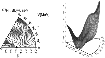
  Figure 2: Potential energy (relative to that of the spherical shape) for the ¹⁷⁸Hf nucleus calculated using the SLy4 Skyrme interaction plus the constant $G$ pairing.

  

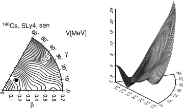
  Figure 3: Potential energy for the ¹⁹⁰Os nucleus, see also caption to figure 2.

  

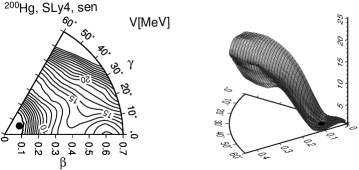
  Figure 4: Potential energy for the ²⁰⁰Hg nucleus, see also caption to figure 2.

  

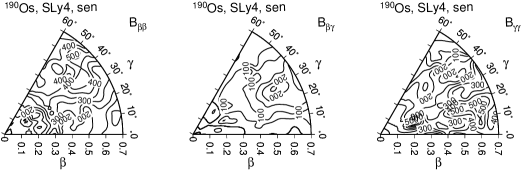
  Figure 5: Vibrational inertial functions $B_{\beta\beta}$, $B_{\beta\gamma}$, $B_{\gamma\gamma}$ (in $\hbar^{2}$/MeV) for the ¹⁹⁰Os nucleus.

  

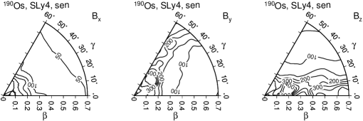
  Figure 6: Rotational inertial functions $B_{u}$, $u=x,y,z$ (in $\hbar^{2}$/MeV) for the ¹⁹⁰Os nucleus.

  

  Figure 7: Lowest collective energy levels for ¹⁷⁸Hf — ²⁰⁰Hg nuclei. Upper panels: $2_{1}$ and $4_{1}$ levels in the g.s. band. Lower panels: $2_{2}$ and $0_{2}$ levels. Experimental data taken from [118].

  

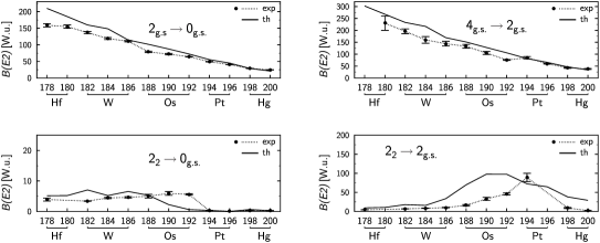
  Figure 8: Selected $B(E2)$ transition probabilities (in W.u.) in the ¹⁷⁸Hf — ²⁰⁰Hg nuclei. Upper panels: transitions within the ground state band, lower panels: $2_{2}\rightarrow 0_{\rm g.s.}$ and $2_{2}\rightarrow 2_{\rm g.s.}$. Note the different scales in various panels. Experimental data taken from [118].

  4.5 Extension of the collective space

  We end this section with a brief discussion of ideas concerning the extension of the collective space to variables connected with the pairing degrees of freedom. Some vague suggestions about such possibility can be found already in [6, 15]. In the simplest version of the collective approach to pairing, appropriate for the constant $G$ interaction, the pairing gap $\Delta$, which enters the formulae for the $v_{\mu}$, $u_{\mu}$ coefficients, is treated as a variable and not a solution of the BCS equations. In this way a family of states is parametrized by $\Delta$ and the ATDHFB [44] or the GCM+GOA [22, 92] methods allow to obtain the collective pairing Hamiltonian. The case of the state dependent pairing needs a slightly different definition of a collective variable instead of $\Delta$, see e.g. [119]. Usually one also considers a second variable, the gauge angle, which is used to implement the projection on a fixed number of particles. An important consequence of the collective treatment of the pairing is that one gets probability distributions in the $\Delta$ variable (coming from eigenfunctions of the collective pairing Hamiltonian) instead of a single value of the pairing gap. It is well known that values of the inertial functions entering the Bohr Hamiltonian strongly depend on the value of the pairing gap. Hence it is important to estimate the influence of the extension of the collective space on the spectrum and other properties of the Hamiltonian.

  If both quadrupole and pairing variables are combined, the resulting extended collective space is nine dimensional (four pairing variables for two kinds of nucleons). In principle one can use the methods from sections 4.1 or 4.2 to construct the collective Hamiltonian also in this case [119]. However, a full analysis of such Hamiltonian would be very difficult so that one must resort to some approximations [77, 119]. Firstly, the terms which explicitly couple quadrupole and pairing variables are neglected. Secondly, the ground state of the pairing part of the Hamiltonian is determined to get the probability distribution in the $\Delta$ variable (for both protons and neutrons). In [77, 100] the inertial functions of the Bohr Hamiltonian were calculated using the value of the pairing gap corresponding to the maximum of the distribution while in [119] the inertial functions obtained for various values of $\Delta$ were averaged with the weight given by this distribution. Results of the cited papers show that the collective treatment of pairing can bring significant changes in the energy spectrum, but more extensive studies (also on more consistent methods of determining the pairing strength) are still needed.

  5 Summary

  The Bohr collective model was originally invented to describe quadrupole oscillations of nuclear surface in the spherical nuclei. It has been subsequently developed and successfully applied to the description of the quadrupole collective excitations in various deformed nuclei. The Bohr Hamiltonian can be treated either at the phenomenological level or can be derived from a microscopic many-body theory. In the present review we have leaned towards the latter treatment of the Bohr model. Microscopic theories give, as a rule, quite complicated collective Hamiltonians which are determined by a number of functions of the dynamical variables rather than by a number of parameters as it used to be in the phenomenological approaches. Therefore, it is important to study the most general under some natural conditions, form of the Bohr Hamiltonian. The basic assumption of the Bohr collective model is that the dynamical variables form a real electric quadrupole tensor. The detailed analysis of the isotropic tensor fields, presented in this review, allows us to study the tensor structure of various ingredients of the general Bohr collective model. Its specific version is determined by several scalar functions. The collective Hamiltonian is defined by the six scalar inertial functions, the scalar weight and the (obviously scalar) potential — eight scalar functions of two scalar variables altogether. To define other collective observables we still need a number of additional scalar functions. The knowledge of the universal tensor structure of the collective wave functions allows us to express them also through scalar functions specific for a definite eigenstate of a given Hamiltonian.

  The scalar functions defining the model can be calculated in the framework of a microscopic theory. In practice it is the components of the inertial bitensor rather than the scalar inertial functions themselves that are calculated. There are the two fundamental methods to obtain the Bohr Hamiltonian from the many-body theory. One is the Adiabatic Time Dependent Hartree-Fock-Bogolyubov approach which, since it treats the collective motion as the classical motion of a wave packet, gives the classical and not the quantum Hamiltonian. Quantization of the classical Hamiltonian obtained in this method can lead to an ambiguity in the collective potential. The other method is provided by the Gaussian Overlap Approximation of the Generator Coordinate Method. It directly gives the quantum second order differential collective Hamiltonian (without the Gaussian Overlap Approximation the Generator Coordinate Methods leads to integral equations). Both methods mentioned above can be applied to different microscopic models. A whole range of the nuclear many-body theories are available: the phenomenological mean field models with different single-particle potentials such as the Nilsson or the Woods-Saxon ones, the self-consistent approaches with the Skyrme or the Gogny effective nucleon-nucleon forces and the Relativistic Mean Field theory. The presented example of application of the reviewed approach to the ¹⁷⁸Hf — ²⁰⁰Hg nuclei shows that the Bohr Hamiltonian derived from the effective interaction is a very useful tool for explaining nuclear collective properties. In addition, having the Bohr Hamiltonian obtained from the microscopic theory, one can try to examine another question which recently attracted attention, that is of the possible foundations of phenomenological models inspired partly by the Interacting Boson Model [67, 66]. This would require, however, a more extensive and detailed discussion which goes beyond the scope of the present review.

  Appendix A Spherical tensors and tensor fields

  In the nuclear collective models the operands are most often tensors under the O(3) group of orthogonal transformations in the three-dimensional physical space. The models employ tensor fields such as potentials, inertial functions, etc., which are usually isotropic functions of the dynamical variables. Here, in order to fix the notions and notation, we collect the definitions and properties of quantities and operations appearing in the theory of spherical tensors. We also briefly present the structure of the isotropic tensor fields, which is not so widely known.

  A.1 Spherical tensors

  A set of $2\lambda+1$ covariant components $\alpha_{\lambda\mu}$ with projections (magnetic numbers) $\mu=-\lambda,\,-\lambda+1,\,\dots\,,\lambda-1,\,\lambda$, representing an object (a c-number, an operator, etc.) $\alpha_{\lambda}$ in a three-dimensional coordinate system U, forms the SO(3) irreducible spherical tensor of rank $\lambda$ if

  $$\alpha^{\prime}_{\lambda\mu^{\prime}}=\sum_{\mu=-\lambda}^{\lambda}D^{\lambda\ast}_{\mu\mu^{\prime}}(\varphi,\vartheta,\psi)\alpha_{\lambda\mu}$$ (2.3eizabadahaoapgprsvwaeagahaiascaeamana)

  where $\alpha^{\prime}_{\lambda\mu^{\prime}}$ are the components representing the same object $\alpha_{\lambda}$ in the coordinate system U^′ rotated with respect to U by the Euler angles $\varphi$, $\vartheta$, $\psi$, and $D^{\lambda}_{\mu^{\prime}\mu}(\varphi,\vartheta,\psi)$ are the Wigner functions (rotation matrices) [34, 36]. The Wigner functions defined in [34] are complex conjugate of those of Bohr and Mottelson [36]. In nuclear physics the convention of Bohr and Mottelson is most widely used and we adopt it in this work. We do not quote here various useful properties of the Wigner functions as they can be found easily for instance in [34]. Only integer ranks $\lambda$ are considered here.

  In the special case of a rotation by the Euler angle $\varphi$ with $\vartheta=0$, $\psi=0$ (i.e. of a rotation about $z$-axis) formula (2.3eizabadahaoapgprsvwaeagahaiascaeamana) reduces to

  $$\alpha^{\prime}_{\lambda\mu^{\prime}}=\sum_{\mu}\rme^{-\rmi\mu\varphi}\delta_{\mu\mu^{\prime}}\alpha_{\lambda\mu}$$ (2.3eizabadahaoapgprsvwaeagahaiascaeamanb)

  A tensor whose only nonvanishing components is $\alpha_{\lambda 0}$ (i.e. $\alpha_{\lambda\mu}=0$ for $\mu\neq 0$) is invariant under such rotations, and can be called the axially symmetric tensor ($z$ is the symmetry axis). In general, a SO(3) tensor transforming under rotations as in (2.3eizabadahaoapgprsvwaeagahaiascaeamana), does not have a definite transformation rule under the inversion of the coordinate system, which supplements the rotations to the O(3) group. However, every SO(3) tensor can be decomposed into the two terms

  $$\alpha_{\lambda\mu}=\alpha_{\lambda\mu}^{(\mathrm{E})}+\alpha_{\lambda\mu}^{(\mathrm{M})}$$ (2.3eizabadahaoapgprsvwaeagahaiascaeamanc)

  called the proper (polar or electric) and the pseudo- (axial or magnetic) tensor, respectively, with the following transformation properties:

  $${\alpha_{\lambda\mu}^{(\mathrm{E})}}^{\prime\prime}=(-1)^{\lambda}\alpha_{\lambda\mu}^{(\mathrm{E})}$$ (2.3eizabadahaoapgprsvwaeagahaiascaeamand)

  and

  $${\alpha_{\lambda\mu}^{(\mathrm{M})}}^{\prime\prime}=(-1)^{\lambda+1}\alpha_{\lambda\mu}^{(\mathrm{M})}$$ (2.3eizabadahaoapgprsvwaeagahaiascaeamane)

  where the double prime denotes the components of the corresponding tensors in the coordinate system U^′′ whose axes are reflected with respect to those of U. The sign factors on the right-hand sides of (2.3eizabadahaoapgprsvwaeagahaiascaeamand) and (2.3eizabadahaoapgprsvwaeagahaiascaeamane) are the parities. Further below, the superscripts (E) or (M) will be omitted when the parity is not relevant. In general, the components $\alpha_{\lambda\mu}$ are complex numbers. However, in physical application most frequently real spherical tensors appear whose components are determined by $2\lambda+1$ real numbers up to a single phase factor. More precisely, the complex components of such tensors satisfy the following relations

  $$\alpha^{\ast}_{\lambda\mu}=\rme^{2\rmi\delta(\lambda)}(-1)^{-\mu}\alpha_{\lambda-\mu}.$$ (2.3eizabadahaoapgprsvwaeagahaiascaeamanf)

  Relations (2.3eizabadahaoapgprsvwaeagahaiascaeamanf) are preserved by the transformations (2.3eizabadahaoapgprsvwaeagahaiascaeamana). In the following the common phase is set to zero ($\delta(\lambda)=0$) as in the case of the standard spherical harmonics $Y_{\lambda\mu}$. Equation (2.3eizabadahaoapgprsvwaeagahaiascaeamanf) suggests that the tensor $\alpha_{\lambda}$ can be presented in the following form:

  $$\alpha_{\lambda 0}=a_{\lambda 0}\qquad\alpha_{\lambda\mu}=\frac{1}{\sqrt{2}}(a_{\lambda\mu}+ib_{\lambda\mu})\qquad\alpha_{\lambda-\mu}=\frac{(-1)^{\mu}}{\sqrt{2}}(a_{\lambda\mu}-ib_{\lambda\mu})$$ (2.3eizabadahaoapgprsvwaeagahaiascaeamang)

  for $\mu>0$. Thus, the tensor $\alpha_{\lambda}$ is indeed determined by the $2\lambda+1$ real numbers: the real and imaginary parts, $a_{\lambda\mu}\;(\mu=0,\,1,\,\dots,\lambda)$ and $b_{\lambda\mu}\;(\mu=1,\,\dots,\lambda)$, respectively, of the complex components $\alpha_{\lambda\mu}$ for $\mu\geq 0$.

  Coupling two real tensors, $\alpha_{\lambda}$ and $\chi_{\kappa}$, of ranks $\lambda$ and $\kappa$ and the zero phases in the following way

  $$[\alpha_{\lambda}\times\chi_{\kappa}]_{LM}=\sum_{\mu\nu}(\lambda\mu\kappa\nu|LM)\alpha_{\lambda\mu}\chi_{\kappa\nu},$$ (2.3eizabadahaoapgprsvwaeagahaiascaeamanh)

  where $(\lambda\mu\kappa\nu|LM)$ is the Clebsch-Gordan coefficient, one obtains a real tensor of rank $L$, where $|\lambda-\kappa|\leq L\leq\lambda+\kappa$, called an irreducible tensor product. Its phase is determined by the relation

  $$[\alpha_{\lambda}\times\chi_{\kappa}]_{LM}^{\ast}=(-1)^{L-M-\lambda-\kappa}[\alpha_{\lambda}\times\chi_{\kappa}]_{L-M}.$$ (2.3eizabadahaoapgprsvwaeagahaiascaeamani)

  The scalar product of the two real tensors of the same rank, $\alpha_{\lambda}$ and $\chi_{\lambda}$, is defined as

  $$(\alpha_{\lambda}\cdot\chi_{\lambda})=(-1)^{-\lambda}\sqrt{2\lambda+1}[\alpha_{\lambda}\times\chi_{\lambda}]_{00}.$$ (2.3eizabadahaoapgprsvwaeagahaiascaeamanj)

  It is also convenient to formally introduce the contravariant components $\alpha_{\lambda}^{\phantom{\lambda}\mu}$ of a tensor $\alpha_{\lambda}$ by relation

  $$\alpha_{\lambda}^{\phantom{\lambda}\mu}=\alpha_{\lambda\mu}^{\ast}.$$ (2.3eizabadahaoapgprsvwaeagahaiascaeamank)

  The scalar product can then be written as

  $$(\alpha_{\lambda}\cdot\chi_{\lambda})=\sum_{\mu}(-1)^{\mu}\alpha_{\lambda\mu}\chi_{\lambda-\mu}=\sum_{\mu}\alpha_{\lambda\mu}\chi_{\lambda\mu}^{\ast}=\sum_{\mu}\alpha_{\lambda\mu}\chi_{\lambda}^{\phantom{\lambda}\mu}.$$ (2.3eizabadahaoapgprsvwaeagahaiascaeamanl)

  The square of a tensor $\alpha_{\lambda}$ expressed in terms of the variables $a_{\lambda\mu}$ and $b_{\lambda\mu}$ reads

  $$(\alpha_{\lambda}\cdot\alpha_{\lambda})=\sum_{\mu=0}^{\lambda}a^{2}_{\lambda\mu}+\sum_{\mu=1}^{\lambda}b^{2}_{\lambda\mu}.$$ (2.3eizabadahaoapgprsvwaeagahaiascaeamanm)

  This shows that $a_{\lambda}$’s and $b_{\lambda}$’s can play the role of the Cartesian coordinates in the $(2\lambda+1)$-dimensional Euclidean space, whose volume element is

  $$\mathrm{d}\Omega=\prod_{\mu=0}^{\lambda}\mathrm{d}a_{\lambda\mu}\prod_{\mu=1}^{\lambda}\mathrm{d}b_{\lambda\mu}.$$ (2.3eizabadahaoapgprsvwaeagahaiascaeamann)

  Let this Euclidean space be infinite, i.e. $-\infty<a_{\lambda\mu},b_{\lambda\mu}<\infty$ for all $\mu$’s. The scalar product in the Hilbert space H_Ω of functions of the Cartesian coordinates $a_{\lambda\mu},\ b_{\lambda\mu}$ is defined in the usual way by

  $$\langle\Psi|\Phi\rangle=\int\Psi^{\ast}(a_{\lambda},b_{\lambda})\Phi(a_{\lambda},b_{\lambda})\rmd\Omega.$$ (2.3eizabadahaoapgprsvwaeagahaiascaeamano)

  The integral is over the whole space.

  Apart from the spherical tensors, the bitensors or matrices with tensor indices also appear in the collective models. The spherical bitensor is defined in a similar way as the tensor, namely

  $$M^{\prime}_{\lambda\mu^{\prime},\kappa\nu^{\prime}}=\sum_{\mu\nu}D^{\lambda\ast}_{\mu\mu^{\prime}}(\varphi,\vartheta,\psi)D^{\kappa\ast}_{\nu\nu^{\prime}}(\varphi,\vartheta,\psi)M_{\lambda\mu,\kappa\nu}$$ (2.3eizabadahaoapgprsvwaeagahaiascaeamanp)

  where $M_{\lambda\mu,\kappa\nu}$ and $M^{\prime}_{\lambda\mu^{\prime},\kappa\nu^{\prime}}$ are the components of the bitensor $M_{\lambda,\kappa}$ in the coordinate systems U and U^′, respectively. The bitensor $M_{\lambda,\kappa}$ can always be decomposed into a number of tensors $T^{(\lambda\kappa)}_{LM}$ of ranks $L$, where $|\lambda-\kappa|\leq L\leq\lambda+\kappa$, as follows:

  $$M_{\lambda\mu,\kappa\nu}=\sum_{LM}(\lambda\mu\kappa\nu|LM)T^{(\lambda\kappa)}_{LM}.$$ (2.3eizabadahaoapgprsvwaeagahaiascaeamanq)

  If a matrix of the bitensor $M_{\lambda,\lambda}$ is symmetric the summation in (2.3eizabadahaoapgprsvwaeagahaiascaeamanq) is restricted to even $L$’s. The scalar product of a bitensor $M_{\lambda,\kappa}$ and a tensor $\alpha_{\kappa}$ is defined similarly to (2.3eizabadahaoapgprsvwaeagahaiascaeamanl)

  $$(M_{\lambda\mu,\kappa}\cdot\alpha_{\kappa}) = \sum_{\nu}(-1)^{\nu}M_{\lambda\mu,\kappa-\nu}\alpha_{\kappa\nu}=\sum_{\nu}M_{\lambda\mu,\kappa}^{\phantom{\lambda\mu\kappa}\nu}\alpha_{\kappa\nu}$$ (2.3eizabadahaoapgprsvwaeagahaiascaeamanr)

  $$(\alpha_{\lambda}\cdot M_{\lambda,\kappa\nu}) = \sum_{\mu}(-1)^{\mu}\alpha_{\lambda\mu}M_{\lambda-\mu,\kappa\nu}=\sum_{\mu}\alpha_{\lambda\mu}M_{\lambda\phantom{\mu},\kappa\nu}^{\phantom{\lambda}\mu}.$$ (2.3eizabadahaoapgprsvwaeagahaiascaeamans)

  The differential operators

  $$\hat{p}_{\lambda\mu}=-\rmi\hbar\frac{\partial}{\partial a_{\lambda\mu}}\qquad\hat{q}_{\lambda\mu}=-\rmi\hbar\frac{\partial}{\partial b_{\lambda\mu}}$$ (2.3eizabadahaoapgprsvwaeagahaiascaeamant)

  are Hermitian in H_Ω and play the role of the momenta canonically conjugate to the coordinates since they fulfill the following commutation relations

  $$[a_{\lambda\mu},\hat{p}_{\lambda\nu}]=\rmi\hbar\delta_{\mu\nu}\qquad[b_{\lambda\mu},\hat{p}_{\lambda\nu}]=0\qquad[a_{\lambda\mu},\hat{q}_{\lambda\nu}]=0\qquad[b_{\lambda\mu},\hat{q}_{\lambda\nu}]=\rmi\hbar\delta_{\mu\nu}.$$ (2.3eizabadahaoapgprsvwaeagahaiascaeamanu)

  The covariant tensor operator of momentum is defined as

  $$\hat{\pi}_{\lambda\mu}=\frac{1}{\sqrt{2}}(\hat{p}_{\lambda\mu}+\rmi\hat{q}_{\lambda\mu})=-\rmi\hbar\frac{\partial}{\partial\alpha^{\ast}_{\lambda\mu}}=-\rmi\hbar\frac{\partial}{\partial\alpha_{\lambda}^{\phantom{\lambda}\mu}}.$$ (2.3eizabadahaoapgprsvwaeagahaiascaeamanv)

  The relations inverse to (2.3eizabadahaoapgprsvwaeagahaiascaeamang) have been used here to express the derivatives with respect to $\alpha_{\lambda\mu}$ through the derivatives with respect to $a_{\lambda\mu}$ and $b_{\lambda\mu}$. The momentum tensor Hermitian adjoint to $\hat{\pi}_{\lambda\mu}$ is

  $$\hat{\pi}_{\lambda\mu}^{{\dagger}}=\frac{1}{\sqrt{2}}(\hat{p}_{\lambda\mu}-\rmi\hat{q}_{\lambda\mu})=-\rmi\hbar\frac{\partial}{\partial\alpha_{\lambda\mu}}.$$ (2.3eizabadahaoapgprsvwaeagahaiascaeamanw)

  It plays the role of the momentum tensor canonically conjugate to the coordinate tensor $\alpha_{\lambda}$ since it fulfills the following commutation relation:

  $$[\alpha_{\lambda\mu},\hat{\pi}_{\lambda\nu}^{{\dagger}}]=\rmi\hbar\delta_{\mu\nu}.$$ (2.3eizabadahaoapgprsvwaeagahaiascaeamanx)

  It follows from (2.3eizabadahaoapgprsvwaeagahaiascaeamana) that the Hermitian adjoint momentum operator (2.3eizabadahaoapgprsvwaeagahaiascaeamanw) has the transformation properties of the contravariant and not the covariant tensor in spite of the convention of notation of (2.3eizabadahaoapgprsvwaeagahaiascaeamank). According to the convention (2.3eizabadahaoapgprsvwaeagahaiascaeamank)

  $$\hat{\pi}_{\lambda}^{\phantom{\lambda}\mu}=\rmi\hbar\frac{\partial}{\partial\alpha_{\lambda\mu}}=-\hat{\pi}_{\lambda\mu}^{{\dagger}}.$$ (2.3eizabadahaoapgprsvwaeagahaiascaeamany)

  Obviously, the momentum tensor is of the same parity as the conjugate coordinate tensor. It is easy to check that the differential operator

  $$\hat{L}_{1\mu}^{(\lambda)}=\rmi(-1)^{\lambda}\sqrt{\frac{\lambda(\lambda+1)(2\lambda+1)}{3}}[\alpha_{\lambda}\times\hat{\pi}_{\lambda}]_{1\mu}$$ (2.3eizabadahaoapgprsvwaeagahaiascaeamanz)

  obeys the following commutation relations:

  $$[\hat{L}_{1\nu}^{(\lambda)},\alpha_{\lambda\mu}]=\sqrt{\lambda(\lambda+1)}(\lambda\mu 1\nu|\lambda\mu+\nu)\alpha_{\lambda\mu+\nu}$$ (2.3eizabadahaoapgprsvwaeagahaiascaeamanaa)

  and

  $$[\hat{L}_{1\nu}^{(\lambda)},\hat{\pi}_{\lambda\mu}]=\sqrt{\lambda(\lambda+1)}(\lambda\mu 1\nu|\lambda\mu+\nu)\hat{\pi}_{\lambda\mu+\nu}\ .$$ (2.3eizabadahaoapgprsvwaeagahaiascaeamanab)

  This means that $\hat{L}_{1\mu}^{(\lambda)}$ is the angular momentum operator acting in the space of functions of $\alpha_{\lambda\mu}$ (cf [34]). The angular momentum (2.3eizabadahaoapgprsvwaeagahaiascaeamanz) is always an axial vector irrespective of the parity of $\alpha_{\lambda}$ and $\hat{\pi}_{\lambda}$. Equations (2.3eizabadahaoapgprsvwaeagahaiascaeamanz), (2.3eizabadahaoapgprsvwaeagahaiascaeamanaa) and (2.3eizabadahaoapgprsvwaeagahaiascaeamanab) lead to the obvious commutation relations for the components of the angular momentum

  $$[\hat{L}_{1\mu}^{(\lambda)},\hat{L}_{1\nu}^{(\lambda)}]=-\hbar\sqrt{2}(1\mu 1\nu|1\kappa)\hat{L}_{1\kappa}^{(\lambda)}.$$ (2.3eizabadahaoapgprsvwaeagahaiascaeamanac)

  A.2 Isotropic tensor fields

  In continuum mechanics there appears the notion of an isotropic function of variables which are the components of a tensor (cf [120]). Roughly speaking, the function is isotropic if no parameters with tensor properties (e.g. material tensors) enter its definition. The isotropic functions which are tensors themselves, are called the isotropic tensor fields. The isotropic tensor field $T_{LM}(\alpha_{\lambda})$ of rank $L$ obeys the following transformation rule:

  $$T^{\prime}_{LM^{\prime}}(\alpha_{\lambda\mu})=T_{LM^{\prime}}(\alpha_{\lambda\mu}^{\prime})=\sum_{M=-L}^{L}D^{L\ast}_{MM^{\prime}}(\varphi,\vartheta,\psi)T_{LM}(\alpha_{\lambda\mu})$$ (2.3eizabadahaoapgprsvwaeagahaiascaeamanad)

  where $T_{LM}$ and $\alpha_{\lambda\mu}$ are the components of tensors $T_{L}$ and $\alpha_{\lambda}$ in the original system U whereas $T^{\prime}_{LM^{\prime}}$ and $\alpha^{\prime}_{\lambda\mu}$ are the respective components in the rotated system U^′. Equation (2.3eizabadahaoapgprsvwaeagahaiascaeamanad) states that to transform the field $T_{LM}(\alpha_{\lambda})$ it is sufficient to transform its tensor argument $\alpha_{\lambda\mu}$. It would not be so for a tensor field which is not isotropic.

  The question arises to what extent the form of functional dependence of the isotropic tensor field $T_{LM}(\alpha_{\lambda})$ on the tensor $\alpha_{\lambda}$ is determined solely by their tensor properties. To answer this question we present below a scheme of constructing an arbitrary spherical tensor as a function of another spherical tensor. It turns out that for a given rank $\lambda$ there exists a finite complete system of $i_{\lambda}$ irreducible (i.e. none of them can be expressed rationally and integrally in terms of the others) elementary tensors $\varepsilon_{ilm}(\alpha_{\lambda})$, $i=1,...,i_{\lambda}$, of different ranks $l$. The highest components $(m=l)$ of the elementary tensors are called the elementary factors [40]. The elementary tensors are constructed by coupling successively $n$ tensors $\alpha_{\lambda}$ to different $l$’s, $l<n\lambda$:

  $$\varepsilon_{ilm}(\alpha_{\lambda})\equiv\varepsilon_{lm}^{(n)}(\alpha_{\lambda}[\mathrm{c}])=[\underbrace{\alpha_{\lambda}\times\dots\times\alpha_{\lambda}}_{n}]_{lm}^{[\mathrm{c}]},$$ (2.3eizabadahaoapgprsvwaeagahaiascaeamanae)

  where the symbol [c], redundant in most cases, specifies the coupling scheme. Tensor $\alpha_{\lambda}=\varepsilon_{\lambda}^{(1)}$ itself is an elementary tensor. The scalar product of two tensors $\alpha_{\lambda}$, $(\alpha_{\lambda}\cdot\alpha_{\lambda})=\varepsilon_{0}^{(2)}$ as well as all other independent scalars are the elementary factors. Completeness of the system of elementary factors does not mean that relations between them must not exist. On the contrary, some relations between them, called syzygies, do exist. They take the form:

  $$S_{j}(\varepsilon_{1ll},\dots,\varepsilon_{i_{\lambda}l^{\prime}l^{\prime}})=0$$ (2.3eizabadahaoapgprsvwaeagahaiascaeamanaf)

  with $j=1,\dots,j_{\lambda}$, where $S_{j}$ are some rational integral functions. The number of independent syzygies is finite and depends on the rank $\lambda$. It turns out that to obtain a tensor of a given rank $L$, it is sufficient to align (i.e. to couple to the maximal angular momentum) the elementary tensors. The alignment of the elementary tensors means the multiplication of the elementary factors (the relevant Clebsch-Gordan coefficients are all equal to 1). Because of the existence of the syzygies (2.3eizabadahaoapgprsvwaeagahaiascaeamanaf), some of the aligned tensors

  $$[\varepsilon_{l}^{(n)}(\alpha_{\lambda}[\mathrm{c}])\times\varepsilon_{l^{\prime}}^{(n^{\prime})}(\alpha_{\lambda}[\mathrm{c^{\prime}}])\times\dots]_{L=l+l^{\prime}+\dots}$$

  can be expressed rationally and integrally in terms of the others. Using the syzygies the finite number $k_{\lambda L}$ of independent aligned tensors $\tau_{kLM}(\varepsilon)$ with $k=1,\dots,k_{\lambda L}$ can be found. These independent aligned tensors are called fundamental tensors. This is because an arbitrary tensor field of rank $L$, being the isotropic function of tensor $\alpha_{\lambda}$, can always be written in the form:

  $$T_{LM}(\alpha_{\lambda}) = \sum_{k=1}^{k_{\lambda L}}f_{k}(\varepsilon_{0})\tau_{kLM}(\varepsilon)$$ (2.3eizabadahaoapgprsvwaeagahaiascaeamanag)

  where argument $\varepsilon_{0}$ of $f_{k}$ stands for all independent scalars. Scalar functions $f_{k}$ can be, in general, arbitrary. However, the form of some of $f_{k}$ can be restricted. For instance, some scalar $\varepsilon_{0}$ cannot appear in it in too high power. This is because a syzygy can make the expression $(\varepsilon_{i00})^{n}(\varepsilon_{i^{\prime}ll})^{n^{\prime}}$ for some $i$, $i^{\prime}$, $n$ and $n^{\prime}$ dependent on other elementary factors. When $\alpha_{\lambda}$ has the positive parity, an arbitrary field of the form (2.3eizabadahaoapgprsvwaeagahaiascaeamanag) has obviously the positive parity as well. However, when $\alpha_{\lambda}$ has the negative parity, the field $T_{L}$ has, in general, no definite parity. To decompose it into the parts of the positive and the negative parity, the parities of the scalars and the fundamental tensors should be taken into account. This can easily be done by noticing that the parity of an elementary tensor $\varepsilon_{l}^{(n)}([\mathrm{c}])$ is $(-1)^{n}$.

  A justification of the procedure presented above can be traced back to the theory of covariants of algebraic forms given by Dickson [121], which, however, uses different notions than these used in the present paper. Let us sketch the main points of this theory (cf [122, 37]). Let the binary (in variables $x_{1},\,x_{2}$) $2\lambda$-ic (of order $2\lambda$) algebraic form be

  $$F_{2\lambda}(x_{1},x_{2};\alpha_{\lambda-\lambda},\dots,\alpha_{\lambda\lambda})=\sum_{\mu=-\lambda}^{\lambda}\left(\begin{array}[]{c}2\lambda\\ \lambda-\mu\end{array}\right)^{1/2}\alpha_{\lambda\mu}x_{1}^{\lambda+\mu}x_{2}^{\lambda-\mu}$$ (2.3eizabadahaoapgprsvwaeagahaiascaeamanaj)

  with a set of coefficients $(\alpha_{\lambda\mu}$, $\mu=-\lambda,\dots,\lambda)$. Changing in (2.3eizabadahaoapgprsvwaeagahaiascaeamanaj) the variables by a linear non-singular transformation

  $$x_{i}=\sum_{k=1}^{2}A_{ik}y_{k}$$ (2.3eizabadahaoapgprsvwaeagahaiascaeamanak)

  where $i=1,2$, one obtains

  $$F_{2\lambda}(x_{1},x_{2};\alpha_{\lambda})=G_{2\lambda}(y_{1},y_{2};\alpha_{\lambda})=\sum_{\mu=-\lambda}^{\lambda}\left(\begin{array}[]{c}2\lambda\\ \lambda-\mu\end{array}\right)^{1/2}\chi_{\lambda\mu}(\alpha_{\lambda})y_{1}^{\lambda+\mu}y_{2}^{\lambda-\mu}$$ (2.3eizabadahaoapgprsvwaeagahaiascaeamanan)

  with a new set of coefficients $(\chi_{\lambda\mu},\,\mu=-\lambda,\dots,\lambda)$. The $2l$-ic form

  $$H_{2l}^{(n)}(x_{1},x_{2};\alpha_{\lambda}) = \sum_{m=-l}^{l}\left(\begin{array}[]{c}2l\\ l-m\end{array}\right)^{1/2}h_{lm}^{(n)}(\alpha_{\lambda})x_{1}^{l+m}x_{2}^{l-m},$$ (2.3eizabadahaoapgprsvwaeagahaiascaeamanaq)

  such that

  $$H_{2l}^{(n)}(y_{1},y_{2};\chi_{\lambda})=(\mathrm{det}(A_{ik}))^{w}H_{2l}^{(n)}(x_{1},x_{2};\alpha_{\lambda})$$ (2.3eizabadahaoapgprsvwaeagahaiascaeamanas)

  is called a (homogeneous) covariant with the weight $w$ of $F_{2\lambda}$. Coefficients $h_{lm}^{(n)}$ are homogeneous polynomials of order $n$ (called the degree of the covariant) such that $\lambda n=l+w$. For $l=0$ the form $H_{0}^{(n)}=h_{00}^{(n)}$ is called an invariant of $F_{2\lambda}$. The polynomial in front of the highest power of $x_{1}$ in (2.3eizabadahaoapgprsvwaeagahaiascaeamanaq), $h_{ll}^{(n)}$, is called a semi-invariant of $F_{2\lambda}$. It can be shown in the theory of covariants of algebraic forms that any covariant can be expressed rationally and integrally in terms of a finite, irreducibly complete set of covariants, which can be related rationally and integrally to each other by a finite system of independent syzygies (Gordan-Hilbert Finiteness Theorem, see [122]). The number of the basis covariants for a few lowest $\lambda$’s is listed in [37].

  It remains to answer the question of what the covariants of algebraic forms have in common with the tensor fields being functions of tensors. It turns out that the semi-invariant $h_{ll}^{(n)}(\alpha_{\lambda})$ forms the component of the highest projection of a tensor field of rank $l$ depending on the tensor of rank $\lambda$ (the highest weight of an irreducible representation of SO(3) embedded in an irreducible representation of SU($2\lambda+1$)). The other polynomials $h_{lm}^{(n)}(\alpha_{\lambda})$ in (2.3eizabadahaoapgprsvwaeagahaiascaeamanaq) are the remaining components of the same tensor. A proof of this statement is demonstrated briefly in reference [123]. Constructive proofs of the form (2.3eizabadahaoapgprsvwaeagahaiascaeamanag) can be carried through by explicitly constructing a basis in the space of functions of $\alpha_{\lambda}$ and showing that it has the structure as in (2.3eizabadahaoapgprsvwaeagahaiascaeamanag). In the case of $\lambda=1$ it is well known from textbooks of quantum mechanics that an arbitrary tensor field of rank $L$ which is a function of the position vector $\bi{r}$ takes the form:

  $$T_{LM}(\bi{r})=f_{L}(r)Y_{LM}(\frac{\bi{r}}{r})$$ (2.3eizabadahaoapgprsvwaeagahaiascaeamanat)

  where $r^{2}=\bi{r}{\cdot}\bi{r}$ and $Y_{LM}$ is the corresponding spherical harmonic. From (2.3eizabadahaoapgprsvwaeagahaiascaeamanat) it is seen immediately that in the case of $\lambda=1$ there are the two elementary tensors $(i_{1}=2)$, namely the vector $\bi{r}$ and the scalar $r^{2}$, and no syzygy $(j_{1}=0)$. Moreover, for every given $L$ there is only one fundamental tensor $(k_{1L}=1)$ of the form [34]:

  $$\tau_{LM}(\bi{r})=[\underbrace{\bi{r}\times\bi{r}\times\dots\times\bi{r}}_{L}]_{LM}\propto r^{L}Y_{LM}(\frac{\bi{r}}{r}).$$ (2.3eizabadahaoapgprsvwaeagahaiascaeamanau)

  Constructions of the oscillator bases in the cases of $\lambda=2$ (see [42] and references quoted therein) and $\lambda=3$ [123] have been also performed confirming the form (2.3eizabadahaoapgprsvwaeagahaiascaeamanag).

  Appendix B Properties of the ATDHFB inertial functions in the intrinsic frame

  B.1 (In)dependence on the Euler angles.

  In this Appendix the three Euler angles $(\varphi,\vartheta,\psi)$ will be compactly denoted as $\boldsymbol{\varphi}$ or $\varphi_{j}$, $j{=}1,2,3$. The BCS-type states depending on the deformation and the Euler angles $\boldsymbol{\varphi}$ are constructed as $U(\boldsymbol{\varphi})|\Phi(\boldsymbol{q})\rangle$ where $|\Phi(\boldsymbol{q})\rangle$ is the BCS state in the intrinsic frame and $\boldsymbol{q}$ stands for any of the pairs of the deformation variables: $(a_{0},a_{2})$, $(q_{0},q_{2})$ or $(\beta,\gamma)$. $U(\boldsymbol{\varphi})$ is the rotation operator in the Fock space. The argument $\boldsymbol{\varphi}$ will sometimes be dropped for the sake of brevity. The density matrix ${\cal R}_{0}(\boldsymbol{q},\boldsymbol{\varphi})$ can be written as

  $${\cal R}_{0}(\boldsymbol{q},\boldsymbol{\varphi})={\cal U}{\cal R}_{0}(\boldsymbol{q}){\cal U}^{+}$$ (2.3eizabadahaoapgprsvwaeagahaiascaeamana)

  where

  $${\cal U}=\left(\begin{array}[]{cc}u&0\\ 0&u^{*}\end{array}\right)\ .$$ (2.3eizabadahaoapgprsvwaeagahaiascaeamanb)

  $u$ is a matrix of $U(\boldsymbol{\varphi})$ in a fixed basis of the one-particle space. It fulfills the relation

  $$U^{+}d^{+}_{\mu}U=\sum_{\nu}u^{*}_{\mu\nu}d^{+}_{\nu}\ .$$ (2.3eizabadahaoapgprsvwaeagahaiascaeamanc)

  Equation (2.3eizabadahaoapgprsvwaeagahaiascaeamana) can be derived as follows (the $(11)$ block of the ${\cal R}_{0}$ is taken as an example):

  $$({\cal R}^{11}_{0}(q,\boldsymbol{\varphi}))_{mn}=\langle U\Phi(\boldsymbol{q})|d^{+}_{n}d_{m}\,|U\Phi(\boldsymbol{q})\rangle=\langle\Phi(\boldsymbol{q})|U^{+}d^{+}_{n}UU^{+}d_{m}\,U|\Phi(\boldsymbol{q})\rangle=$$

  $$=\sum_{jk}u^{*}_{nj}u_{mk}\langle\Phi(\boldsymbol{q})|d^{+}_{j}d_{k}\,|\Phi(\boldsymbol{q})\rangle=(u{\cal R}^{11}_{0}(\boldsymbol{q})u^{+})_{mn}\ .$$ (2.3eizabadahaoapgprsvwaeagahaiascaeamand)

  Now we show that the ATDHFB inertial functions do not depend on the Euler angles. To calculate the vibrational functions $B_{q_{i}q_{k}}$ one needs the derivatives of ${\cal R}_{0}(\boldsymbol{q},\boldsymbol{\varphi})$ with respect to the deformation variables. It is easy to show that the derivatives can be written analogously to (2.3eizabadahaoapgprsvwaeagahaiascaeamana), i.e. $\partial_{q_{j}}{\cal R}_{0}(\boldsymbol{q},\boldsymbol{\varphi})={\cal U}\partial_{q_{j}}{\cal R}_{0}(\boldsymbol{q}){\cal U}^{+}$. The same is true for ${\cal R}^{k}_{1}(\boldsymbol{q},\boldsymbol{\varphi})$ in view of (2.3eizabadahaoapgprsvwaeagahaiasch) and the properties of the induced self-consistent Hamiltonian ${\cal W}$. Consequently, all vibrational functions (which are proportional to the trace $\Tr_{2d}(R^{k}_{1}[\partial_{q_{j}}{\cal R}_{0},{\cal R}_{0}]$)) do not depend on the Euler angles.

  The rotational functions deserve a detailed treatment. Derivatives of ${\cal R}(\boldsymbol{q},\boldsymbol{\varphi})$ with respect to the Euler angles $\varphi_{j}$ are equal

  $$\partial_{\varphi_{j}}{\cal R}^{11}_{mn}(\boldsymbol{q},\boldsymbol{\varphi})=\langle\partial_{\varphi_{j}}U\Phi(\boldsymbol{q})|d^{+}_{n}d_{m}|U\Phi(\boldsymbol{q})\rangle+\langle U\Phi(\boldsymbol{q})|d^{+}_{n}d_{m}|\partial_{\varphi_{j}}U\Phi(\boldsymbol{q})\rangle=$$ (2.3eizabadahaoapgprsvwaeagahaiascaeamane)

  $$=\langle U^{-1}\partial_{\varphi_{j}}U\Phi(\boldsymbol{q})|U^{+}d^{+}_{n}d_{m}U|\Phi(\boldsymbol{q})\rangle+\langle\Phi(\boldsymbol{q})|U^{+}d^{+}_{n}d_{m}U|U^{-1}\partial_{\varphi_{j}}U\Phi(\boldsymbol{q})\rangle=$$ (2.3eizabadahaoapgprsvwaeagahaiascaeamanf)

  $$=(u\tilde{{\cal R}}^{11}_{0,j}(\boldsymbol{q},\boldsymbol{\varphi})u^{+})_{mn}$$ (2.3eizabadahaoapgprsvwaeagahaiascaeamang)

  where

  $$(\tilde{{\cal R}}^{11}_{0,j})_{mn}(\boldsymbol{q},\boldsymbol{\varphi})=\langle\Phi(\boldsymbol{q})|d^{+}_{n}d_{m}|U^{-1}\partial_{\varphi_{j}}U\Phi(\boldsymbol{q})\rangle+{\rm h.c.}$$ (2.3eizabadahaoapgprsvwaeagahaiascaeamanh)

  The operator $U^{-1}\partial_{\varphi_{j}}U$ can be expressed in terms of the generators of the rotation group

  $$U^{-1}\partial_{\varphi_{j}}U=\sum_{k}P_{kj}(\boldsymbol{\varphi})Y_{k}$$ (2.3eizabadahaoapgprsvwaeagahaiascaeamani)

  where $P(\boldsymbol{\varphi})$ is the universal (i.e. the same for all representations of the rotation group) matrix

  $$P=\left(\begin{array}[]{ccc}-\sin\vartheta\cos\psi,&\sin\psi,&0\\ \sin\vartheta\sin\psi,&\cos\psi,&0\\ \cos\vartheta,&0,&1\end{array}\right)$$ (2.3eizabadahaoapgprsvwaeagahaiascaeamanj)

  and $Y_{k}=-iJ_{k}/\hbar$, where $J_{k}$ are components of the angular momentum operator in the Fock space. Finally

  $$\tilde{{\cal R}}^{11}_{0,j}(\boldsymbol{q},\boldsymbol{\varphi})=\sum_{k}P_{kj}(\boldsymbol{\varphi})u{{\cal F}}^{11}_{k}(\boldsymbol{q})u^{+}$$ (2.3eizabadahaoapgprsvwaeagahaiascaeamank)

  where the matrices

  $$({\cal F}_{k}^{11}(\boldsymbol{q}))_{mn}=-\rmi\hbar^{-1}\langle\Phi(\boldsymbol{q})|d^{+}_{n}d_{m}J_{k}|\Phi(\boldsymbol{q})\rangle+{\rm h.c.}$$ (2.3eizabadahaoapgprsvwaeagahaiascaeamanl)

  do not depend on the Euler angles. Of course, all the blocks of the $\tilde{{\cal R}}_{0,j}(\boldsymbol{q},\boldsymbol{\varphi})$ matrix exhibit the same dependence on the Euler angles. Moreover, the matrices ${\cal R}_{1}$ behave in an analogous way, that is

  $${\cal R}_{1}^{l}=\dot{\varphi_{l}}\sum_{r}P_{rl}(\boldsymbol{\varphi}){{\cal U}}{{\cal Z}}_{r}(\boldsymbol{q}){{\cal U}}^{+}$$ (2.3eizabadahaoapgprsvwaeagahaiascaeamanm)

  where ${\cal Z}_{r}(\boldsymbol{q})$ do not depend on the Euler angles.

  Taking into account that the angular velocity in the body fixed frame is given by

  $$\omega_{j}=\sum_{k}P_{jk}\dot{\varphi_{k}}$$ (2.3eizabadahaoapgprsvwaeagahaiascaeamann)

  the rotational classical Hamiltonian can be written as

  $$H_{\rm cl,rot}=\frac{1}{2}\sum_{kj}I_{kj}\omega_{k}\omega_{j}$$ (2.3eizabadahaoapgprsvwaeagahaiascaeamano)

  with

  $$I_{kj}=\frac{\rmi\hbar}{2}\Tr_{2d}({\cal Z}_{k}[{\cal F}_{j},{\cal R}_{0}])$$ (2.3eizabadahaoapgprsvwaeagahaiascaeamanp)

  which obviously do not depend on the Euler angles.

  B.2 Block structure of the inertia tensor in the intrinsic frame

  Taking into account the ${\rm D}_{2}$ symmetry of the $|\Phi(\boldsymbol{q})\rangle$ state, one can prove the ATDHFB inertial functions give the classical kinetic energy which has the form identical with that of (2.3eizabadahaoapd)

  $$H_{\rm cl,kin}=H_{\rm cl,kin,vib}+H_{\rm cl,rot}$$ (2.3eizabadahaoapgprsvwaeagahaiascaeamanq)

  or, more precisely, that the vibration-rotational terms are absent and, moreover, that

  $$I_{kj}=\delta_{kj}I_{k}\ .$$ (2.3eizabadahaoapgprsvwaeagahaiascaeamanr)

  The sketch of the proof is as follows. The operators $S_{k}=\exp(-\rmi\pi J_{k}/\hbar)$ are the generators of the group ${\rm D}_{2}$ and invariance of the $|\Phi(\boldsymbol{q})\rangle$ with respect to the ${\rm D}_{2}$ group means that $S_{k}|\Phi(\boldsymbol{q})\rangle=|\Phi(\boldsymbol{q})\rangle$, which in the density matrix language can be rewritten as ${\cal S}_{k}{\cal R}_{0}{\cal S}^{+}_{k}={\cal R}_{0}$. The connection between $S_{k}$ and ${\cal S}_{k}$ is analogous to that between $U$ and ${\cal U}$ (cf (2.3eizabadahaoapgprsvwaeagahaiascaeamana) to (2.3eizabadahaoapgprsvwaeagahaiascaeamanc)). For the angular momentum in the Fock space one has $S^{+}_{k}J_{j}S_{k}=J_{j}$ for $k=j$ and $S^{+}_{k}J_{j}S_{k}=-J_{j}$ otherwise. In consequence, the matrices ${\cal F}_{j}$ and ${\cal Z}_{l}$ have the same property, i.e. ${\cal S}_{k}{\cal F}_{j}{\cal S}^{+}_{k}=\pm{\cal F}_{j}$. The formula (2.3eizabadahaoapgprsvwaeagahaiascaeamanr) follows from the definition (2.3eizabadahaoapgprsvwaeagahaiascaeamanp) of $I_{kj}$ and the properties of the trace. In a similar way one can verify that the mixed vibration-rotational parameters $B_{q_{i}\varphi_{j}}$ vanish.

  If $H_{\rm cl,rot}$ (2.3eizabadahaoapgprsvwaeagahaiascaeamano) is treated as an expression for the metric tensor in the space of rotation matrices and (2.3eizabadahaoapgprsvwaeagahaiascaeamanr) is valid, the corresponding Laplace-Beltrami operator has the form

  $$\sum_{k}\frac{1}{I_{k}}\tilde{L}^{2}_{k}$$ (2.3eizabadahaoapgprsvwaeagahaiascaeamans)

  where $\tilde{L}_{k}$ are the generators of the right regular representation of the SO(3) group. They are proportional to the collective angular momentum operators in the intrinsic frame, cf (2.3eio).

  References

References

- [1] Rayleigh Lord 1879 Proc. R. Soc. 29 71
- [2] von Weizsäcker C F 1935 Z. Phys. 96 431
- [3] Flügge S 1941 Ann. Phys., Lpz. 39 373
- [4] Bohr A 1952 K. Danske Vidensk. Selsk., Mat.-Fys. Medd. 26 no 14
- [5] Bohr A and Mottelson B R 1953 K. Danske Vidensk. Selsk., Mat.-Fys. Medd. 27 no 16
- [6] Belyaev S T 1965 Nucl. Phys. 64 17
- [7] Kumar K and Baranger M 1967 Nucl. Phys. A 92 608
- [8] Bohr A and Mottelson B R 1975 Nuclear Structure vol 2 (Reading: Benjamin) appendix 6B
- [9] Wilets L and Jean M 1956 Phys. Rev. 102 788
- [10] Davydov A S and Filippov G F 1958 Nucl. Phys. 8 237
- [11] Davydov A S and Chaban A A 1960 Nucl. Phys. 20 499
- [12] Faessler A and Greiner W 1962 Z. Phys. 168 425
- [13] Faessler A and Greiner W 1962 Z. Phys. 170 105
- [14] Faessler A, Greiner W and Sheline R K 1965 Nucl. Phys. 80 417
- [15] Baranger M and Kumar K 1968 Nucl. Phys. A 122 241
- [16] Baranger M and Vénéroni M 1978 Ann. Phys., NY 114 123
- [17] Baranger M 1961 Phys. Rev. 122 992
- [18] Sawicki J 1961 Nucl. Phys. 23 185
- [19] Hill D L and Wheeler J A 1953 Phys. Rev. 89 1102
- [20] Brink D M and Weiguny A Nucl. Phys. A 120 59
- [21] Onishi N and Une T 1975 Prog. Theor. Phys. 53 504
- [22] Une T, Ikeda A and Onishi N 1976 Prog. Theor. Phys. 55 498
- [23] Góźdź A, Pomorski K, Brack M and Werner E 1985 Nucl. Phys. A 442 26
- [24] Bender M and Heenen P H 2008 Phys. Rev. C 78 024309
- [25] Myers W D and Świątecki W J 1966 Nucl. Phys. 81 1
- [26] Myers W D and Świątecki W J 1969 Ann. Phys., NY 55 395
- [27] Thomas L H 1927 Proc. Camb. Phil. Soc. 23 542
- [28] Fermi E 1928 Z. Phys. 48 73
- [29] Rowe D J, Turner P S and Repka J 2004 J. Math. Phys. 45 2761
- [30] Rowe D J and Turner P S 2005 Nucl. Phys. A 753 94
- [31] Rowe D J, Welsh T A and Caprio M A 2009 Phys. Rev. C 79 054304
- [32] Rohoziński S G, Gajda M and Greiner W 1982 J. Phys. G: Nucl. Phys.8 787
- [33] Hamermesh M 1964 Group Theory and Its Application to Physical Problems (Reading MA: Addison-Wesley)
- [34] Varshalovich D A, Moskalev A N and Khersonskii V K 1988 Quantum Theory of Angular Momentum (Singapore: World Scientific)
- [35] CorriganT M, Margetan F J and Williams S A 1976 Phys. Rev C 14 2279
- [36] Bohr A and Mottelson B R 1969 Nuclear Structure vol 1 (New York: Benjamin) appendix 1A
- [37] Olver P J 1999 Classical Invariant Theory (Cambridge: Cambridge University Press)
- [38] Chacón E, Moshinsky M and Sharp R T 1976 J. Math. Phys. 17 668
- [39] Turner R J and Kishimoto T 1973 Nucl. Phys. A 217 317
- [40] Chacón E and Moshinsky M 1977 J. Math. Phys. 18 870
- [41] Abramowitz M and Stegun I A 1972 Handbook of Mathematical Functions (New York: Dover) Chapt 15
- [42] Eisenberg J M and Greiner W 1987 Nuclear Models vol 1 (Amsterdam: North-Holland) Chapt 2–8
- [43] Birkhoff G and Mac Lane S 1965 A Survey of Modern Algebra (New York: Macmillan)
- [44] Bés D R, Broglia A, Perazzo R P J and Kumar K 1970 Nucl. Phys. A 143 1
- [45] Podolsky B 1928 Phys. Rev. 32 812
- [46] Pauli W 1933 Handbuch der Physik vol 24/1 (Berlin: Springer) p 120
- [47] Hofmann H 1972 Z. Phys. 250 14
- [48] Kaplan L, Maitra N T and Heller E J 1997 Phys. Rev. A 56 2592
- [49] Ring P and Schuck P 1980 The nuclear many-body problem (New York: Springer)
- [50] Fortunato L 2005 Eur. Phys. J. A 26 s01, 1
- [51] Kishimoto T and Tamura T 1971 Nucl. Phys. A 163 100
- [52] Rakavy G 1957 Nucl. Phys. 4 289
- [53] Bès D R 1959 Nucl. Phys. 10 373
- [54] Gheorge A, Raduta A A and Ceausescu V 1978 Nucl. Phys. A 296 228
- [55] Elliott J P and Evans J A 2005 J. Phys. A: Math. Gen. 38 5507
- [56] Rohoziński S G and Greiner W 1980 J. Phys. G: Nucl. Phys.6 969
- [57] Rowe D J 2005 J. Phys. A: Math. Gen. 38 10181
- [58] De Baerdemacker S, Heyde K and Hellemans V 2007 J. Phys. A: Math. Gen. 40 2733
- [59] Fortunato L, De Baerdemacker S and Heyde K 2006 Phys. Rev. C 74 014310
- [60] Bonatsos D, McCutchan E A, Minkov N, Casten R F, Yotov P, Lenis D, Petrellis D and Yigitoglu I 2007 Phys. Rev. C 76 064312
- [61] Landau L D and Lifshitz E M 1965 Quantum Mechanics: non-relativistic theory (Oxford: Pergamon Press)
- [62] Rohoziński S G, Srebrny J and Horbaczewska K 1974 Z. Phys. 268 401
- [63] Elliott J P, Evans J A and Park P 1986 Phys. Lett. 169B 309
- [64] Elliott J P, Park P and Evans J A 1986 Phys. Lett. 171B 145
- [65] Rowe D J and Bahri C 1998 J. Phys. A: Math. Gen. 31 4947
- [66] Fortunato L 2004 Phys. Rev. C 70 011302(R)
- [67] Iachello F 2000 Phys. Rev. Lett. 85 3580
- [68] Góźdź A and Szpikowski S 1980 Nucl. Phys. A 349 359
- [69] Hecht K T 1965 Nucl. Phys. 63 177
- [70] Dussel G G and Bès R D 1970 Nucl. Phys. A 143 623
- [71] Gneuss G and Greiner W 1971 Nucl. Phys. A 171 449
- [72] Hess P O, Seiwert M, Maruhn J A and Greiner W 1980 Z. Phys. A 296 147
- [73] Hess P O, Maruhn J A and Greiner W 1981 J. Phys. G: Nucl. Phys. 7 737
- [74] Kumar K 1974 Nucl. Phys. A 231 189
- [75] Libert J and Quentin P 1982 Z. Phys. A 306 315
- [76] Deloncle I, Libert J, Bennour L and Quentin P 1989 Phys. Lett. 233B 16
- [77] Próchniak L, Zając K, Pomorski K, Rohoziński S G and Srebrny J 1999 Nucl. Phys. A 648 181
- [78] Libert J, Girod M and Delaroche J P 1999 Phys. Rev. C 60 054301
- [79] Rohoziński S G, Dobaczewski J, Nerlo-Pomorska B, Pomorski K and Srebrny J 1977 Nucl. Phys. A 292 66
- [80] Troltenier D, Maruhn J A and Hess P O 1991 Computational Nuclear Physics 1 – Nuclear Structure ed. Langanke K, Maruhn J A and Koonin S E (Berlin and Heidelberg: Springer-Verlag) p 105
- [81] Troltenier D, Maruhn J A, Greiner W and Hess P O 1992 Z. Phys. A 343 25
- [82] Srebrny J, Czosnyka T, Droste Ch, Rohoziński S G, Próchniak L, Zając K, Pomorski K, Cline D, Wu C Y, Bäcklin A, Hasselgren L, Diamond R M, Habs D, Körner H J, Stephens F S, Baktash C and Kostecki R P 2006 Nucl. Phys. A 766 25
- [83] Dobaczewski J, Rohoziński S G and Srebrny J 1987 Nucl. Phys. A 462 72
- [84] Kumar K 1972 Phys. Rev. Lett. 28 249
- [85] Pomorski K, Kaniowska T, Sobiczewski A and Rohoziński S G 1977 Nucl. Phys. A 283 394
- [86] Plymen R J and Robinson P L 1994 Spinors in Hilbert Space (Cambridge: CUP)
- [87] Dobaczewski J and Skalski J 1981 Nucl. Phys. A 369 123
- [88] Giannoni M J and Quentin P 1980 Phys. Rev. C 21 2076
- [89] Yuldashbaeva E K, Libert J, Quentin P and Girod M 1999 Phys. Lett. 461B 1
- [90] Thouless D J and Valatin J G 1962 Nucl. Phys. 31 211
- [91] Reinhard P G and Goeke K 1987 Rep. Prog. Phys. 50 1
- [92] Góźdź A, Pomorski K, Brack M and Werner E 1985 Nucl. Phys. A 442 50
- [93] Goeke K and Reinhard P G 1980 Ann. Phys., NY 124 249
- [94] Girod M and Grammaticos B 1979 Nucl. Phys. A 330 40
- [95] Kumar K and Baranger M 1968 Nucl. Phys. A 122 273
- [96] Kumar K and Gupta J B 2001 Nucl. Phys. A 694 199
- [97] Gupta J B and Kumar K 2002 Nucl. Phys. A 705 40
- [98] Kaniowska T, Sobiczewski A, Pomorski K and Rohoziński S G 1976 Nucl. Phys. A 274 151
- [99] Rohoziński S G, Dobaczewski J, Nerlo-Pomorska B, Pomorski K and Srebrny J 1977 Nucl. Phys. A 292 66
- [100] Zając K, Próchniak L, Pomorski K, Rohoziński S G and Srebrny J 1999 Nucl. Phys. A 653 71
- [101] Girod M, Kumar K, Grammaticos B and Aguer P 1978 Phys. Rev. Lett. 41 1765
- [102] Delaroche J P, Girod M, Bastin G, Deloncle I, Hannachi F, Libert J, Porquet M G, Bourgeois C, Hojman D, Kilcher P, Korichi A, Blanc F L, Perrin N, Roussiere B, Sauvage J and Sergolle H 1994 Phys. Rev. C 50 2332
- [103] Delaroche J P, Girod M, Goutte H and Libert J 2006 Nucl. Phys. A 771 103
- [104] Girod M, Delaroche J P, G rgen A and Obertelli A 2009 Phys. Lett. 676B 39
- [105] Próchniak L, Quentin P, Samsoen D and Libert J 2004 Nucl. Phys. A 730 59
- [106] Próchniak L 2008 Int. J. Mod. Phys. E 17 160
- [107] Próchniak L 2009 Int. J. Mod. Phys. E 18 1044
- [108] Fleischer P, Klüpfel P, Reinhard P G and Maruhn J A 2004 Phys. Rev. C 70 054321
- [109] Klüpfel P, Erler J, Reinhard P G and Maruhn J A 2008 Eur. Phys. J. A 37 343
- [110] Próchniak L and Ring P 2004 Int. J. Mod. Phys. E 13 217
- [111] Niksic T, Li Z P, Vretenar D, Próchniak L, Meng J and Ring P 2009 Phys. Rev. C 79 034303
- [112] Dobaczewski J, Dudek J, Rohoziński S G and Werner T R 2000 Phys. Rev. C 62 014310
- [113] Dobaczewski J, Dudek J, Rohoziński S G and Werner T R 2000 Phys. Rev. C 62 014311
- [114] Girod M and Grammaticos B 1983 Phys. Rev. C 27 2317
- [115] Samsoen D, Quentin P and Bartel J 1999 Nucl. Phys. A 652 34
- [116] Chabanat E, Bonche P, Haensel P, Meyer J and Schaeffer R 1997 Nucl. Phys. A 627 710
- [117] Madland D G and Nix J R 1988 Nucl. Phys. A 476 1
- [118] Data extracted using the NNDC On-Line Data Service from the ENSDF database, file revised as of February 2009.
- [119] Próchniak L 2007 Int. J. Mod. Phys. E 16 352
- [120] Truesdell C 1952 J. Rat. Mech. Anal. 1 125
- [121] Dickson L E 1914 Algebraic Invariants (New York: Wiley)
- [122] Turnbull H W 1946 The Theory of Determinants, Matrices and Invariants (London: Blackie)
- [123] Rohoziński S G 1978 J. Phys. G: Nucl. Phys. 4 1075
-