Quarkonium mass splittings with Fermilab heavy quarks and 2+1 flavors of improved staggered sea quarks

Abstract:

We present results from an ongoing lattice study of the lowest lying charmonium and bottomonium level splittings using the Fermilab heavy quark formalism. Our objective is to test the performance of this action on MILC-collaboration ensembles of $(2+1)$ flavors of light improved staggered (asqtad) quarks. Measurements are done on 16 ensembles with degenerate up and down quarks of various masses, thus permitting a chiral extrapolation, and over lattice spacings ranging from $0.09$ fm to $0.18$ fm, thus permitting study of lattice-spacing dependence. We examine combinations of the mass splittings that are sensitive to components of the effective quarkonium potential.

1 Introduction

The well-studied charmonium and bottomonium systems have long been used as a test bed for phenomenological models and lattice methods. It is well known that including light sea quarks is essential for obtaining good agreement with experiment. Few studies have carried out a systematic treatment that includes both the chiral (sea quark) and continuum limit. The present study describes progress to date in such an ongoing study [1]. It is based on charm and bottom masses that were determined in previous studies [2]. We limit our attention to lattices with spacing $a\geq 0.09$ fm. Table 1 lists the 16 ensembles used in this study [3, 4, 5].

ensemble	$a$ (approx) (fm)	sea quark ratio $m_{ud}/m_{s}$
Extra coarse	0.18	0.6, 0.4, 0.2, 0.1
Medium coarse	0.15	0.6, 0.4, 0.2, 0.1
Coarse	0.12	0.6, 0.4, 0.2, 0.15, 0.1
Fine	0.09	0.4, 0.2, 0.1

Table 1: Light quark mass ratios and lattice spacings for the ensembles used in this study. The strange quark mass is set to approximately its physical value.

We simulate the heavy charm and bottom quarks with the Fermilab action [6],

$$S=\sum_{n}\bar{\psi}_{n}\psi_{n} - \kappa\sum_{n}\left[\bar{\psi}_{n}(1-\gamma_{4})U_{n,4}\psi_{n+\hat{4}}+\bar{\psi}_{n+\hat{4}}(1+\gamma_{4})U^{\dagger}_{n,4}\psi_{n}\right]$$

$$- \kappa\zeta\sum_{n,i}\left[\bar{\psi}_{n}(r_{s}-\gamma_{i})U_{n,i}\psi_{n+\hat{\imath}}+\bar{\psi}_{n+\hat{\imath}}(r_{s}+\gamma_{i})U_{n,i}^{\dagger}\psi_{n}\right]$$

$$- c_{B}\kappa\zeta\sum_{n}\bar{\psi}_{n}i\bm{\Sigma}\cdot\bm{B}_{n}\psi_{n}-c_{E}\kappa\zeta\sum_{n;i}\bar{\psi}_{n}\bm{\alpha}\cdot\bm{E}_{n}\psi_{n}\,\,.$$

The energy of a single quark of spatial momentum ${\bf p}$ in nonrelativistic approximation is

$$E(\bm{p})=m_{1}+\frac{\bm{p}^{2}}{2m_{2}}+O(p^{4}),$$

where $m_{1}$ is the rest mass and $m_{2}$ is the “kinetic” mass. They can be made equal if we tune the temporal anisotropy $\zeta$. Instead, we set $\zeta=1$ and limit our attention to mass splittings for which the additive mass renormalization cancels. We also take $c_{B}=c_{E}=1/u_{0}^{3}$, where $u_{0}$ is the tadpole factor. These choices are explained in greater detail in [7]. The resulting action is just the standard clover action with the clover coefficient set according to the Fermilab interpretation.

2 Tuning the heavy quark masses

There are a variety of possible ways to determine the masses ($\kappa$’s) of the charm and bottom quarks. Since we know the lattice scale from other measurements, determining the heavy quark mass involves matching a lattice mass with an experimentally observed mass. Tuning to the rest mass $M_{1}$ of quarkonium is clearly inaccurate, since it inherits the large additive renormalization of the quark mass $m_{1}$. Tuning the kinetic mass $M_{2}$ of quarkonium is a possibility, but that mass includes a strong binding energy that we would like to study independently of the tuning [8]. So a cleaner approach tunes to the spin-averaged kinetic masses of the $\bar{D}_{s}=\frac{1}{4}m_{D_{s}}+\frac{3}{4}m_{D_{s}^{*}}$ and the corresponding $\bar{B}_{s}$ multiplet [2, 7]. The heavy-light system has only a mild binding contribution. In this way our study of quarkonium binding is more predictive. Results of tuning are shown in Table 2. Tuning errors are discussed in detail in Ref. [7].

ensemble	$a$	$\kappa_{c}$	$\kappa_{b}$
Extra coarse	0.18 fm	0.120	$-$
Medium coarse	0.15 fm	0.122	0.076
Coarse	0.12 fm	0.122	0.086
Fine	0.09 fm	0.127	0.0923

Table 2: Tuned charm and bottom $\kappa$’s.

All tuning methods should agree in the continuum limit. Discrepancies at nonzero lattice spacing come from discretization artifacts that grow with $ma$, i.e., the quark mass in lattice units. So, for example, at $a=0.15$ fm we find that the tuned charm mass is approximately the same whether obtained from the kinetic mass of the $D_{s}$ multiplet or the kinetic charmonium mass, but the tuned bottom mass differs significantly: $\kappa_{b}=0.94$ from tuning the kinetic bottomonium mass and $0.76$ from tuning the $B_{s}$ multiplet.

Nonetheless, there are situations that require tuning the quarkonium rest mass. For our companion study of charmonium annihilation effects, mixing between quarkonium states and glueball states could be important [9]. In this case it is important to arrange for a correct placement of the unmixed charmonium and glueball eigenenergies of the lattice hamiltonian, i.e., the unmixed rest masses [10]. However, in that study we hope for at best 15% accuracy in computing the tiny mass shifts coming from annihilation, so we tolerate a mistuning of the kinetic quark mass.

3 Results

We measure quarkonium correlators with smeared relativistic and nonrelativistic S-wave and P-wave sources and sinks. To extract masses, we use a multistate fit model with loose Bayesian priors, and we determine statistical errors in mass splittings from a bootstrap analysis. We present a sampling of results. More are given in [7]. We examine them in terms of a traditional nonrelativistic decomposition of the effective heavy quark potential, namely, central, spin-spin, spin-orbit, and tensor contributions.

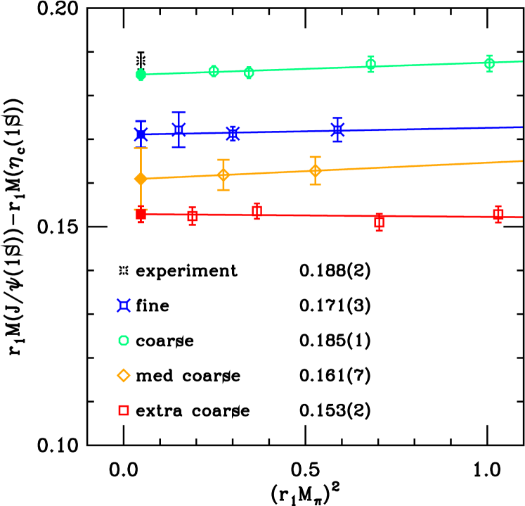
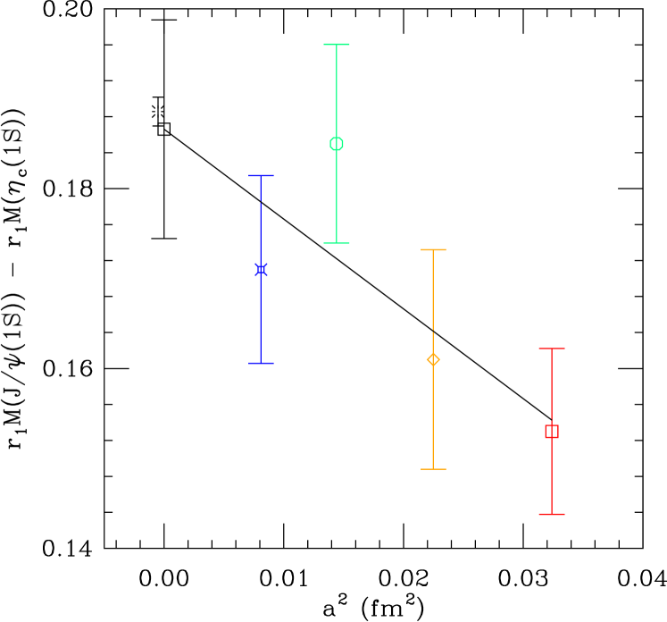
Figure 1: Results for charmonium hyperfine splitting. Splittings are in $r_{1}=0.318$ fm units. (1/$r_{1}=620$ MeV). The left panel shows the chiral extrapolation with only statistical errors shown. The right panel shows the continuum extrapolation in $a^{2}$ with kappa tuning errors of 6% included.

3.1 Charmonium hyperfine splitting

Hyperfine splitting provides a direct measure of the strength of the spin-spin chromomagnetic interaction. In Fig. 1 we show our results for charmonium hyperfine splitting. Here only the quark line “connected” diagrams are included. The dependence on sea quark mass is evidently quite weak. The continuum extrapolation, shown with kappa tuning errors included, gives 116(5) MeV compared with 117(1) MeV from experiment. It would clearly be good to reduce $\kappa$-tuning errors.

The contribution to the charmonium correlator and mass from quark line disconnected diagrams is expected to be small, so they are usually ignored. Because it is so small, it is a challenge to calculate it [9]. Our most recent results are given in Table 3. We find that annihilation processes actually decrease the magnitude of the splitting. The effect is smaller than or comparable to our current errors in the connected contribution.

superfine	0.06 fm	$-3.4(3)$ MeV
fine	0.09 fm	$-5.5(8)$ MeV

Table 3: Contribution from charm annihilation to the charmonium hyperfine splitting

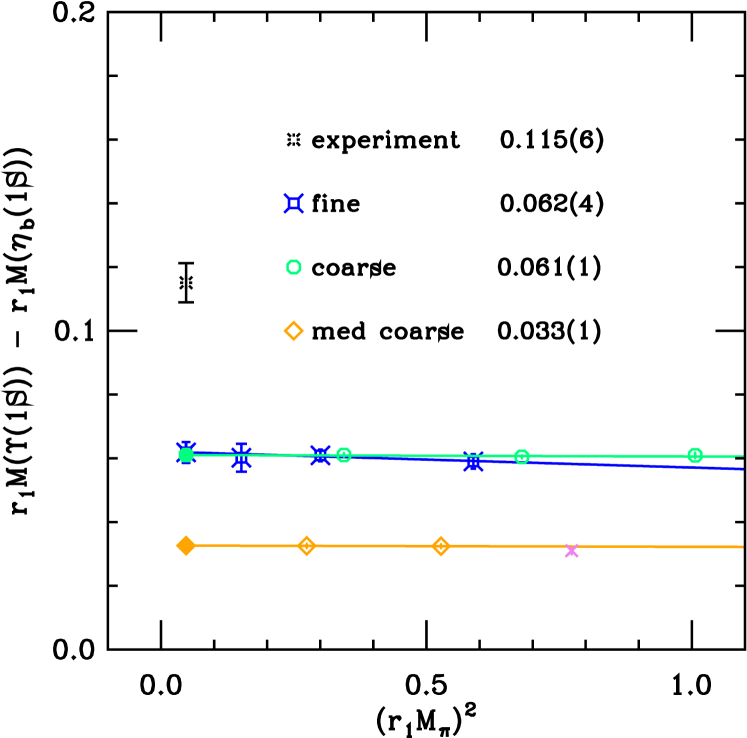
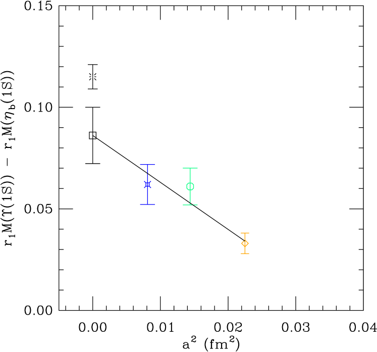
Figure 2: The left panel shows the chiral extrapolation with only statistical errors shown. The right panel shows the continuum extrapolation in $a^{2}$ with kappa tuning errors of 15% included, resulting in 53(9) MeV.

3.2 Bottomonium hyperfine splitting

In Fig. 2 we show results for hyperfine splitting of the bottomonium ground state. The continuum extrapolation gives 53(8) MeV. The $\eta_{b}$ was recently found [11, 12] with a splitting of 71(4) MeV from the $\Upsilon(1S)$. The HPQCD collaboration reports 61(4)(13) [13] using an NRQCD method with a chromomagnetic interaction of a quality comparable to ours.

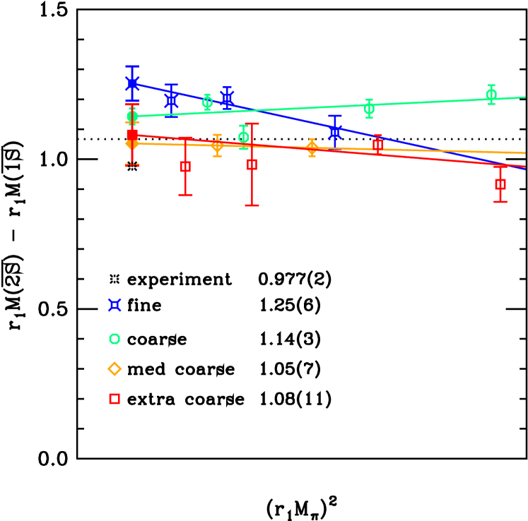
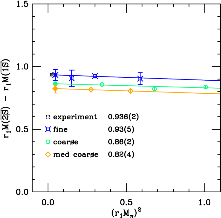
Figure 3: Splitting of the spin-averaged $2S$ and $1S$ levels in charmonium (left) and bottomonium (right). The dashed line indicates the physical open charm threshold. Since the $\eta_{b}^{\prime}$ has not been observed the “experimental” point uses only the $\Upsilon(2S)$ in the splitting.

3.3 $2S-1S$ level splitting

In Fig. 3 we show results for the splitting of the spin-averaged $\bm{\overline{2S}}$ and $\bm{\overline{1S}}$ levels. This quantity tests the “central” part of the quarkonium effective potential. We see that agreement with experiment in the charmonium case is not good. It is better in the bottomonium case. Our fit model does not include open charm states. So the $2S$ charmonium state could be confused with the nearby open charm threshold that comes closer as the light sea quark mass decreases. The dashed line locates the physical open charm threshold. For the bottomonium case the open bottom threshold is safely off scale.

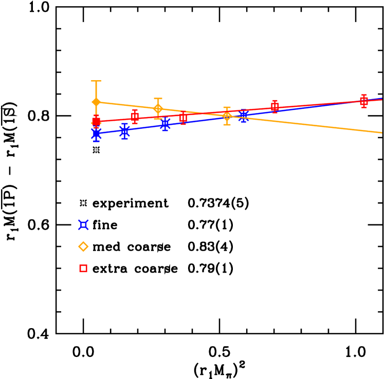
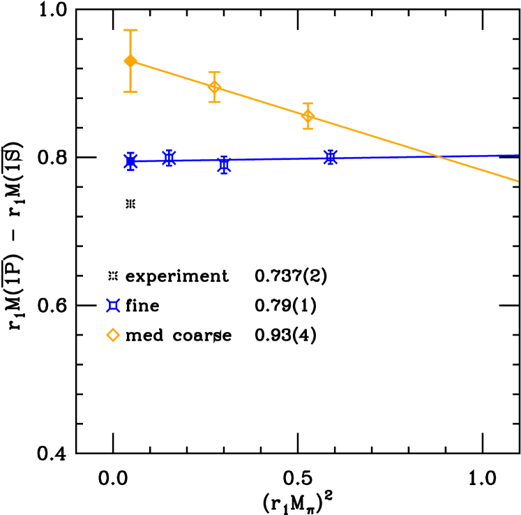
Figure 4: Splitting of the spin-averaged $1P$ and $1S$ levels in charmonium (left) and bottomonium (right).

3.4 $1P-1S$ splitting

The spin-averaged $\bm{\overline{1P}-\overline{1S}}$ splitting, shown in Fig. 4, also tests the central part of the potential. Within errors, our results seem to approach the experimental value.

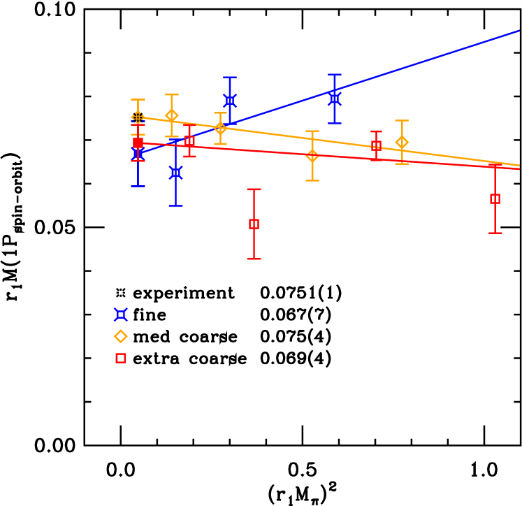
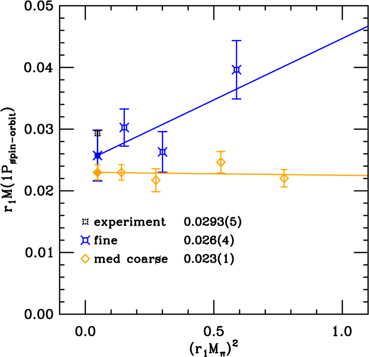
Figure 5: Spin-orbit combination from the $1P$ levels for charmonium (left) and bottomonium (right).

3.5 Spin-orbit and tensor components

The contribution to the $J=0$, 1, and 2 P-wave masses from the spin-orbit term in the quarkonium effective potential can be isolated with the combination

$$m_{1P_{\rm spin-orbit}}={\textstyle\frac{1}{9}}\left(5m_{c2}-2m_{c0}-3m_{c1}\right)$$

Our result is shown in Fig. 5. This term tests the strength of the chromoelectric interaction. In both cases the results seem to approach the experimental value in the chiral and continuum limits.

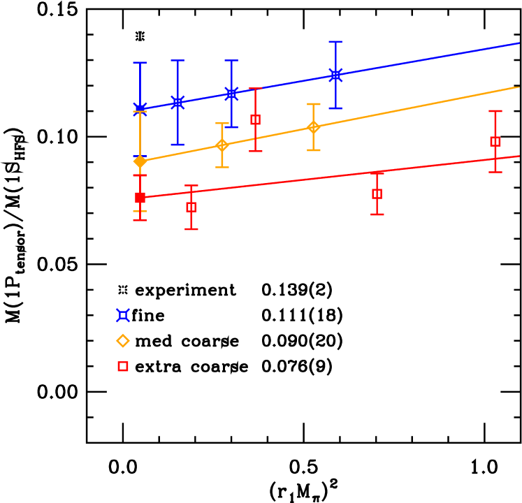
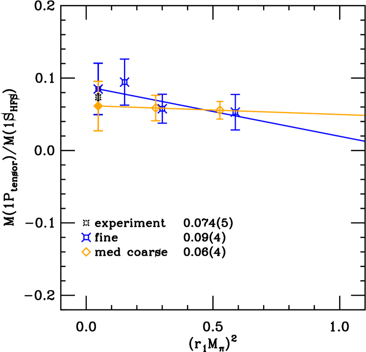
Figure 6: The $1P$ tensor combination, divided by the $1S$ hyperfine splitting for charmonium (left) and bottomonium (right).

Similarly, the contribution to the P-wave levels from the tensor component is proportional to the combination

$$m_{1P_{\rm tensor}}={\textstyle\frac{1}{9}}\left(3m_{c1}-m_{c2}-2m_{c0}\right),$$

shown in Fig. 6. Since the tensor and spin-spin components both measure the strength of the chromomagnetic interaction, here we divide by the 1S hyperfine splitting to see whether they are proportional. It appears that they are not. Still the results seem to approach the experimental values in the chiral and continuum limits.

3.6 Full spectrum

In Fig. 7 we reconstruct the low-lying quarkonium spectrum from splittings, starting from the experimental value for the spin-averaged $1S$ level.

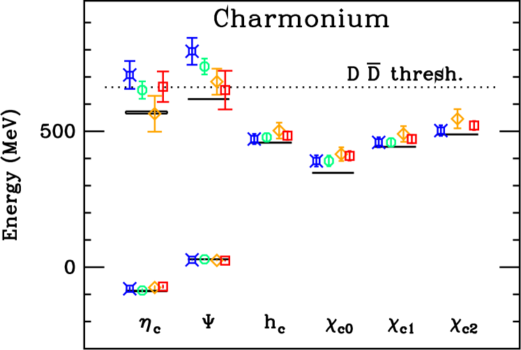
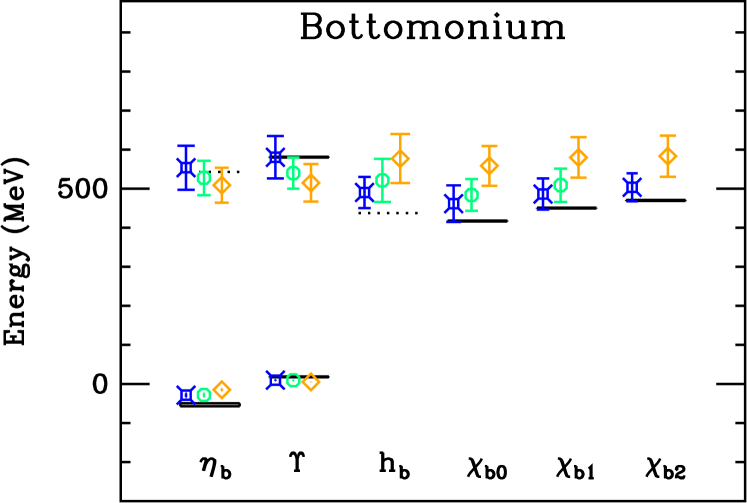
Figure 7: All quarkonium levels in this study, constructed from splittings from the physical $\overline{1S}$ level for charmonium (left) and bottomonium (right). Error bars include kappa tuning errors. Symbol colors distinguish the lattice spacings: 0.18 fm (red), 0.15 fm (orange), 0.12 fm (green), 0.09 fm (blue)

4 Conclusion and Outlook

We have seen that in most cases quarkonium level splittings are quite insensitive to the light sea quark masses. Systematic uncertainties in tuning the quark masses are much larger than our statistical errors. With the present set of lattice spacings and the present level of precision, the Fermilab action seems to perform well in the charmonium system, but there are indications that lattice discretization artifacts affect some of our bottomonium splittings. Work currently underway seeks a more precise determination of the charm and bottom masses and will use the still finer MILC-collaboration $0.06$ fm lattices.

- [1] M. Di Pierro et al., Nucl. Phys. Proc. Suppl. 119, 586 (2003) [arXiv:hep-lat/0210051]; Nucl. Phys. Proc. Suppl. 129, 340 (2004) [arXiv:hep-lat/0310042]; S. Gottlieb et al., \posPoS(LAT2005)203 (2006) [arXiv:hep-lat/0510072]; \posPoS(LAT2006)175 (2006) [arXiv:0910.0048 [hep-lat]].
- [2] C. Bernard et al. [Fermilab Lattice and MILC Collaborations], in preparation (2009).
- [3] C. W. Bernard et al., Phys. Rev. D 64, 054506 (2001) [arXiv:hep-lat/0104002].
- [4] C. Aubin et al., Phys. Rev. D 70, 094505 (2004) [arXiv:hep-lat/0402030].
- [5] A. Bazavov et al. [MILC collaboration], Rev. Mod. Phys. (to be published) [arXiv:0903.3598].
- [6] A. X. El-Khadra, A. S. Kronfeld and P. B. Mackenzie, Phys. Rev. D 55, 3933 (1997) [arXiv:hep-lat/9604004].
- [7] T. Burch et al. [Fermilab Lattice and MILC Collaborations], in preparation (2009).
- [8] A. S. Kronfeld, Nucl. Phys. Proc. Suppl. 53, 401 (1997) [arXiv:hep-lat/9608139].
- [9] L. Levkova and C. E. DeTar, \posPoS(LATTICE 2008)133 [arXiv:0809.5086] and work in preparation (2009).
- [10] Y. Chen et al., Phys. Rev. D 73, 014516 (2006) [arXiv:hep-lat/0510074].
- [11] B. Aubert et al. [BaBar Collaboration], Phys. Rev. Lett. 101, 071801 (2008), [arXiv:0807.1086].
- [12] B. Aubert et al. [BaBar Collaboration], [arXiv:0903.1124].
- [13] A. Gray et al. [HPQCD Collaboration], Phys. Rev. D 72, 094507 (2005) [arXiv:hep-lat/0507013].