Evolutionary Dynamics of Populations with Conflicting Interactions:
Classification and Analytical Treatment Considering Asymmetry and Power

Abstract

Evolutionary game theory has been successfully used to investigate the dynamics of systems, in which many entities have competitive interactions. From a physics point of view, it is interesting to study conditions under which a coordination or cooperation of interacting entities will occur, be it spins, particles, bacteria, animals, or humans. Here, we analyze the case, where the entities are heterogeneous, particularly the case of two populations with conflicting interactions and two possible states. For such systems, explicit mathematical formulas will be determined for the stationary solutions and the associated eigenvalues, which determine their stability. In this way, four different types of system dynamics can be classified, and the various kinds of phase transitions between them will be discussed. While these results are interesting from a physics point of view, they are also relevant for social, economic, and biological systems, as they allow one to understand conditions for (1) the breakdown of cooperation, (2) the coexistence of different behaviors (“subcultures”), (3) the evolution of commonly shared behaviors (“norms”), and (4) the occurence of polarization or conflict. We point out that norms have a similar function in social systems that forces have in physics.

I Introduction

Game theory is a theory of interactions, which goes back to von Neumann Neumann , one of the superminds of quantum mechanics. It is is based on mathematical analyses gamedyn0 ; Weibull ; Cressman ; NowBook and methods from statistical physics and the theory of complex systems HelGame ; minority ; Roca ; cyclic ; Claus , while applications range from biology gamedyn0 ; NowBook over sociology Axelrod1 ; gamedyn3 ; Skyrms ; Boyd ; Bounds to economics Neumann ; Bounds ; Binmore ; Henrich . Physicists have been particularly interested in evolutionary game theory gamedyn0 ; Weibull ; Cressman ; gamedyn3 ; exploratory , which focuses on the dynamics resulting from the interactions among a large number of entities. These could, for example, be spins, particles, bacteria, animals, or human beings. For such systems, one can calculate the statistical distribution of states in which the entities can be. These states reflect, for example, the location in space NJP ; EPL and/or whether a spin is oriented “up” or “down” RandomReplicators ; Preprint , while in non-physical systems, the states represent decisions, behaviors, or strategies. In such a way, one can study problems ranging from the spontaneous magnetization in spin glasses RandomReplicators ; Preprint up to the emergence of behavioral conventions HelGame ; Mueller ; Peyton . Further application areas are nucleation processes Schweitz1 ; Schweitz2 , the theory of evolution Eigen ; Fisher ; Ebeling ; gamedyn0 , predator-prey systems Hofbauer ; Montroll and the stability of ecosystems Montroll ; MayBook ; Diversity ; ReplicatorEcosyst3 . Physicists have also been interested in the effects of spatial interactions Space ; Space2 ; PhysLife or network interactions Network2 ; networkSW ; coevol ; Zhong ; network ; Ohtsuki ; Communities ; Szolnoki , of mobility Frey ; NJP ; HelPlat ; HelACS ; HelEPJB ; EPL ; HelPNAS or perturbations EPL ; HelPNAS ; Perc ; Noise2 ; Noise3 .

Recently, particular attention has been paid to the emergence of cooperation in dilemma situations NowBook ; Five , which are reflected by a number of different games charactarized by different types of interactions Weibull : In the stag hunt game (SH), cooperation is risky, in the snowdrift game (SD), free-riding (“defection”) is tempting, while both problems occur in the prisoner’s dilemma (PD) PhysLife . Details will be discussed in Sec. IV.2. Most of the related studies have assumed homogeneous populations so far (where every entity has the same kind of interactions). Here, we will study the heterogeneous case with multiple interacting populations. Compared to previous contributions for multiple populations Mueller ; SelfInt ; Weibull ; Arga ; Kana2 , we will focus on populations with conflicting interests and different power. Furthermore, we will classify the possible dynamical outcomes, and discuss the phase transitions when model parameters cross certain critical thresholds (“tipping points”).

Our paper is structured as follows: Section II introduces the game-dynamical replicator equations for multiple interacting populations. Afterwards, Sec. II.1 specifies the payoff matrices representing conflicting interactions. While doing so, we will take into account the (potentially different) power of populations. Then, Sec. III derives the stationary solutions of the evolutionary equations and the associated eigenvalues, which determine the instability properties of the stationary solutions. This is the basis of our classification. Section IV collects and discusses the main results regarding the dynamics of the system and possible phase transitions when model parameters are changing. It also offers an interpretation of the formal theory. Finally, Sec. V presents a summary and outlook.

II Game-Dynamical Replicator Equations for Interacting Populations

In the following, we will formulate game-dynamical equations for multi-population interactions Mueller ; SelfInt ; Weibull ; Arga ; Kana2 . For this, we will distinguish different (sub-)populations $a,b,c\in\{1,\dots,\mathcal{A}\}$ and various states (behaviors, strategies) $i,j,k\in\{1,\dots,I\}$. If an entity of population $a$ characterized by state $i$ interacts with an entity of population $b$ characterized by state $j$, the outcome (“success”) of the interaction is quantified by the “payoff” $A_{ij}^{ab}$. Now, let $f_{a}\geq 0$ with $\sum_{a}f_{a}=1$ be the fraction of entities belonging to population $a$ and $p_{i}^{a}(t)\geq 0$ with $\sum_{i}p_{i}^{a}(t)=1$ the proportion of entities in population $a$ characterized by state $i$ at time $t$. We will assume that entities take over (copy, imitate) states that are more successful in their population in accordance with the proportional imitation rule Mueller ; Schlag . Moreover, when the interaction frequency with entities of population $b$ characterized by state $j$ is $f_{b}p_{j}^{b}$ (i.e. proportional to the relative size or “power” $f_{b}$ of that population and the relative frequency $p_{j}^{b}$ of state $j$ in it), we find the following set of coupled game-dynamical equations Mueller :

$$\frac{dp_{i}^{a}(t)}{dt}=p_{i}^{a}(t)\big{[}E_{i}^{a}(t)-A_{a}(t)\big{]}\,.$$ (1)

Herein, the “expected success”

$$E_{i}^{a}(t)=\sum_{b=1}^{\mathcal{A}}\sum_{j=1}^{I}A_{ij}^{ab}f_{b}p_{j}^{b}(t)$$ (2)

of entities belonging to population $a$ characterized by state $i$ is obtained by summing up the payoffs $A_{ij}^{ab}$ over all possible states $j$ of interaction partners and populations $b$, weighting the payoffs with the respective occurrence frequencies $f_{b}p_{j}^{b}(t)$. (Note that $\sum_{b}\sum_{j}f_{b}p_{j}^{b}(t)=1$.) The quantity

$$A_{a}(t)=\sum_{k=1}^{I}p_{k}^{a}(t)E_{k}^{a}(t)$$ (3)

is the average success in population $a$ and

$$\langle A\rangle=\sum_{a=1}^{\mathcal{A}}f_{a}A_{a}(t)$$ (4)

the average success in all populations. The above game-dynamical equations assume that population sizes (and the population an entity belongs to) do not change.

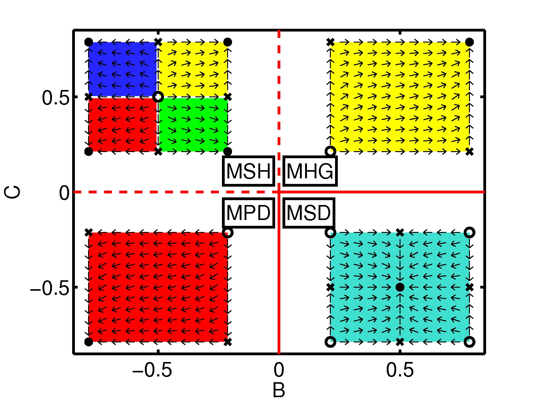
Figure 1: (Color Online) Illustration of the outcomes of symmetrical $2\times 2$ games as a function of the payoff-dependent parameters $b_{a}=B$ and $c_{a}=C$, if $f=0.8$ (i.e. 80% of individuals belong to population 1) and if the entities interact within their own population, but different populations do not have any interactions between each other ($B_{a}=0=C_{a}$) Weibull ; Preprint . $p=p_{1}^{1}$ is the fraction of entities of population 1 in state 1 and $q=p_{2}^{2}$ the fraction of entities of population 2 in state 2. The vector fields show $(dp/dt,dq/dt)$, i.e. the direction and size of the expected change of the distribution $(p,q)$ of states with time $t$. Sample trajectories illustrate some representative flow lines $(p(t),q(t))$ as time $t$ passes. The flow lines move away from unstable stationary points (empty circles). Saddle points (crosses) are attractive in one direction, but repulsive in another. Stable stationary points (black circles) attract the flow lines from all directions. Each color (grey shade) represents one basin of attraction. It subsumes all initial conditions $(p(0),q(0))$ leading to the same stationary point [yellow = (1,1), green = (1,0), blue = (0,1), red = (0,0), turquoise = $(p_{0},p_{0})$ with $p_{0}=|B|/(|B|+|C|)$]. Solid red lines indicate the thresholds at which continuous (“second-order”) phase transitions take place, i.e. at which the system behavior changes qualitatively (characterized by the appearance or disappearance of stationary points), while the stable stationary points change continuously when the parameters are varied. Dashed lines indicate an abrupt change of a stable stationary point, i.e. a discontinous (“first-order”) phase transition. For multi-population prisoner’s dilemmas (MPD), we have $B<0$ and $C<0$, and the final outcome is $(p,q)=(0,0)$. For multi-population snowdrift games (MSD), we have $B>0$ and $C<0$, and the stable stationary solution corresponds to a coexistence of a fraction $p_{0}=|B|/(|B|+|C|)$ of entities in one state and a fraction $1-p_{0}$ of entities in the other. For multi-population harmony games (MHG), we have $B>0$ and $C>0$, and the eventually resulting outcome is (1,1). Finally, for multi-population stag hunt games (MSH), we have $B<0$ and $C>0$, and there is a bistable situation, i.e. it depends on the initial fraction of entities in a state, whether everybody ends up in this state or in the other one Preprint .

Comparing the above game-dynamical equations with the usual replicator equation for the one-population case, we have additional terms involving payoffs $A_{ij}^{ab}$ from interactions with different populations $b\neq a$. They lead to a mutual coupling of the replicator equations (1). Asymmetrical games with different payoff matrices of the interacting entities, or games between entities with different sets of states (strategy sets) are examples for the need to distinguish between different populations. Within the framework of game-dynamical equations they can be treated as bimatrix games Weibull ; gamedyn0 ; Cressman . These, however, do not consider interactions among entities belonging to the same population (“self-interactions”), which are reflected by the payoff matrices $A_{ij}^{aa}$. The above multi-population replicator equations include interactions both within the same population and between different populations. The significantly different dynamics and outcomes when interactions between two populations are neglected or when self-interactions are neglected become obvious when Figs. 1 and 2 are compared with Fig. 3.

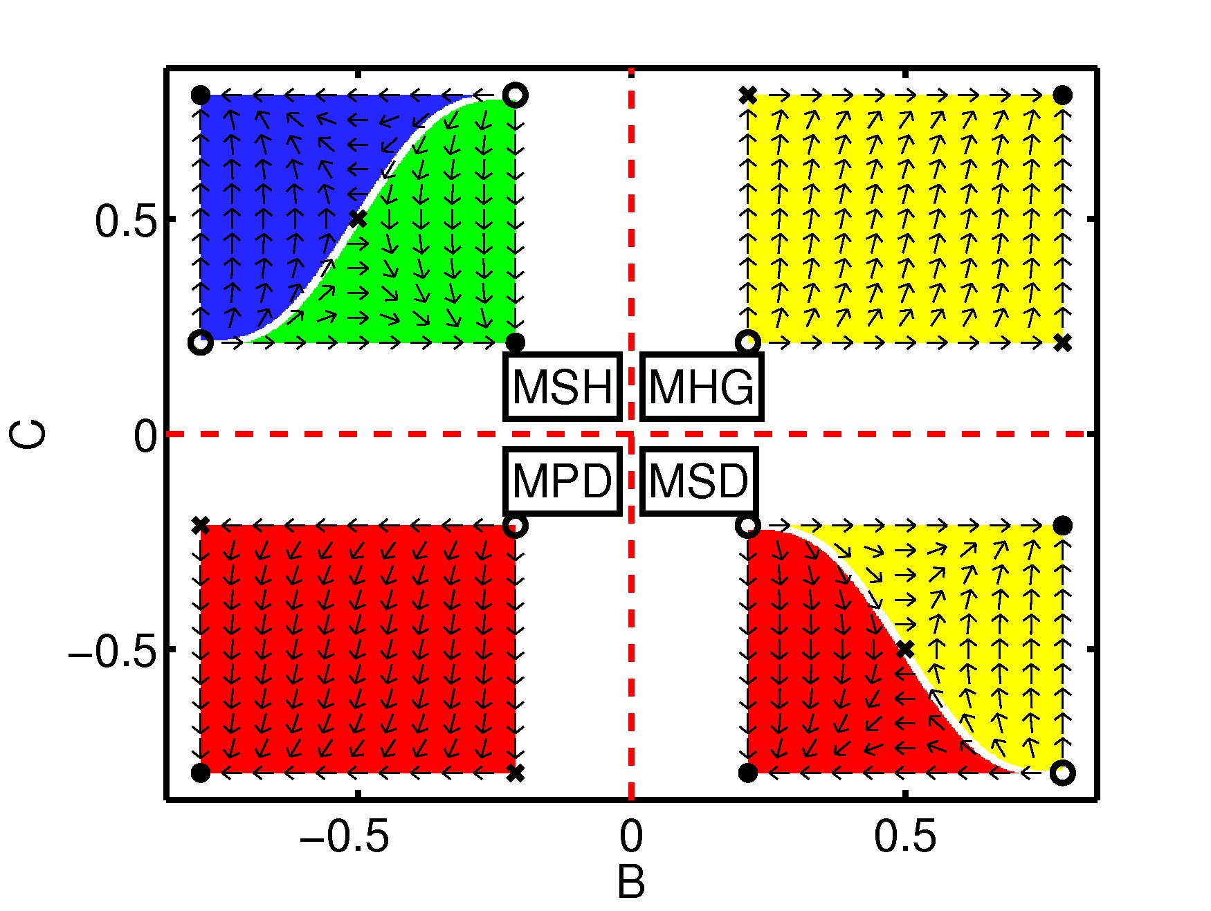
Figure 2: (Color Online) Illustration of the outcomes as a function of the payoff-dependent parameters $B_{a}=B$ and $C_{a}=C$, if $f=0.8$ (i.e. 80% of the entities belong to population 1) and if the entities do not interact within their own population ($b_{a}=0=c_{a}$), while entities belonging to different populations have interactions with each other Weibull . Small arrows illustrate again the vector field $(dp/dt,dq/dt)$ as a function of $p=p_{1}^{1}$ and $q=p_{2}^{2}$. Black circles represent stable fix points, empty circles stand for unstable fix points, and crosses represent saddle points. The basins of attraction of different stable fix points are represented in different grey shades (colors) [yellow = (1,1), green = (1,0), blue = (0,1), red = (0,0)]. Solid red lines indicate the thresholds at which continuous phase transitions take place, dashed lines indicate discontinous phase transitions. For multi-population prisoner’s dilemmas (MPD), we have $B<0$ and $C<0$, for multi-population snowdrift games (MSD), we have $B>0$ and $C<0$, for multi-population harmony games (MHG), we have $B>0$ and $C>0$, and for the multi-population stag hunt game (MSH), we have $B<0$ and $C>0$.

For reasons of simplicity and analytical tractability, we will now focus on the case of two populations ($\mathcal{A}=2$) with two states each ($I=2$). This allows one to reduce the number of variables by means of the normalization conditions $f_{1}=1-f_{2}$, $p_{2}^{1}(t)=1-p_{1}^{1}(t)$ and $p_{1}^{2}(t)=1-p_{2}^{2}(t)$. Furthermore, we find

$$E_{1}^{1}(t)-A_{1}(t) = E_{1}^{1}(t)-p_{1}^{1}(t)E_{1}^{1}(t)-[1-p_{1}^{1}(t)]E_{2}^{1}(t)$$ (5)

$$= [1-p_{1}^{1}(t)][E_{1}^{1}(t)-E_{2}^{1}(t)]\,.$$

When evaluating the expected success $E_{i}^{a}(t)$, we will write the payoff matrices $A_{ij}^{ab}$ for population $a=1$ as

$$(A_{ij}^{11})=\left(\begin{array}[]{cc}r_{1}&s_{1}\\ t_{1}&p_{1}\end{array}\right)\quad\mbox{and}\quad(A_{ij}^{12})=\left(\begin{array}[]{cc}R_{1}&S_{1}\\ T_{1}&P_{1}\end{array}\right)\,.$$ (6)

II.1 Specification of Conflicting Interactions

To reflect conflicting interactions, the payoffs in population $a=2$ are assumed to be inverted (“mirrored”), i.e. state 2 plays the role in population 2 that state 1 plays in population 1:

$$(A_{ij}^{21})=\left(\begin{array}[]{cc}P_{2}&T_{2}\\ S_{2}&R_{2}\end{array}\right)\quad\mbox{and}\quad(A_{ij}^{22})=\left(\begin{array}[]{cc}p_{2}&t_{2}\\ s_{2}&r_{2}\end{array}\right)\,.$$ (7)

With the abbreviations $p(t)=p_{1}^{1}(t)$ and $q(t)=p_{2}^{2}(t)$, this leads to

$$E_{1}^{1}(t) = r_{1}fp(t)+s_{1}f[1-p(t)]$$ (8)

$$+ R_{1}(1-f)[1-q(t)]+S_{1}(1-f)q(t)$$

and

$$E_{2}^{1}(t) = t_{1}fp(t)+p_{1}f[1-p(t)]$$ (9)

$$+ T_{1}(1-f)[1-q(t)]+P(1-f)q(t)\,.$$

The parameter $f=f_{1}$ represents the (relative) power of population 1, and $(1-f)=f_{2}$ the power of population 2. Inserting Eqs. (8) and (9) into Eqs. (5) and (1), the game-dynamical equation for population 1 becomes

$$\frac{dp(t)}{dt}=\underbrace{p(t)[1-p(t)]}_{\rm saturation\ factors}\underbrace{F\big{(}p(t),q(t)\big{)}}_{\rm growth\ factor}$$ (10)

with $F(p,q)=E_{1}^{1}-E_{2}^{1}$. Explicitly, we have

$$F(p,q)=b_{1}f+(c_{1}-b_{1})fp+C_{1}(1-f)+(B_{1}-C_{1})(1-f)q\,,$$ (11)

where

$$b_{1}=s_{1}-p_{1},\mbox{ \ }c_{1}=r_{1}-t_{1},\mbox{ \ }B_{1}=S_{1}-P_{1},\mbox{ \ }C_{1}=R_{1}-T_{1}\,.$$ (12)

The supplementary equation for population 2 reads

$$\frac{dq(t)}{dt}=\underbrace{q(t)[1-q(t)]}_{\rm saturation\ factors}\underbrace{G\big{(}p(t),q(t)\big{)}}_{\rm growth\ factor}$$ (13)

with

$$G(p,q)=b_{2}(1-f)+(c_{2}-b_{2})(1-f)q+C_{2}f+(B_{2}-C_{2})fp\,.$$ (14)

It is obtained by exchanging $p$ and $q$, $f$ and $1-f$, and indices $1$ and $2$. The first factors may be interpreted as saturation factors, as they limit the proportions $p$ and $q$ to the admissible range from 0 to 1. The factors $F(p,q)$ and $G(p,q)$ can be interpreted as growth factors, if greater than zero (or as decay factors, if smaller than zero). Note that the above two-population game-dynamical equations are general enough to capture all possible $2\times 2$ games and even situations when entities of different populations play different kinds of games (“asymmetrical” case).

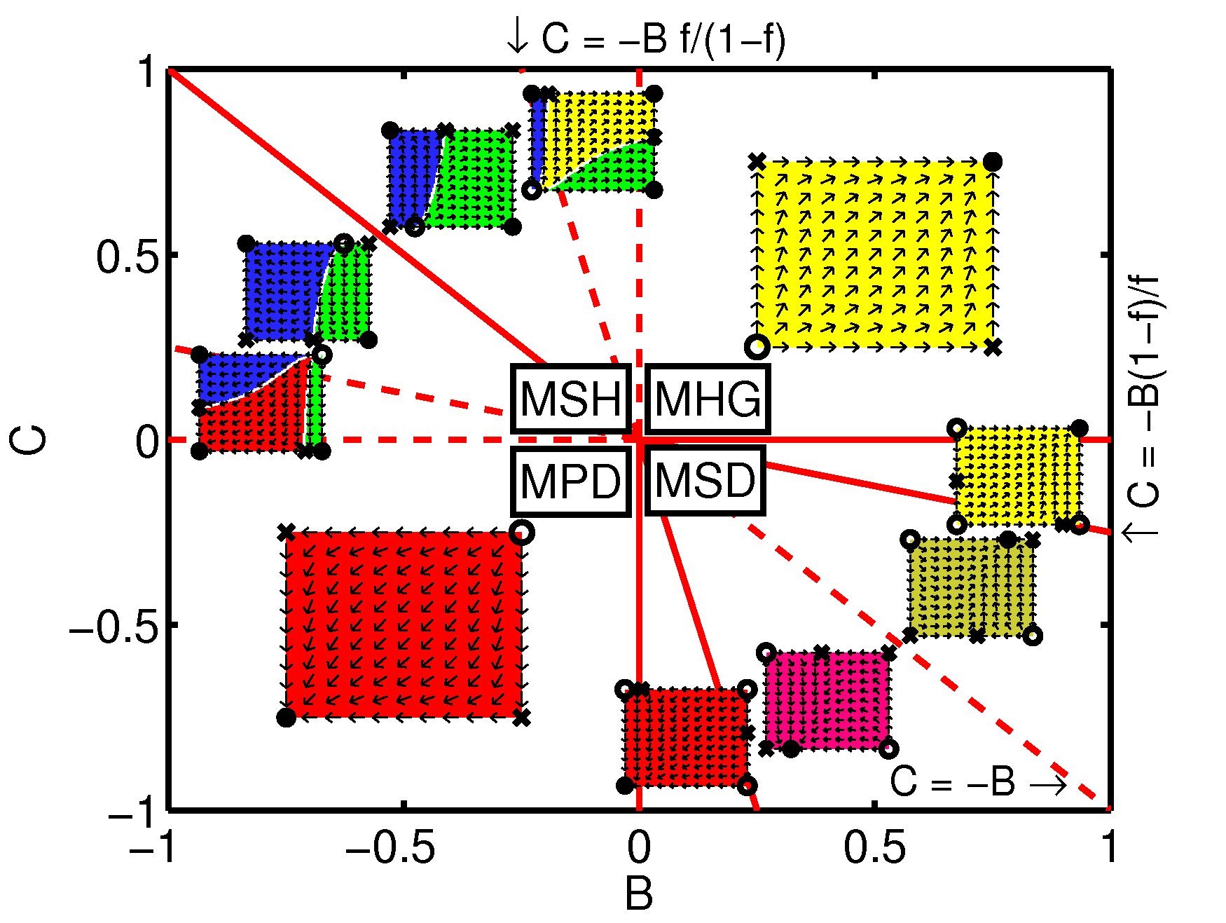
Figure 3: (Color Online) Illustration of the parameter-dependent types of outcomes as a function of the payoff-dependent parameters $B_{a}=b_{a}=B$ and $C_{a}=c_{a}=C$, if $f=0.8$ (i.e. 80% of the entities belong to population 1) and if the entities have interactions with other entities, independently of the population they belong to. This corresponds to the multi-population case with interactions and self-interactions. Small arrows illustrate the vector field $(dp/dt,dq/dt)$ as a function of $p$ and $q$. Empty circles stand for unstable fix points (repelling neighboring trajetories), black circles represent stable fix points (attracting neighboring trajectories), and crosses represent saddle points (i.e. they are attractive in one direction and repulsive in the other). The basins of attraction of different stable fix points are represented in different shades of grey (colors) [red = (0,0), green = (1,0), blue = (0,1), yellow = (1,1), salmon = $(u,0)$, mustard = $(v,1)$, where $0<u,v<1$]. Solid red lines indicate the thresholds at which continuous phase transitions take place, dashed lines indicate discontinous phase transitions. For multi-population prisoner’s dilemmas (MPD), we have $B<0$ and $C<0$, for multi-population snowdrift games (MSD), we have $B>0$ and $C<0$, for multi-population harmony games (MHG), we have $B>0$ and $C>0$, and for the multi-population stag hunt game (MSH), we have $B<0$ and $C>0$.

II.2 Special Cases

If there are no interactions between entities of different populations, we have $B_{a}=0=C_{a}$. In that case, both populations separately behave as expected in the one-population case (see Fig. 1 and Movie 1 Movies ). Instead, if there are interactions between both populations, but no self-interactions, we have $b_{a}=0=c_{a}$. In that situation, we end up with conventional bimatrix games (see Fig. 2 and Movie 2 Movies ). In the following, we will assume that everyone has interactions with entities of all populations with a frequency that is proportional to the relative population sizes. For simplicity, we will furthermore focus on the case where the payoffs depends only on the state, but not the population of the interaction partner. Then, we have $p_{a}=P_{a}=P$, $r_{a}=R_{a}=R$, $s_{a}=S_{a}=S$, and $t_{a}=T_{a}=T$, i.e.

$$b_{a}=B_{a}=B=S-P$$ (15)

and

$$c_{a}=C_{a}=C=R-T$$ (16)

(see Fig. 3 and Movie 3 Movies ). If the interaction rate between different populations is $\nu$ times the interaction rate within the own population, we have the more general relationship $B_{a}=\nu b_{a}=\nu B$ and $C_{a}=\nu c_{a}=\nu C$ (where the parameter $\nu>0$ allows us to tune the interaction frequency between two populations—until now, we have assumed $\nu=1$). In that case, we obtain

$$F(p,q)=F_{\nu}(p,q) = B\underbrace{[f(1-p)+\nu(1-f)q]}_{\geq 0}$$ (17)

$$+ C\underbrace{[fp+\nu(1-f)(1-q)]}_{\geq 0}\quad$$

and

$$G(p,q)=G_{\nu}(p,q) = B\underbrace{[(1-f)(1-q)+\nu fp]}_{\geq 0}$$ (18)

$$+ C\underbrace{[(1-f)q+\nu f(1-p)]}_{\geq 0}\,.\quad$$

Note that one can restrict the analysis of the two-population game-dynamical equations to $f\geq 0.5$, as the transformations $f\leftrightarrow(1-f)$ and $p\leftrightarrow q$ leave the two-population replicator equations unchanged.

III Stationary Solutions, Eigenvalues, and Possible System Dynamics

In the two-dimensional space defined by the variables $p$ and $q$, the qualitative properties of the vector field (which determines the temporal changes $dp/dt$ and $dq/dt$) can be completely derived from the stationary solutions and their stability properties, which are given by their eigenvalues. These can be calculated analytically, i.e. there are exact mathematical formulas for them.

III.1 Basic Definitions

For an interdisciplinary readership, we will shortly define some relevant terminology here, while specialists may directly continue with subsection B. A stationary solution $(p_{l},q_{l})$ is defined as a point with $dp/dt=0$ and $dq/dt=0$, which implies

$$p_{l}(1-p_{l})F(p_{l},q_{l})=0\quad\mbox{and}\quad q_{l}(1-q_{l})G(p_{l},q_{l})=0\,.$$ (19)

Besides calculating the stationary solutions, one may perform a so-called “linear stability analysis”, which allows one to find out how a solution

$$(p(t),q(t))=(p_{l}+\delta p_{l}(t),q_{l}+\delta q_{l}(t))$$ (20)

in the vicinity of a stationary solution $(p_{l},q_{l})$ evolves in time. If the distance

$$d_{l}(t)=\sqrt{\delta p_{l}(t)^{2}+\delta q_{l}(t)^{2}}$$ (21)

goes to zero, which may be imagined as an attraction towards the stationary solution, one speaks of a stable stationary point or an asymptotically stable fix point or an evolutionary equilibrium gamedyn3 (which is a so-called Nash equilibrium). Its basin of attraction is defined by the set of all initial conditions $(p(0),q(0))$, for which the trajectories $(p(t),q(t))$ starting in these points end up in the fix point under consideration as time $t$ goes to infinity. (In Figs. 1–5 and Movies 1–3 Movies , they are represented by different background colors.)

If the distance $d_{l}(t)$ grows rather than shrinks with time $t$, one speaks of an unstable fix point. This may be imagined like a repulsion from the stationary solution. If the growth or shrinkage of the distance $d_{l}$ is a matter of the specific choice of the initial conditions $p(0)=p_{l}+\delta p_{l}(0)$ and $q(0)=q_{l}+\delta q_{l}(t)$, the stationary point is called a saddle point. A saddle point is attractive in one direction, but repulsive in another one. In Figs. 1–5 and Movies 1–3 Movies , the stationary points and their respective stability properties (marked by circles and crosses) have been determined analytically. They fit perfectly to the numerically calculated vector fields, which represent $(dp/dt,dq/dt)$, i.e. the size and direction of changes in the distribution $(p,q)$ of states with time.

III.2 Calculation of the Stationary Solutions and their Eigenvalues

We will now identify the stationary solutions $(p_{l},q_{l})$ satisfying $dp/dt=0$ and $dq/dt=0$ and their respective eigenvalues $\lambda_{l}$ and $\mu_{l}$. Using the notation $p(t)=p_{l}+\delta p_{l}(t)$ and $q(t)=q_{l}+\delta q_{l}(t)$, the eigenvalues follow from the linearized equations

$$\frac{d}{dt}\left(\begin{array}[]{c}\delta p_{l}(t)\\ \delta q_{l}(t)\end{array}\right)=\left(\begin{array}[]{cc}M_{11}&M_{12}\\ M_{21}&M_{22}\end{array}\right)\left(\begin{array}[]{c}\delta p_{l}(t)\\ \delta q_{l}(t)\end{array}\right)$$ (22)

with

$$M_{11} = (1-2p_{l})F(p_{l},q_{l})+p_{l}(1-p_{l})(c_{1}-b_{1})f\,,$$

$$M_{12} = p_{l}(1-p_{l})(B_{1}-C_{1})(1-f)\,,$$

$$M_{21} = q_{l}(1-q_{l})(B_{2}-C_{2})f\,,$$ (23)

$$M_{22} = (1-2q_{l})G(p_{l},q_{l})+q_{l}(1-q_{l})(c_{2}-b_{2})(1-f)\,.$$

As the eigenvalue analysis of linear systems of differential equations is a standard procedure gamedyn3 , we will not explain it here in detail. We just note that the eigenvalues $\lambda_{l}$ and $\mu_{l}$ of a stationary point $(p_{l},q_{l})$ are given by the two solutions of the so-called characteristic polynomial

$$(M_{11}-\lambda_{l})(M_{22}-\mu_{l})-M_{12}M_{21}=0\,.$$ (24)

For the four stationary points $(p_{l},q_{l})$ with $l\in\{1,2,3,4\}$ discussed below, we have $p_{l},q_{l}\in\{0,1\}$, which implies $M_{12}M_{21}=0$. Therefore, the first associated eigenvalue is just

$$\lambda_{l}=M_{11}=(1-2p_{l})F(p_{l},q_{l})\,,$$ (25)

and the second associated eigenvalue is

$$\mu_{l}=M_{22}=(1-2q_{l})G(p_{l},q_{l})\,.$$ (26)

The following paragraph is again written for an interdisciplinary readership, while specialists may skip it. If both eigenvalues are negative, the corresponding stationary point $(p_{l},q_{l})$ is a stable fix point, i.e. “trajectories” $(p(t),q(t))$ in the neighborhood (flow lines) are attracted to it in the course of time $t$. If $\lambda_{l}$ and $\mu_{l}$ are both positive, the stationary solution will be an unstable fix point, and close-by trajectories will be repelled from it. If one eigenvalue is negative and the other one is positive, closeby trajectories are attracted in one direction, while they are repelled in another direction. This corresponds to a saddle point. If both eigenvalues are positive, closeby trajectories are repelled from the stationary solution. That situation is called an unstable fix point.

Let us now turn to the discussion of the stationary solutions of Eqs. (10) and (13) with the specifications (11) and (14):

• For the stationary solution $(p_{1},q_{1})=(0,0)$, we have the associated eigenvalues $\lambda_{1}=b_{1}f+C_{1}(1-f)$ and $\mu_{1}=b_{2}(1-f)+C_{2}f$.

• The point $(p_{2},q_{2})=(1,1)$ is also a stationary solution and has the eigenvalues $\lambda_{2}=-[c_{1}f+B_{1}(1-f)]$ and $\mu_{2}=-[c_{2}(1-f)+B_{2}f]$.

• The stationary solutions $(p_{3},q_{3})=(1,0)$ and $(p_{4},q_{4})=(0,1)$ exist as well. They have the eigenvalues $\lambda_{3}=-[c_{1}f+C_{1}(1-f)]$, $\mu_{3}=b_{2}(1-f)+B_{2}f$ and $\lambda_{4}=b_{1}f+B_{1}(1-f)$, $\mu_{4}=-[c_{2}(1-f)+C_{2}f]$.

• If $0\leq p_{k}\leq 1$ and $0\leq q_{k}\leq 1$ with

  $$p_{5} = \frac{b_{1}f+C_{1}(1-f)}{(b_{1}-c_{1})f}\,,$$ (27)

  $$p_{6} = \frac{b_{1}f+B_{1}(1-f)}{(b_{1}-c_{1})f}\,,$$ (28)

  $$q_{7} = \frac{b_{2}(1-f)+B_{2}f}{(b_{2}-c_{2})(1-f)}\,,$$ (29)

  $$q_{8} = \frac{b_{2}(1-f)+C_{2}f}{(b_{2}-c_{2})(1-f)}\,,$$ (30)

  we additionally have stationary points $(p_{5},q_{5})=(p_{5},0)$ with $F(p_{5},0)=0$, $(p_{6},q_{6})=(p_{6},1)$ with $F(p_{6},1)=0$, $(p_{7},q_{7})=(1,q_{7})$ with $G(1,q_{7})=0$, and/or $(p_{8},q_{8})=(0,q_{8})$ with $G(0,q_{8})=0$. These have the associated eigenvalues

  $$\qquad\lambda_{5}=p_{5}(1-p_{5})(c_{1}-b_{1})f,\ \mu_{5}=G(p_{5},0)\,,$$ (31)

  $$\qquad\lambda_{6}=p_{6}(1-p_{6})(c_{1}-b_{1})f,\ \mu_{6}=-G(p_{6},1)\,,$$ (32)

  $$\quad\mbox{ \ \,}\lambda_{7}=-F(1,q_{7}),\ \mu_{7}=q_{7}(1-q_{7})(c_{2}-b_{2})(1-f)\,,$$ (33)

  $$\qquad\lambda_{8}=F(0,q_{8}),\ \mu_{8}=q_{8}(1-q_{8})(c_{2}-b_{2})(1-f)\,.$$ (34)

• Inner stationary points $(p_{9},q_{9})$ with $0<p_{9}<1$, $0<q_{9}<1$ can only exist, if $F(p_{9},q_{9})=0=G(p_{9},q_{9})$ can be satisfied.

III.3 Special Case of Homogeneous Parameters

Let us now focus on the case of homogeneous parameters given by $b_{a}=B_{a}=B$ and $c_{a}=C_{a}=C$. In this case, the condition $F(p_{9},q_{9})=0=G(p_{9},q_{9})$ for an inner point can only be fulfilled for $B+C=0$. If $B=-C$, one finds a line

$$q(p)=\frac{1/2+f(p-1)}{1-f}$$ (35)

of fix points, which are stable for $B>0$, but unstable for $B<0$. Otherwise, fix points are only possible on the boundaries with either $p$ or $q\in\{0,1\}$.

Evaluating the conditions $0\leq p_{l}\leq 1$ and $0\leq q_{l}\leq 1$ reveals the following:

• The stationary point $(p_{5},0)$ only exists for $C<0<B$ and $f\geq|C|/(B+|C|)$ or for $B<0<C$ and $f\geq C/(|B|+C)$.

• $(p_{6},1)$ is a stationary point for $C<0<B$ and $f\geq B/(B+|C|)$ or for $B<0<C$ and $f\geq|B|/(|B|+C)$.

• The stationary point $(1,q_{7})$ only exists for $C<0<B$ and $f\leq|C|/(B+|C|)$ or for $B<0<C$ and $f\leq C/(|B|+C)$.

• $(0,q_{8})$ is a stationary point for $C<0<B$ and $f\leq B/(B+|C|)$ or for $B<0<C$ and $f\leq|B|/(|B|+C)$.

• If both, $B$ and $C$ are positive or negative at the same time, stationary points $(p_{l},q_{l})$ with $l\in\{5,\dots,8\}$ do not exist.

IV Overview of Main Results

For the special case with $b_{a}=B_{a}=B$ and $c_{a}=C_{a}=C$, our results depend on the type of game, the sizes $|B|$ and $|C|$ of the payoff-dependent model parameters, and the power $f$ of population 1 (e.g. its relative strength). They can be summarized as follows: For all values of the model parameters $B$, $C$, and $f$, all four corner points (0,0), (1,0), (0,1), and (1,1) are stationary solutions. However, if $B>0$ and $C>0$, the only asymptotically stable fix point is (1,1), while for $B<0$ and $C<0$, the only stable fix point is (0,0). In both cases, (1,0) and (0,1) are saddle points, and stationary points $(p_{l},q_{l})$ with $l\in\{5,...,8\}$ do not exist, as either the value of $p_{l}$ or of $q_{l}$ lies outside the range $[0,1]$, thereby violating the normalization conditions.

If $B<0$ and $C>0$, we have an equilibrium selection problem Preprint and find:

• (0,1) and (1,0) are always asymptotically stable fix points.

• (0,0) is a stable fix point for $|C|/|B|<\min[f/(1-f),(1-f)/f]$.

• (1,1) is a stable fix point for $|C|/|B|>\max[f/(1-f),(1-f)/f]$.

If $B>0$ and $C<0$ we have:

• (1,0) and (0,1) are always unstable fix points.

• (0,0) is a stable fix point for $|C|/|B|>\max[f/(1-f),(1-f)/f]$.

• (1,1) is a stable fix point for $|C|/|B|<\min[f/(1-f),(1-f)/f]$.

Moreover, if $B$ and $C$ have different signs, stationary points $(p_{l},q_{l})$ with $l\in\{5,...,8\}$ may occur:

• $(p_{5},0)$ is a fix point for $|C|/(|B|+|C|)\leq f$, i.e. $|C|/|B|\leq f/(1-f)$.

• $(p_{6},1)$ is a fix point for $|B|/(|B|+|C|)\leq f$, i.e. $|C|/|B|\geq(1-f)/f$.

• $(1,q_{7})$ is a fix point for $|C|/(B+|C|)\geq f$, i.e. $|C|/|B|\geq f/(1-f)$.

• $(0,q_{8})$ is a fix point for $|B|/(|B|+|C|)\geq f$, i.e. $|C|/|B|\leq(1-f)/f$.

IV.1 Phase Transitions Between Different Types of System Dynamics

It is natural that a change in the parameters $B$, $C$, and $f$ causes changes in the system dynamics. Normally, small parameter changes will imply smooth changes in the locations of fix points, their eigenvalues, the vector fields, and basins of attraction. However, when certain “critical” thresholds are crossed, new stable fix points may show up or disappear in remote places of the parameter space, which defines a discontinous (first-order) phase transition. If the locations of the stable fix points change continuously with a variation of the model parameters, while the related “dislocation speed” changes discontinously when crossing certain thresholds, we will talk of a second-order phase transition. In Figs. 1 to 5, continuous transitions are indicated by solid lines, while discontinous transitions are represented by dashed lines.

Analyzing the eigenvalues of the fix points (0,0), (1,0), (0,1), and (1,1), it is obvious that our model of two populations with conflicting interactions shows phase transitions, when $B$ or $C$ changes from positive to negative values or vice versa. The stationary point (0,0) is stable for $B<0$ and $C<0$, (1,0) and (0,1) are stable for $B<0$ and $C>0$, and (1,1) is stable for $B>0$ and $C>0$. This implies completely different types of system dynamics, and the transitions between these cases are discontinous (corresponding to first-order phase transitions). For $B>0$ and $C<0$, the stable fix point differs from the corner points (0,0), (1,0), (0,1), and (1,1), but its location changes continuously, as $B$ or $C$ crosses the zero line (corresponding to a second-order transition).

It is striking that conflicting interactions between two populations lead to further transitions, as $f$ or $|C|/|B|$ cross certain critical values: Namely, as $|C|$ is increased from 0 to high values, apart from (0,0), (0,1), (1,0), and (1,1), we find the following stationary points (given that $B$ and $C$ have different signs):

• $(p_{5},0)$ and $(0,q_{8})$, if $f\geq 1/2$ and $|C|/|B|\leq(1-f)/f$ or if $f\leq 1/2$ and $|C|/|B|\leq f/(1-f)$.

• $(p_{5},0)$ and $(p_{6},1)$, if $f\geq 1/2$ and $(1-f)/f<|C|/|B|<f/(1-f)$, or $(1,q_{7})$ and $(0,q_{8})$ if $f\leq 1/2$ and $f/(1-f)<|C|/|B|<(1-f)/f$.

• $(p_{6},1)$ and $(1,q_{7})$, if $f\geq 1/2$ and $|C|/|B|\geq f/(1-f)$ or if $f\leq 1/2$ and $|C|/|B|\geq(1-f)/f$.

For $B<0<C$, these fix points are unstable or saddle points, while they are stable or saddle points for $C<0<B$. When the equality sign in the above inequalities applies, fix points $(p_{l},q_{l})$ with $l\in\{5,6,7,8\}$ may become identical with (0,0), (0,1), (1,0), or (1,1).

Obviously, there are further transitions to a qualitatively different system behavior at the points $|C|/|B|=(1-f)/f$ and $|C|/|B|=f/(1-f)$ (see Figs. 3 to 5). These are continuous, if $B>0$ and $C<0$, but discontinuous for $B<0$ and $C>0$. Moreover, there is another transition, when $|C|$ crosses the value of $|B|$, as the stability properties of pairs of fix points are then interchanged (see Figs. 3–5 and Movie 3 Movies ). If $B<0$ and $C>0$, this transition is of second order, as the stable fix points remain unchanged as the model parameters are varied (see Fig. 4). However, for $B>0$ and $C<0$, the transition is discontinuous (i.e. of first order), because the stable fix point turns into an unstable one and vice versa (see Fig. 5). That can be followed from the fact that the dynamic system behavior and final outcome for the case $|B|>|C|$ can be derived from the results for $|B|<|C|$. This is done by applying the transformations $B\leftrightarrow-C$, $p\leftrightarrow(1-p)$, and $q\leftrightarrow(1-q)$, which do not change the game-dynamical equations

$$\frac{dp}{dt}=p(1-p)[Bf(1-p)+Cfp+C(1-f)(1-q)+B(1-f)q]$$ (36)

and

$$\frac{dq}{dt}=q(1-q)[B(1-f)(1-q)+C(1-f)q+Cf(1-p)+Bfp]\,.$$ (37)

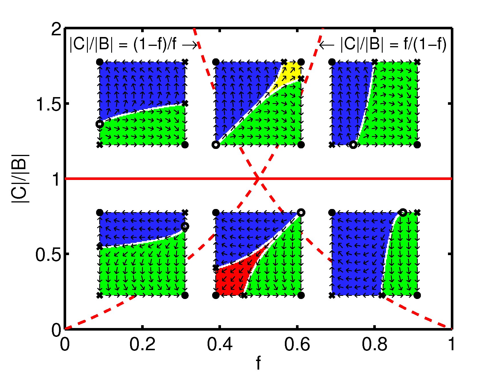
Figure 4: (Color Online) Illustration of the parameter-dependent types of outcomes in the multi-population stag-hunt game, if $|C|/|B|$ and/or $f$ are varied and interaction between populations as well as self-interactions are considered. The representation and grey shades (colors) are the same as in Fig. 3. Solid red lines indicate the thresholds at which continuous phase transitions take place, dashed lines indicate discontinous phase transitions.

IV.2 Classification and Interpretation of Different Types of System Dynamics

We have seen that the stability of the stationary points and the system dynamics change, when $B$ or $C$ cross the zero line. Therefore, it makes sense to distinguish four “archetypical” types of games. Note, however, that the two types with $BC<0$ can be subdivided into six subclasses each given by

• $f/(1-f)<|C|/|B|<1$,

• $1<|C|/|B|<(1-f)/f$,

• $|C|/|B|<\min(f/(1-f),(1-f)/f)$,

• $|C|/|B|>\max(f/(1-f),(1-f)/f)$,

• $(1-f)/f<|C|/|B|<1$,

• $1<|C|/|B|<f/(1-f)$ (see Figs. 4+5).

That is, the system behavior for conflicting interactions (see Fig. 3) is clearly richer than for the one-population case Weibull ; Preprint or for two-population cases without interactions (see Fig. 1) or without self-interactions (see Fig. 2). If $BC<0$, the system dynamics additionally depends on the values of $f$ and $|C|/|B|$. It may furthermore depend on the initial condition, if $B<0$ and $C>0$ (see Figs. 3+4).

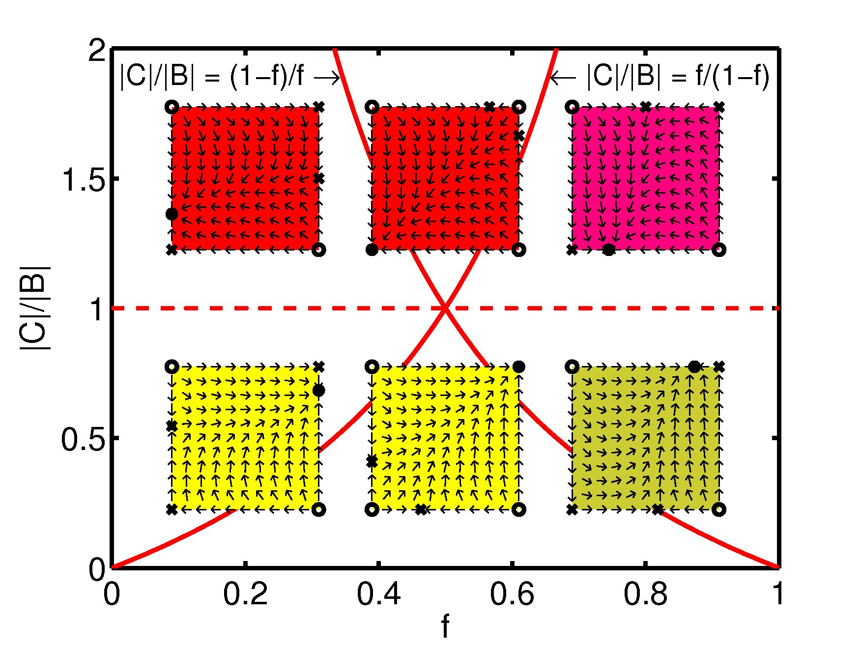
Figure 5: (Color Online) Illustration of the parameter-dependent types of outcomes in the multi-population snowdrift game, if $|C|/|B|$ and/or $f$ are varied and interaction between populations as well as self-interactions are considered. The representation and grey shades (colors) are the same as in Fig. 3.

While our previous analysis has been formal and abstract, we will now discuss our results in the context of social systems for the sake of illustration. Then, the entities are individuals, and the states represent behaviors. Without loss of generality, we assume $R>P$ (determining the numbering and meaning of behaviors) and $f\geq 1/2$ (determining the numbering of populations such that the power of population 1 is the same or greater than the one of population 2). Moreover, we will use the following terminology: If two interacting individuals show the same behavior, we will talk about “coordinated behavior”. The term “preferred behavior” is used for the preferred coordinated behavior, i.e. the behavior which gives the higher payoff, when the interaction partner shows the same behavior. This payoff is represented by $R$, while the non-preferred coordinated behavior results in the payoff $P$. Furthermore, if a focal individual chooses its preferred behavior and the interaction partner chooses a different behavior, the first one receives the payoff $S$ and the second one the payoff $T$. In the so-called prisoner’s dilemma, $R$ usually stands for “reward”, $T$ for “temptation”, $P$ for “punishment”, and $S$ for “sucker’s payoff”. The payoff-dependent parameter $C=R-T$ may be interpreted as gain of coordinating on one’s own preferred behavior (if greater than zero, otherwise as loss). Moreover, $B=S-P$ may be interpreted as gain when giving up coordinated, but non-preferred behavior.

The conflict of interest between two populations is reflected by the fact that “cooperative behavior” is a matter of perspective: A behavior that appears cooperative to a focal individual is cooperative from the viewpoint of its interaction partner only, if belonging to the same population, otherwise it is non-cooperative from the interaction partner’s viewpoint. In the model studied in this paper, population 1 prefers behavior 1, population 2 behavior 2. Moreover, behavior 1 corresponds to the cooperative behavior from the viewpoint of population 1, but to the non-preferred behavior of the interaction partner, i.e. it is non-cooperative from the point of view of population 2. Moreover, if two interacting individuals display the same behavior, their behavior is coordinated. Finally, we speak of a “behavioral norm” or of “normative behavior”, if all individuals (or the great majority) show the same (coordinated) behavior Epstein ; Levin ; Santos ; Fent , independently of their behavioral preferences and the (sub-)population they belong to. It should be stressed that this requires the individuals belonging to one of the populations to act against their own preferences. See Ref. JASSS for the related social science literature.

Within the context of the above definition, the four types of system dynamics distinguished above are related to four types of games discussed in the following:

1. For $T>R>P>S$ we have a multi-population prisoner’s dilemma (MPD), which corresponds to the case $B<0$ and $C<0$. According to the results in Sec. IV, this is characterized by a breakdown of cooperation. Accordingly, individuals in both populations will end up with their non-preferred behavior. This is even true, when the non-negative parameter $\nu$ in the generalized replicator equations (17) and (18) is different from 1.

2. In contrast, for $R>T>S>P$ we have a multi-population harmony game (MHG) with $B>0$ and $C>0$. In this case, all individuals end up with their preferred behaviors, but the behavior of both populations is not coordinated. Considering this coexistence of different behaviors, one could say that each population forms its own “subculture”.

3. For $R>T>P>S$, which implies $B<0$ and $C>0$, we are confronted with a multi-population stag-hunt game (MSH). For most initial conditions, the system ends up in the stationary states (1,0) or (0,1). In the first case, both populations coordinate themselves on the behavior preferred by population 1, while in the second case, they coordinate themselves on the behavior preferred by population 2. In both cases, all individuals end up with the same behavior. In other words, they establish a commonly shared behavior (a “social norm”). However, there are also conditions under which different behaviors coexist, namely if (1,1) or (0,0) is a stable stationary point (see yellow and red basins of attraction in Fig. 4 and in the MSH section of Fig. 3). Under such conditions, norms are not self-enforcing, as a commonly shared behavior may not establish. This relevant case can occur only, if both populations have interactions and self-interactions. It should also be noted that norms have a similar function in social systems that forces have in physics. They guide human interactions in subtle ways, creating a self-organization of social order. See Refs. JASSS ; HelEPJB for a more detailed discussion of these issues.

4. If $T>R>S>P$, corresponding to $B>0$ and $C<0$, we face a multi-population snowdrift game (MSD). In this case, it can happen that individuals in one of the populations (the stronger one) do not coordinate among each other. While some of their individuals show a cooperative behavior, the others are non-cooperative. We consider this fragmentation phenomenon as a simple description of social polarization or conflict.

Note that, in the multi-population snowdrift game with $B>0$ and $C<0$, the stationary point $(p_{5},0)$ exists for $f\geq|C|/(|B|+|C|)$, and the point $(p_{6},1)$ for $f\geq|B|/(|B|+|C|)$. If $f\geq 1/2$ and $(1-f)/f<|C|/|B|<f/(1-f)$, $(p_{5},0)$ is a stable fix point for $|B|<|C|$, while $(p_{6},1)$ is a stable fix point for $|B|>|C|$, which implies a discontinuous transition at the “critical” point $|B|=|C|$, when $|C|$ is continuously changed from values smaller than $|B|$ to values greater than $|B|$ or vice versa. This transition, where all individuals in the weaker population suddenly turn from cooperative behavior from the perspective of the stronger population to their own preferred behavior, may be considered to reflect a “revolution”. In the history of mankind, such revolutionary transitions have occured many times Weidlich .

It turns out to be insightful to determine the average fraction of cooperative individuals in both populations from the perspective of the stronger population 1. When $(p_{5},0)$ is the stable stationary point, it can be determined as the fraction of cooperative individuals in population 1 times the relative size $f$ of population 1, plus the fraction $1-q_{5}=1$ of non-cooperative individuals in population 2 (who are cooperative from the point of view of population 1), weighted by its relative size $(1-f)$:

$$p_{5}\!\cdot\!f+(1-q_{5})\!\cdot\!(1-f)\! = \!\frac{Bf+C(1-f)}{(B-C)f}\!\cdot\!f+1\!\cdot\!(1-f)$$ (38)

$$= \!\frac{B}{B-C}=\frac{|B|}{|B|+|C|}\,.$$

Similarly, if $(p_{6},1)$ is the stable stationary point, the fraction of cooperative individuals from the point of view of the stronger population 1 is given by

$$p_{6}\!\cdot\!f+(1-q_{6})\!\cdot\!(1-f)\! = \!\frac{B}{(B-C)f}\!\cdot\!f+0\!\cdot\!(1-f)$$ (39)

$$= \!\frac{B}{B-C}=\frac{|B|}{|B|+|C|}\,,$$

as for $q_{6}=1$, everybody in population 2 behaves non-cooperatively from the perspective of population 1. Surprisingly, the average fraction of cooperative individuals in both populations from the point of view of the stronger population corresponds exactly to the fraction $p_{0}=|B|/(|B|+|C|)$ of cooperative individuals expected in the one-population snowdrift game Preprint . However, this comes with an enormous deviation of the fraction $q$ of cooperative individuals in the weaker population 2 from the expected value $p_{0}$ (as we either have $q=0$ or $q=1$), and also with some degree of deviation of $p$ from $p_{0}$ in the stronger population 1. That is, although the stronger population in the multi-population snowdrift game causes an opposition of the weaker population and a polarization of society Note , the resulting distribution of behaviors in both populations finally reaches a result, which fits the expectation of the stronger population 1 (namely of having a fraction $p_{0}$ of cooperative individuals from the point of view of population 1). One could therefore say that the stronger population controls the behavior of the weaker population.

V Summary and Outlook

In this paper, we have used multi-population replicator equations to describe populations with conflicting interactions and different power. It turns out that the system’s behavior is much richer than in the one-population case or in the two-population case without self-interactions. Nevertheless, it is useful to distinguish four different types of games, characterized by a qualitatively different system dynamics: The harmony game, the prisoner’s dilemma, the stag-hunt game and the snowdrift game. When applied to social systems, the latter three describe social dilemma situations. However, in the presence of multiple populations, we may not only have the dilemma that people may choose not to cooperate. Their behaviors in different populations may also be uncoordinated. Accordingly, the establishment of cooperation is only one challenge in social systems, while the establishment of commonly shared behaviors (“social norms”) is another one. Note that the evolution of social norms is highly relevant for the evolution of language and culture Fortunato ; Skyrms ; Boyd . According to our model, it is expected to occur for multi-population stag hunt interactions. Interestingly, compared to the multi-population games without self-interactions, we have found several new subclasses, depending on the power $f$ of populations and the quotient $|C|/|B|$ of the payoff-dependent parameters $B$ and $C$. The same is true for multi-population snowdrift games.

Considering the simplicity of the model, the possible system behaviors are surprisingly rich. Besides the occurrence of phase transitions when $B$ and $C$ change their sign, we find additional transitions when $BC<0$ and the quotient $|C|/|B|$ crosses the values of 1, $f/(1-f)$, or $(1-f)/f$. We expect an even larger variety of system behaviors, if the model parameters are not chosen in a homogeneous way. For example, one could investigate cases in which both populations play different games. Our model can also be extended to study cases of migration and group selection. This will be demonstrated in forthcoming publications. It will also be interesting to compare the behavior of test persons in game-theoretical lab experiments Exp1 ; Exp2 with predictions of our model for interacting individuals with conflicting interests. Depending on the specification of the interaction payoffs, it should be possible to find the following types of system behaviors: (1) The breakdown of cooperation, (2) the coexistence of different behaviors (the establishment of “subcultures”), (3) the evolution of commonly shared behaviors (“norms”), and (4) the occurence of social polarization. In the latter case, one should also be able to find a “revolutionary transition” as $|B|/|C|$ crosses the value of 1. While there is empirical evidence that all these phenomena occur in real social systems, it will be interesting to test whether the above theory has also predictive power.

Author Contributions

D.H. developed the concept and model of this study, did the analytical calculations and wrote the manuscript. A.J. prepared the figures and supplementary videos, and he performed the underlying computer simulations.

Acknowledgements

The authors would like to thank for partial support by the ETH Competence Center “Coping with Crises in Complex Socio-Economic Systems” (CCSS) through ETH Research Grant CH1-01 08-2. They are grateful to Thomas Chadefaux, Ryan Murphy, Carlos Roca, Stefan Bechtold, Sergi Lozano, Heiko Rauhut, Wenjian Yu and further colleagues for valuable comments. D.H. thanks Thomas Voss for his insightful seminar on social norms.

References

- (1) The supplementary movies are accessible at http://www.soms.ethz.ch/research/twopopulationgames
- (2) J. von Neumann and O. Morgenstern, Theory of Games and Economic Behavior (Princeton University Press, Princeton, 1944).
- (3) J. Hofbauer K. Sigmund, Evolutionary Games and Population Dynamics (Cambridge University, Cambridge, 1998).
- (4) J. W. Weibull, Evolutionary Game Theory (MIT Press, Cambridge, MA, 1996).
- (5) R. Cressman, Evolutionary Dynamics and Extensive Form Games (MIT Press, Cambridge, MA, 2003).
- (6) M. Nowak, Evolutionary Dynamics. Exploring the Equations of Life (Belknap Press, Cambride, MA, 2006).
- (7) D. Helbing, Interrelations between stochastic equations for systems with pair interactions. Physica A 181, 29–52 (1992); D. Helbing, Boltzmann-like and Boltzmann-Fokker-Planck equations as a foundation of behavioral models. Physica A 196, 546–573 (1993).
- (8) D. Challet, M. Marsili, and R. Zecchina, Statistical mechanics of systems with heterogeneous agents: Minority games. Physical Review Letters 84 1824–1827 (2000).
- (9) C. P. Roca, J. A. Cuesta, and A. Sánchez, Time scales in evolutionary dynamics Phys. Rev. Lett. 97 158701 (2006).
- (10) J. C. Claussen and A. Traulsen, Cyclic dominance and biodiversity in well-mixed populations. Phys. Rev. Lett. 100, 058104 (2008).
- (11) A. Traulsen, J. C. Claussen, and C. Hauert, Coevolutionary dynamics: From finite to infinite populations. Phys. Rev. Lett. 95 238701 (2005).
- (12) R. Axelrod, The Evolution of Cooperation (Basic Books, New York, 1984).
- (13) H. Gintis, Game Theory Evolving (Princeton University, Princeton, NJ, 2000).
- (14) B. Skyrms, The Stag Hunt and the Evolution of Social Structure (Cambridge University, Cambridge, 2003).
- (15) R. Boyd, P. J. Richerson, The Origin and Evolution of Cultures (Oxford University, Oxford, 2005).
- (16) H. Gintis, The Bounds of Reason. Game Theory and the Unification of the Behavioral Sciences (Princeton University Press, Princeton, 2009).
- (17) K. Binmore, Playing for Real (Oxford University Press, Oxford, 2007).
- (18) J. Henrich, R. Boyd, S. Bowles, C. Camerer, E. Fehr, H. Gintis (eds.) Foundations of Human Sociality: Economic Experiments and Ethnographic Evidence from Fifteen Small-Scale Societies (Oxford University Press, Oxford, 2004).
- (19) A. Traulsen, C. Hauert, H. De Silva, M. A. Nowak, K. Sigmund, Exploration dynamics in evolutionary games. PNAS 106(3), 709–712 (2009).
- (20) D. Helbing and T. Vicsek, Optimal self-organization, New Journal of Physics 1, 13 (1999).
- (21) D. Helbing and T. Platkowski, Drift- or fluctuation-induced ordering and self-organization in driven many-particle systems Europhys. Lett. 60 227–233 (2002).
- (22) V. M. de Oliveira and J. F. Fontanari, Random replicators with high-order interactions. Phys. Rev. Lett. 85, 4984–4987 (2000).
- (23) D. Helbing and S. Lozano, Routes to cooperation and adaptive group pressure in the prisoner’s dilemma, submitted (2009).
- (24) D. Helbing, A mathematical model for behavioral changes by pair interactions, in G. Haag, U. Mueller, K. G. Troitzsch (Eds.) Economic Evolution and Demographic Change (Springer, Berlin, 1992), pp. 330–348; D. Helbing, A stochastic behavioral model and a ‘microscopic’ foundation of evolutionary game theory. Theory and Decision 40, 149–179 (1996).
- (25) H. P. Young, The evolution of conventions, Econometrica 61, 57–84 (1993).
- (26) F. Schweitzer, L. Schimansky-Geier, W. Ebeling, and H. Ulbricht, A stochastic approach to nucleation in finite systems: Theory and computer simulations. Physica A 150, 261–279 (1988).
- (27) F. Schweitzer and L. Schimansky-Geier, Clustering of active walkers in a two-component system. Physica A 206, 359–379 (1994).
- (28) M. Eigen and P. Schuster, The Hypercycle (Springer, Berlin, 1979).
- (29) R. A. Fisher, The Genetical Theory of Natural Selection (Oxford University Press, Oxford, 1930).
- (30) W. Ebeling, A. Engel, and R. Feistel, Physik der Evolutionsprozesse [Physics of Evolutionary Processes, in German] (Akademie Verlag, Berlin, 1990).
- (31) J. Hofbauer, On the occurrence of limit cycles in the Volterra-Lotka equation. Nonlinear Analysis, Theory, Methods & Applications 5, 1003–1007 (1981).
- (32) N. S. Goel, S. C. Maitra, and E. W. Montroll, On the Volterra and other nonlinear models of interacting populations. Rev. Mod. Phys. 43, 231–276 (1971).
- (33) R. M. May, Stability and Complexity in Model Ecosystems (Princeton University Press, Princeton, NJ, 2001).
- (34) V. M. de Oliveira and J. F. Fontanari, Complementarity and diversity in a soluble model ecosystem, Phys. Rev. Lett. 89, 148101 (2002).
- (35) J. Y. Wakano, M. A. Nowak, and C. Hauert, Spatial dynamics of ecological public goods. PNAS 106, 7910–7914 (2009).
- (36) M. A. Nowak and R. M. May, Evolutionary games and spatial chaos. Nature 359, 826–829 (1992).
- (37) G. Szabó and C. Hauert, Phase transitions and volunteering in spatial public goods games. Phys. Rev. Lett. 89, 118101 (2002).
- (38) C. P. Roca, J. A. Cuesta, and A. Sánchez, Evolutionary game theory: Temporal and spatial effects beyond replicator dynamics. Physics of Life Reviews, in press (2009).
- (39) G. Szabó and G. Fath, Evolutionary games on graphs. Phys. Rep. 446, 97–216 (2007).
- (40) G. Abramson and M. Kuperman, Social games in a social network. Phys. Rev. E 63, 030901 (2001).
- (41) J. M. Pacheco, A. Traulsen and M. A. Nowak, Co-evolution of strategy and structure in complex networks with dynamical linking Phys. Rev. Lett. 97 258103 (2006).
- (42) L.-X. Zhong 1 - D.-F. Zheng 1 - B. Zheng 1 - C. Xu 2 - P. M. Hui 2 Networking effects on cooperation in evolutionary snowdrift game, Europhys. Lett. 76, p. 724 (2006).
- (43) F. C. Santos, J. M. Pacheco, and T. Leanerts, Evolutionary dynamics of social dilemmas in structured heterogeneous populations. PNAS 103(9), 3490–3494 (2006).
- (44) H. Ohtsuki, M. A. Nowak, and J. M. Pacheco, Breaking the symmetry between interaction and replacement in evolutionary dynamics on graphs. Phys. Rev. Lett. 98 108106 (2007).
- (45) S. Lozano, A. Arenas, and A. Sanchez, Mesoscopic structure conditions the emergence of cooperation in social networks, PLoS ONE 3, 4 (2008).
- (46) A. Szolnoki, M. Perc, and Z. Danku, Making new connections towards cooperation in the prisoner’s dilemma game, Europhys. Lett. 84, 50007 (2008).
- (47) T. Reichenbach, M. Mobilia, and E. Frey, Mobility promotes and jeopardizes biodiversity in rock-paper-scissors games. Nature 448, 1046–1049 (2007).
- (48) D. Helbing and T. Platkowski, Self-organization in space and induced by fluctuations. International Journal of Chaos Theory and Applications 5(4), 47–62 (2000).
- (49) D. Helbing and W. Yu (2008) Migration as a mechanism to promote cooperation. Advances in Complex Systems 11(4) 641 - 652.
- (50) D. Helbing (2009) Pattern formation, social forces, and diffusion instability in games with success-driven motion European Physical Journal B 67, 345–356.
- (51) D. Helbing and W. Yu (2009) The outbreak of cooperation among success-driven individuals under noisy conditions. Proceedings of the National Academy of Sciences USA (PNAS) 106(8), 3680-3685.
- (52) M. Perc, Chaos promotes cooperation in the spatial prisoner’s dilemma game, Europhys. Lett. 75, 841 (2006).
- (53) W. Yu and D. Helbing, Game theoretical interactions of moving agents, e-print http://arxiv.org/abs/0903.0987
- (54) C. P. Roca, J. A. Cuesta, and A. Sánchez, Imperfect imitation can enhance cooperation. Europhys. Lett. 87, 48005 (2009).
- (55) M. A. Nowak, Five rules for the evolution of cooperation. Science 314, 1560–1563 (2006).
- (56) P. Schuster, K. Sigmund, J. Hofbauer, R. Gottlieb, P. Merz, Selfregulation of behaviour in animal societies. III. Games between two populations with selfinteraction. Biological Cybernetics 40, 17–25 (1981).
- (57) K. Argasinski, Dynamic multipopulation and density dependent evolutionary games related to replicator dynamics. A metasimplex concept. Mathematical Biosciences 202, 88–114 (2006).
- (58) T. Kanazawa, Multi-population replicator dynamics with changes of interpretations and strategies. IEICE Trans. Fundamentals E 89–A(10), 2717–2723 (2006).
- (59) K. H. Schlag, Why imitate, and if so, how? A boundedly rational approach to multi-armed bandits. Journal of Economic Theory 78(1), 130–156 (1998).
- (60) D. Helbing and A. Johansson, Cooperation, norms, and revolutions: A unified game-theoretical approach. Submitted (2009).
- (61) J. M. Epstein, Learning to be thoughtless: Social norms and individual computation. Computational Economics 18, 9–24 (2001).
- (62) P. R. Ehrlich, S. A. Levin, The evolution of norms. PLoS Biology 3(6), 0943–0948 (2005).
- (63) F. A. C. C. Chalub, F. C. Santos, J. M. Pacheco, The evolution of norms. Journal of Theoretical Biology 241, 233–240 (2006).
- (64) T. Fent, P. Groeber, and F. Schweitzer, Coexistence of social norms based on in- and out-group interactions. Advances of Complex Systems 10(2), 271–286 (2007).
- (65) W. Weidlich, H. Huebner, Dynamics of political opinion formation including catastrophe theory. Journal of Economic Behavior & Organization 67, 1–26 (2008).
- (66) Here, we understand “polarization” in the sense that a population fragments into parts with different behaviors.
- (67) C. Castellano, S. Fortunato, and V. Loreto, Statistical physics of social dynamics. Rev. Mod. Phys. 81, 591–646 (2009).
- (68) D. Helbing, M. Schönhof, and D. Kern, Volatile decision dynamics: Experiments, stochastic description, intermittency control, and traffic optimization. New J. Phys. 4, 33 (2002).
- (69) D. Helbing, M. Schönhof, H.-U. Stark, and J. A. Holyst, How individuals learn to take turns: Emergence of alternating cooperation in a congestion game and the prisoner’s dilemma. Advances in Complex Systems 8, 87–116 (2005).