RR Lyrae variables in M32 and the disk of M31

Abstract

We observed two fields near M32 with the Advanced Camera for Surveys/High Resolution Channel (ACS/HRC) on board the Hubble Space Telescope (HST). The main field, F1, is 1$\farcm$8 from the center of M32; the second field, F2, constrains the M31 background, and is 5$\farcm$4 distant. Each field was observed for 16-orbits in each of the $F435W$ (narrow $B$) and $F555W$ (narrow $V$) filters. The duration of the observations allowed RR Lyrae stars and other short-period variables to be detected. A population of RR Lyrae stars determined to belong to M32 would prove the existence of an ancient population in that galaxy, a subject of some debate.

We detected 17 RR Lyrae variables in F1 and 14 in F2. A $1\sigma$ upper limit of 6 RR Lyrae variables belonging to M32 is inferred from these two fields alone. Use of our two ACS/WFC parallel fields provides better constraints on the M31 background, however, and implies that $7_{-3}^{+4}$ (68 % confidence interval) RR Lyrae variables in F1 belong to M32. We have therefore found evidence for an ancient population in M32. It seems to be nearly indistinguishable from the ancient population of M31. The RR Lyrae stars in the F1 and F2 fields have indistinguishable mean $V$-band magnitudes, mean periods, distributions in the Bailey diagram and ratios of RRc to RR_total types. However, the color distributions in the two fields are different, with a population of red RRab variables in F1 not seen in F2. We suggest that these might be identified with the detected M32 RR Lyrae population, but the small number of stars rules out a definitive claim.

1. Introduction

Messier 32 (M32) is the only elliptical galaxy close enough to possibly allow direct observation of its stars down to the main-sequence turn-off (MSTO). It is a vital laboratory for deciphering the stellar populations of all other elliptical galaxies, which can only be studied by the spectra of their integrated light, given their greater distances. Major questions about M32’s star formation history remain unanswered. M32 appears to have had one or more relatively recent episodes of star formation (within the last 3 Gyr: e.g., O’Connell, 1980; Rose, 1985, 1994; González, 1993; Trager et al., 2000; Coelho et al., 2009), which also appears to be true for many elliptical galaxies (e.g., González, 1993; Trager et al., 2000; Thomas et al., 2005). These conclusions rest on painstaking and controversial spectral analysis of their integrated light. In contrast, the most direct information about a stellar population comes from applying stellar evolution theory to color–magnitude diagrams (CMDs). Little however is known about M32’s ancient population (see, e.g., Brown et al., 2000; Coelho et al., 2009).

With our Advanced Camera for Surveys/High Resolution Channel (ACS/HRC) data (Cycle 14, Program GO-10572, PI: T. Lauer) we have obtained the deepest CMD of M32 to date. A comprehensive analysis of this CMD is discussed in a companion paper Monachesi et al. (2009, hereafter M09) and we refer to it for further details. However here we want to stress that, due to the severe crowding in our fields, even with the high spatial resolution of HRC it is not possible to reach the MSTO with sufficient precision to claim the presence of a very old population.

RR Lyrae variables are low-mass stars burning He in their cores. They are excellent tracers of ancient stellar populations, completely independent of the MSTO, and knowledge of their properties provides important information on their parent stellar populations. Because they are located on the horizontal branch (HB) in a CMD, they are at least 3 magnitudes brighter than MSTO dwarfs and therefore detectable to relatively large distances. RR Lyrae are also very easy to characterize, with ab-type RR Lyrae (RRab) pulsating in the fundamental mode, rising rapidly to maximum light and slowly declining to minimum light, and c-type RR Lyrae (RRc) pulsating in the first harmonic mode, with their luminosities varying roughly sinusoidally. Most importantly for our purpose, the mere presence of RR Lyrae stars among a population of stars suggests an ancient origin, as ages older than $\sim 10$ Gyr are required to produce RR Lyrae variables. Thus the detection of RR Lyrae stars in M32 is presently the only way to confirm the existence of an ancient stellar population in this galaxy.

Alonso-García et al. (2004) were the first to attempt to directly detect RR Lyrae stars in fields near M32. They imaged a field $\sim 3\farcm 5$ with WFPC2 to the east of M32 and compared it with a control field well away from M32 that should sample the M31 field stars. They identified $12\pm 8$ variable stars claimed to be RR Lyrae stars belonging to M32 and therefore suggested that M32 possesses a population that is older than $\sim 10$ Gyr. They were however unable to classify these RR Lyrae variables and could not derive periods and amplitudes for them.

Very recently, Sarajedini et al. (2009, hereafter S09) used ACS/WFC parallel imaging from our present data set to find RR Lyrae variables in two fields close to M32. They found 681 RR Lyrae variables, with excellent photometric and temporal completeness (Sec. 4). These RR Lyrae stars were roughly equally distributed between the two fields, with the same mean average magnitudes, metallicities, and Oosterhoff types in each field. It was therefore impossible for them to separate the variables into M31 and M32 populations. It is still therefore an open question as to the precise nature or even presence of RR Lyrae variables in M32.

In this paper, we present newly-detected RR Lyrae variables observed with ACS/HRC and also a detailed analysis of the fields near M32 where RR Lyrae stars have been found with HST. The paper is organized as follows. In Section 2 we describe our observations and the data reduction we performed. We move on to describe the technique used to identify and characterize the RR Lyrae variable stars in Section 3, where we present their periods and light curves. In Section 4 we show that we have clearly detected RR Lyrae variables in M32, as long as we include the results from our ACS/WFC parallel fields. In Section 5 we discuss the properties of the RR Lyrae stars, such as the location of their instability strip, reddenings, mean periods and Oosterhoff types, as well as pulsational relations such as period–metallicity–amplitude. In this section we also derive estimates of the distance moduli to and metallicities of our fields. We summarize our findings and present our final conclusions in Section 6.

2. Observations and Data reduction

Table 1Log of observations

Field	$\alpha_{J2000.0}$	$\delta_{J2000.0}$	Filter	Exposure time	Date
F1	00 42 47.63	+40 50 27.4	$F435W$	16$\times$1279 + 16$\times$1320	20–22 Sep 2005
F1	00 42 47.63	+40 50 27.4	$F555W$	16$\times$1279 + 16$\times$1320	22–24 Sep 2005
F2	00 43 07.89	+40 54 14.5	$F435W$	16$\times$1279 + 16$\times$1320	6–8 Feb 2006
F2	00 43 07.89	+40 54 14.5	$F555W$	16$\times$1279 + 16$\times$1320	9–12 Feb 2006

2.1. Field Selection, Observational Strategy and Data Reduction

We obtained deep $B$ and $V$-band imaging of two fields near M32 using the ACS/HRC instrument on board HST during Cycle 14 (Program GO-10572, PI: Lauer). The primary goal of this program was to resolve the M32 MSTO. The ACS $F435W$ ($B$) and $F555W$ ($V$) filters were selected to optimize detection of MSTO stars over the redder and more luminous stars of the giant branch. M32 is very compact and is projected against the M31 disk. Thus the major challenge was to select a field that represented the best compromise between the extreme crowding in M32, which would drive the field to be placed as far away from the center of the galaxy as possible, versus maximizing the contrast of M32 against the M31 background populations, which would push the field back towards the central, bright portions of M32. Following these constraints, the M32 HRC field (designated F1) was centered on a location $110\arcsec$ south (the anti-M31 direction) of the M32 nucleus, roughly on the major axis of the galaxy. The $V$-band surface brightness of M32 near the center of the field is $\mu_{V}\approx 21.9$ (Kormendy et al., 2009). M32 quickly becomes too crowded to resolve faint stars at radii closer to the center, while the galaxy rapidly falls below the M31 background at larger radii.

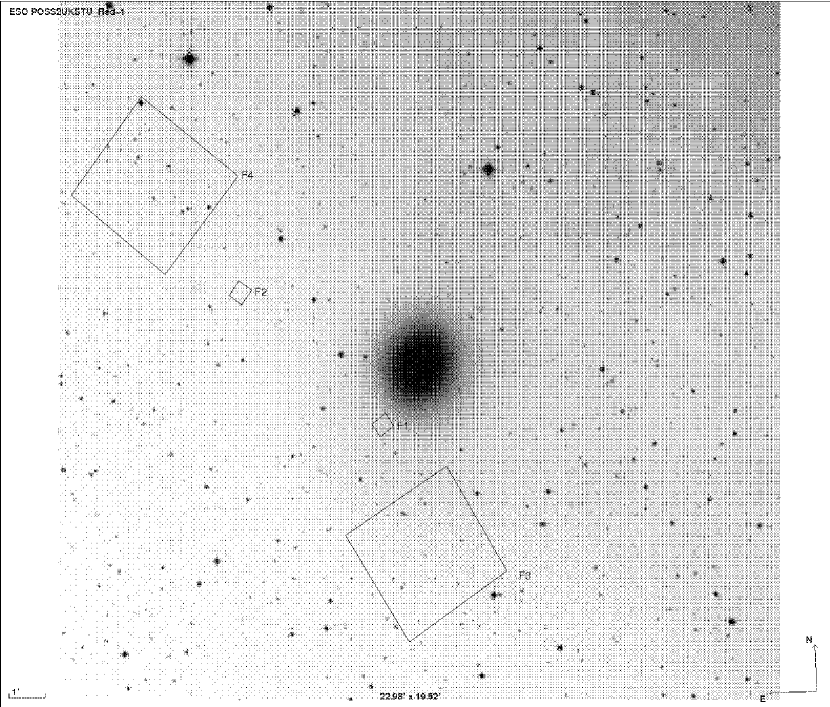
Figure 1.— Location of our pointings near M32 observed with ACS/HRC on board HST (small squares). Fields F1 and F2 are at distances of 1$\farcm$8 and 5$\farcm$4 from the center of M32, respectively, and each of them covers a region of 0.25 arcmin² on the sky. Parallel fields, taken with ACS/WFC, F3 and F4 are at distances of 5$\farcm$3 and 9$\farcm$2 from the center of M32, respectively, covering a region of 9 arcmin² on the sky.

Even at the location of F1, M31 contributes $\sim 1/3$ of the total light, thus it was critical to obtain a background field, F2, at the same isophotal level in M31 ($\mu_{V}\sim 22.7$) to allow for the strong M31 contamination to be subtracted from the analysis of the M32 stellar population. F2 was located $327\arcsec$ from the M32 nucleus at position angle $65^{\circ}.$ At this angular distance M32 has an ellipticity $\epsilon\approx 0.25$ (Choi et al., 2002), and F2 is nearly aligned with the M32 minor-axis. Thus the implied semi-major axis of the M32 isophote that passes though F2 is $435\arcsec$, significantly larger than the nominal angular separation. The estimated M32 surface brightness at F2 is $\mu_{V}\approx 27.5,$ based on a modest extrapolation of the $B$-band surface photometry of Choi et al. (2002) and an assumed color of $B-V\approx 0.9$. The contribution of M32 to F2 thus falls by a factor of $\sim 180$ relative to its surface brightness at F1. While one might have been tempted to move F2 even further away from F1, it clearly serves as an adequate background at the location selected, while uncertainties in the M31 background would increase at larger angular offsets. The locations of both the F1 and F2 fields are shown in Figure 1.

Detection of the MSTO required deep exposures at F1. Accurate treatment of the background required equally deep exposures to be obtained in F2. A summary of the observations is shown in Table 1; briefly, each field was observed for 16 orbits in each of the $F435W$ and $F555W$ filters for a total program of 64 orbits. While the detection of RR Lyrae variables was not the primary goal of the program, execution of each filter/field combination in a contiguous time span of 2–3 days was clearly well-suited to detect RR Lyrae variables, which have periods ranging from 0.2–1 d.

At $B$ and $V$, the HRC undersamples the PSF, despite its exceptionally fine pixel scale. All of the images were obtained in a $0.5\times 0.5$ sub-pixel square dither pattern to obtain Nyquist sampling in the complete data set. In detail, the sub-pixel dither pattern was executed across each pair of orbits, with each orbit split into two sub-exposures. The telescope was then offset by $0\farcs 125$ steps between the orbit pairs in a “square-spiral” dither pattern to minimize the effects of “hot pixels,” bad columns, and any other fixed-defects in the CCD, on the photometry at any location. The data for each filter/field combination thus comprises 8 slightly different pointings, with Nyquist-sampling obtained at each location. In practice, the dithers were extremely accurate, and Nyquist images could readily be constructed using the algorithm of Lauer (1999).

Our optimal average photometry has been obtained by using these very deep, super-resolved images. We have performed photometry by using both the DAOPHOT II/ALLSTAR packages (Stetson, 1987, 1994) and by first deconvolving those combined images with a reliable PSF and then performing aperture photometry on the deconvolved images. Both methods returned comparable results and allow us to present the deepest CMD of M32 obtained so far. This result is analyzed in M09 and will not be discussed further here. However, in what follows we will use these CMDs to show the location of RR Lyrae stars.

In addition to the HRC images, parallel observations were obtained with the ACS/WFC channel using the $F606W$ filter (broad $V$). These fields, designated F3 and F4, are also shown in Figure 1. Notably, the telescope rolled by roughly $180^{\circ}$ between the execution of the F1 and F2 observations, thus F3, the parallel field associated with F1, and F4, the mate to F2, bracket the F1 and F2 fields in angle. By happenstance, the F3 and F4 fields also nearly fall on the same M31 isophote that encompasses the F1 and F2 fields, thus the M31 background should be roughly similar in all four fields. It is also notable that F3 is positioned slightly closer to the M32 nucleus than F2 ($317\arcsec$ versus $327\arcsec$), but because it also falls along the M32 major rather than minor axis, its associated M32 surface brightness is $\mu_{V}\sim 25$, or a factor of $\sim 10\times$ more than the M32 contribution to F2. Furthermore we note that the parallel observations were exposed only at the same time as the $F555W$ exposures in F1 and F2 and therefore cover only half of the total time window of the primary exposures (we return to this point in Sec. 4 below).

The parallel images have already been analyzed by S09. They find 681 RR Lyrae variables stars, of which 324 are located in the field closest to M32. Because only one filter was available for the parallel observations, S09 did not have all the information needed to properly disentangle the populations that belong to M31 and/or M32. In fact, their detected RR Lyrae stars show the same mean average magnitude, metallicity and Oosterhoff type, as we discuss in Section 5. With our primary observations we can attempt to disentangle the two populations by using all the quantities characterizing the class of RR Lyrae variables, such as mean weighted magnitudes and colors in the Johnson-Cousins system, periods, and amplitudes.

2.2. Photometry of the RR Lyrae Variables

The study of the presence of RR Lyrae stars is based on a detailed analysis of the time series of our fields. We analyzed each single epoch image (32 per field and per filter) and not the combination of all the images described above. Because of the intrinsic brightness of the RR Lyrae ($V\sim 25$ mag), we decided to perform PSF-fitting photometry over all the fully calibrated data products (FLT) images using the DOLPHOT package, a version of HSTphot (Dolphin, 2000) modified for ACS images. Our choice has been justified by the short time consumed to obtain high quality photometry at the RR Lyrae magnitude level for our data set. Following the DOLPHOT User’s Guide, we have performed the pre-processing steps mask and calcsky routines before running DOLPHOT. This package performs photometry simultaneously over all 64 images of each field, returning a catalog of more than 20000 stars per field already corrected for charge transport efficiency (CTE) and aperture correction, following the suggestions by Sirianni et al. (2005). We use this photometry to perform the analysis of variable stars.

2.2.1 Photometric Completeness at the Horizontal Branch

The 50% completeness levels of fields F1 and F2 are at least 2 mag deeper than the horizontal branch, as shown by the artificial star tests (ASTs) in M09. The ASTs show that the completeness at the red clump (i.e., the red horizontal branch) is 100%. The ASTs in M09 do not properly populate the blue horizontal branch, as there are very few stars in this region of the CMD, so we assume that the completeness at the position of the blue horizontal branch is the same as at the red clump.

3. Searching for variable stars and their periods

To identify variable sources in both fields, we used a code written by one of us (AS) in the Interactive Data Language (IDL) whose principles, based on the algorithm of Lafler & Kinman (1965), are discussed in Saha & Hoessel (1990). This code was applied to the results from DOLPHOT PSF-fitting photometry described in the previous section. Its output gives us not only a list of candidate variable stars but also a good initial estimate of their periods. The method assumes that realistic error estimates for each object at each epoch are available from the photometry, which are first used to estimate a chi-square based probability that any given object is a variable. A list of candidates is then chosen, and each candidate is tested for periodicity and plausible light curves. The graphical interface of this program clearly shows possible aliases and allows the user to examine the light curves implied for each such alias. The final decision making is done by the user. A refinement of the period for all the candidate variables has been performed by using two other independent codes. We used the Period Dispersion Minimization (PDM) algorithm in the IRAF environment to confirm the found periodicity (Stellingwerf, 1978). Further refinement was then obtained by using GRATIS (GRaphical Analyzer of TIme Series, developed by P. Montegriffo at the Bologna Observatory; see Clementini et al. 2000 and references therein for details), which permits us to fit Fourier series to the magnitudes in each passband as a function of their phase.

Table 2F1 RR Lyrae properties

Star id	RA	DEC	Period	H	Epoch	$F435W$	$F555W$	$\langle V\rangle$	$\langle B\rangle-\langle V\rangle$	$A_{B}$	$A_{V}$	res$B$	res$V$	type
	J2000	J2000	(days)		(JD)	mag	mag	mag	mag	mag	mag	mag	mag
1	00:42:48.435	+40:50:32.11	0.255	1	2453634.900	25.56	25.39	25.44	0.19	0.64	0.59	0.11	0.10	RRc
2	00:42:46.509	+40:50:30.19	0.285	1	2453633.060	25.68	25.45	25.50	0.24	0.77	0.56	0.12	0.11	RRc
3	00:42:46.563	+40:50:23.03	0.311	1	2453632.810	25.42	25.22	25.30	0.19	0.61	0.58	0.09	0.11	RRc
4	00:42:48.237	+40:50:12.85	0.317	1	2453632.900	25.59	25.43	25.47	0.20	0.61	0.42	0.12	0.10	RRc
5	00:42:48.384	+40:50:30.61	0.475	2	2453636.290	25.52	25.29	25.34	0.25	0.99	0.85	0.10	0.11	RRab
6	00:42:47.349	+40:50:41.91	0.486	3	2453634.450	25.93	25.56	25.60	0.41	1.09	0.82	0.15	0.15	RRab
7	00:42:48.074	+40:50:30.17	0.519	4	2453634.415	25.34	25.04	25.09	0.31	1.01	0.75	0.08	0.06	RRab
8	00:42:47.552	+40:50:30.41	0.521	3	2453634.560	25.68	25.41	25.46	0.28	0.93	0.76	0.09	0.10	RRab
9	00:42:47.087	+40:50:43.08	0.523	3	2453635.650	25.61	25.25	25.29	0.40	1.09	1.06	0.12	0.13	RRab
10	00:42:47.034	+40:50:28.29	0.546	3	2453632.216	25.93	25.51	25.55	0.45	1.41	1.03	0.18	0.16	RRab
11	00:42:47.462	+40:50:42.81	0.564	2	2453635.490	25.51	25.19	25.21	0.36	0.74	0.68	0.15	0.09	RRab
12	00:42:48.737	+40:50:32.31	0.621	2	2453632.600	25.43	25.19	25.18	0.30	1.25	0.89	0.17	0.15	RRab
13	00:42:47.014	+40:50:36.27	0.625	2	2453637.280	25.57	25.28	25.29	0.35	0.88	0.68	0.09	0.08	RRab
14	00:42:46.411	+40:50:29.96	0.626	3	2453632.500	25.53	25.15	25.19	0.43	1.09	0.81	0.09	0.09	RRab
15	00:42:47.554	+40:50:16.48	0.645	3	2453634.680	25.83	25.47	25.50	0.40	0.74	0.39	0.10	0.07	RRab
16	00:42:46.075	+40:50:25.38	0.728	2	2453637.320	25.74	25.22	25.25	0.58	0.39	0.38	0.12	0.08	RRab
17	00:42:46.638	+40:50:25.24	0.851	2	2453637.693	25.60	25.15	25.17	0.49	0.65	0.45	0.10	0.08	RRab

Table 3F2 RR Lyrae properties

Star id	RA	DEC	Period	H	Epoch	$F435W$	$F555W$	$\langle V\rangle$	$\langle B\rangle-\langle V\rangle$	$A_{B}$	$A_{V}$	res$B$	res$V$	type
	J2000	J2000	(days)		(JD)	mag	mag	mag	mag	mag	mag	mag	mag
1	00:43:07.766	+40:54:15.31	0.267	2	2453772.400	25.46	25.32	25.38	0.20	0.66	0.59	0.09	0.09	RRc
2	00:43:07.704	+40:54:23.18	0.287	2	2453774.700	25.47	25.36	25.41	0.18	0.70	0.55	0.10	0.07	RRc
3	00:43:08.518	+40:54:08.86	0.320	2	2453774.125	25.51	25.26	25.31	0.33	0.46	0.43	0.08	0.09	RRc
4	00:43:07.734	+40:54:27.17	0.326	2	2453774.310	25.51	25.36	25.41	0.24	0.57	0.47	0.10	0.09	RRc
5	00:43:07.874	+40:54:31.99	0.350	1	2453777.220	25.45	25.25	25.30	0.28	0.60	0.42	0.11	0.09	RRc
6	00:43:08.300	+40:54:21.88	0.383	2	2453771.830	25.25	25.08	25.14	0.23	0.63	0.49	0.07	0.07	RRc
7	00:43:07.671	+40:54:01.99	0.482	3	2453778.050	25.53	25.33	25.39	0.28	1.37	1.08	0.15	0.12	RRab
8	00:43:08.339	+40:54:23.36	0.502	3	2453774.324	25.64	25.32	25.37	0.39	1.19	1.05	0.12	0.14	RRab
9	00:43:07.594	+40:54:21.32	0.528	3	2453773.198	25.53	25.27	25.30	0.35	1.27	1.02	0.11	0.11	RRab
10	00:43:07.424	+40:54:26.69	0.528	3	2453774.846	25.40	25.17	25.23	0.29	1.26	0.89	0.13	0.12	RRab
11	00:43:07.727	+40:54:13.25	0.571	2	2453775.520	25.52	25.28	25.35	0.28	1.06	0.99	0.15	0.14	RRab
12	00:43:08.107	+40:54:21.00	0.588	3	2453775.045	25.64	25.36	25.41	0.35	0.94	0.81	0.10	0.10	RRab
13	00:43:07.977	+40:54:21.33	0.697	2	2453778.053	25.40	25.12	25.19	0.33	0.70	0.58	0.09	0.06	RRab
14	00:43:07.798	+40:54:14.39	0.790	2	2453778.450	25.28	24.95	25.00	0.40	0.63	0.56	0.07	0.08	RRab

Table 4Time-series magnitudes for RR Lyrae variables

Julian date	F435W	$B$	Julian date	F555W	$V$
$-$2400000	mag	mag	$-$2400000	mag	mag
F1 variable 1
53633.616	25.39$\pm$0.07	25.44	53635.480	25.42$\pm$0.07	25.48
53633.631	25.22$\pm$0.06	25.28	53635.496	25.60$\pm$0.08	25.66
53633.681	25.36$\pm$0.07	25.42	53635.545	25.72$\pm$0.08	25.78
53633.697	25.69$\pm$0.09	25.74	53635.560	25.62$\pm$0.08	25.67
53633.748	25.96$\pm$0.10	26.01	53635.612	25.44$\pm$0.06	25.50
53633.764	25.89$\pm$0.10	25.93	53635.628	25.24$\pm$0.06	25.29
53633.814	25.86$\pm$0.10	25.90	53635.678	25.25$\pm$0.06	25.31
53633.830	25.50$\pm$0.07	25.55	53635.694	25.24$\pm$0.06	25.30
53634.415	25.39$\pm$0.08	25.44	53636.213	25.17$\pm$0.06	25.22
53634.430	25.37$\pm$0.08	25.42	53636.228	25.38$\pm$0.07	25.44

Note. — The errors on HST VEGAMAG are the photometrical ones. The calibration onto the Johnson-Cousins $B$- and $V$-bands as well as their errors have been discussed in the text. This is a sample table showing the format of the Table; the complete table can be found in the online version of the journal.

The magnitudes returned by DOLPHOT have already been calibrated onto the HST VEGAMAG photometric system, but for the following analysis we need to transform them onto the Johnson-Cousins (JC) system. We need therefore to take into account the color variations in the periodic cycles of the variable stars. We thus associate each phased epoch in the $F435W$ filter with the corresponding best-fitting $F555W$ model provided by GRATIS at that epoch, and vice versa. Finally, we apply the Sirianni et al. (2005) transformations from $F435W$ and $F555W$ to $B$ and $V$ for ACS/HRC, and we re-analyze the new JC time series with GRATIS to improve the light curve models as well as the previously-constrained periods. The order of the Fourier series used to obtain the best fit and the epoch corresponding to maximum of the light curve at phase $\phi=1$ are given in columns 5 and 6 in Tables 2 and 3. This procedure allows us to derive well-sampled and consistent light curves in both filters. Proper periods, mean magnitudes weighted on the proper light curve in both HST VEGAMAG and JC photometric systems, colors, and amplitudes are given in Tables 2 and 3 for a total number of 31 bona fide RR Lyrae stars: 17 in F1 and 14 in F2. The time series photometry is given in Table 4.

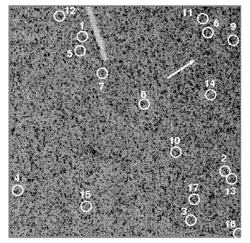
Figure 2.— Finding chart for RR Lyrae variables found in field F1. Numbers correspond to variables listed in Table 2. The FoV size is 0.25 arcmin², as listed in column 9 of Table 5. We note that the RR Lyrae stars in F1 are slightly clustered along the edge closest to the center of M32 where the total stellar density is increasing; we return to this point in Section 5.1. The arrow points towards the center of M32.

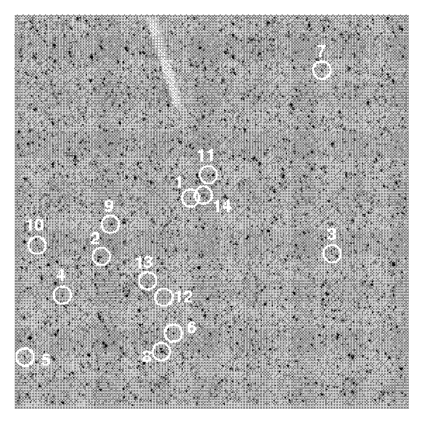
Figure 3.— Finding charts for RR Lyrae variables found in field F2. Numbers correspond to variables listed in Table 3. The FoV size is 0.25 arcmin², as listed in column 9 of Table 5. The adopted intensity scale is the same as in Fig. 2 for a fair comparison.

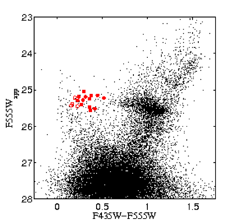
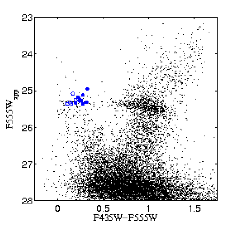
Figure 4.— The ($F435W-F555W$, $F555W$) CMDs calibrated onto the HST VEGAMAG photometric system for fields F1 (left) and F2 (right). We show the location of the detected RR Lyrae variable stars. First-overtone (FO) and fundamental-mode (FU) pulsators are shown with empty and filled circles respectively. These CMDs are presented and discussed in M09.

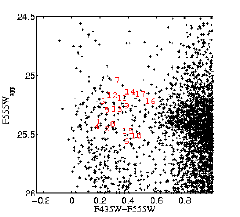
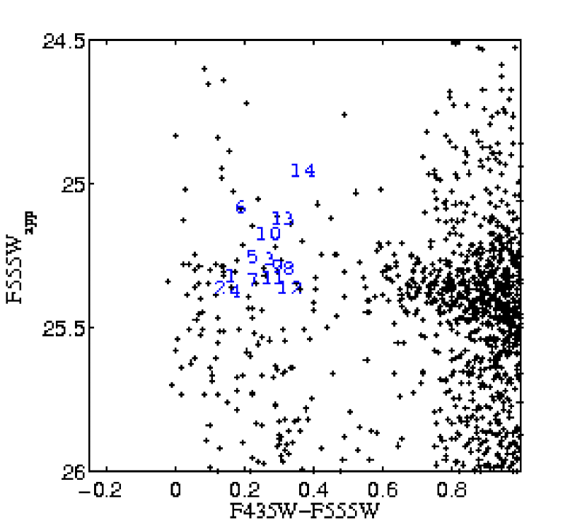
Figure 5.— As in Fig. 4, zoomed into the region of the detected RR Lyrae stars. Left: F1. Right: F2. Numbers correspond to variables listed in Tables 2 (left panel) and 3 (right panel), respectively.

Finding charts for the newly-detected RR Lyrae variables are shown in Figures 2 and 3 on the combined $F555W$ images of F1 and F2, respectively. Their locations are shown in the CMDs from M09 calibrated onto the HST VEGAMAG photometric system using the average magnitudes as reported in Tables 2 and 3 (Figure 4). We cross-correlated the RR Lyrae coordinates and magnitudes with the photometric catalog from M09 to confirm the presence of our new RR Lyrae stars in the average photometry. For all the RR Lyrae variables we found a star with same coordinates and similar magnitude (see the zoomed-in CMDs in Fig. 5).

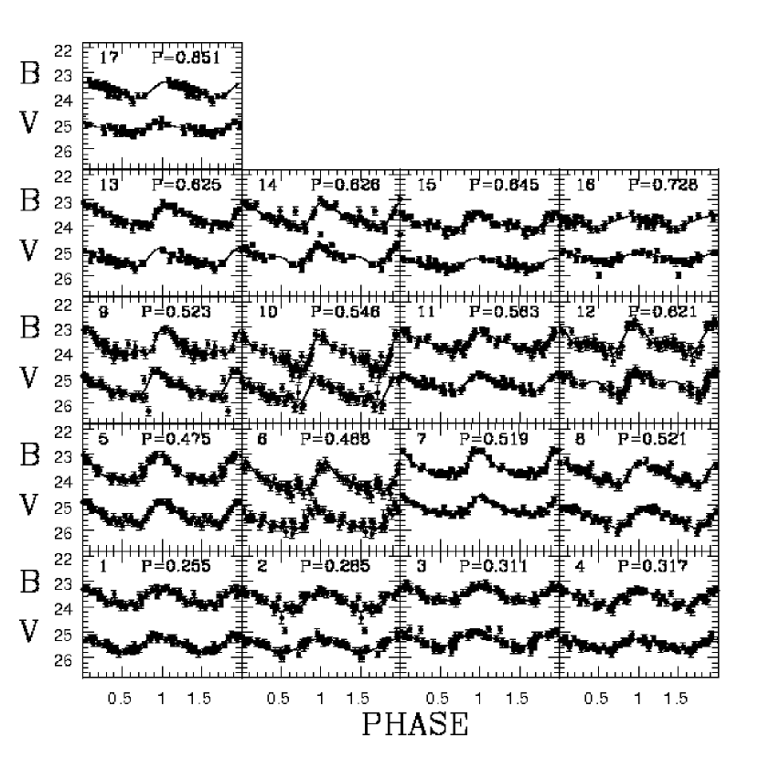
Figure 6.— Atlas of light curves in the $B$ and $V$ bands of RR Lyrae stars detected in F1. The $B$-band points have been shifted brighter by 2 mag for clarity. Error bars, as described in the text, take into account both the photometric errors as returned by DOLPHOT program as well as the scatter between the data and the model used to fit the Fourier series. The model is also shown in this Figure. For each variable star, its ID and period obtained by fitting the data points are shown in each panel as reported in columns 1 and 4 of Table 2.

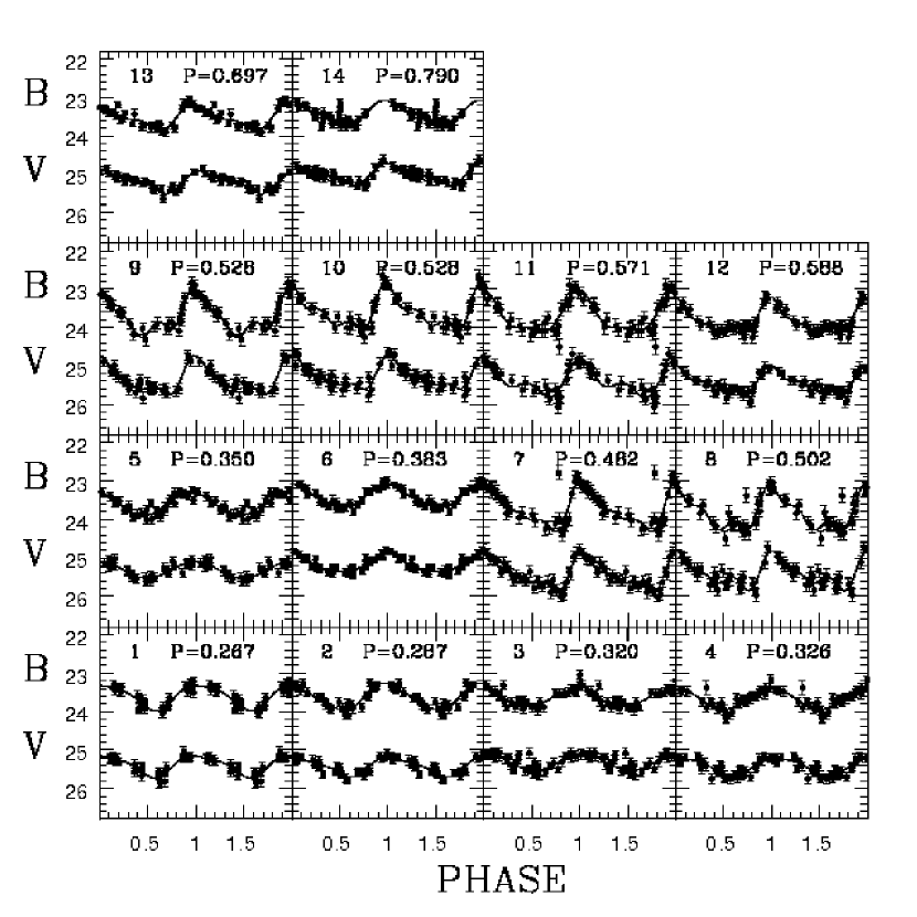
Figure 7.— As in Figure 6, but for RR Lyrae stars detected in F2.

An atlas of the light curves for all the newly-detected RR Lyrae variables is shown in Figures 6 and 7. In the atlas both data points in Johnson-Cousins system as well as the models used to perform a proper calibration onto this photometric system are shown. The error bars take into account both the scatter between the data and the model used to fit the Fourier series (see columns 13 and 14 in Tables 2 and 3) and the photometric errors as returned by DOLPHOT program. By averaging the Johnson-Cousins magnitudes we have obtained $\langle V\rangle=25.34\pm 0.15$ mag for F1 and $\langle V\rangle=25.30\pm 0.12$ mag for F2. Then, we have classified RR Lyrae variables into fundamental-mode (FU) or first-overtone (FO) pulsators by an inspection of this atlas. FO pulsators have mean periods of $\sim 0.3$ d and sinusoidal light curves, whereas the FU pulsators have longer periods ( $\langle P_{ab}\rangle=0.59\pm 0.11$ d) and more complicated light curves (with up to 4 harmonics). Because our sample of RR Lyrae variables is small, we find the same ratios of FO to FU pulsators in the two fields to within the Poisson errors: $N_{c}/N_{\mathrm{total}}=0.23^{+0.27}_{-0.23}$ and $N_{c}/N_{\mathrm{total}}=0.42^{+0.58}_{-0.25}$ for F1 and F2, respectively. We discuss the RR Lyrae properties in detail in Section 5.

Figure 8.— Spectra of the probability to detect variability in the period range from 0.2–2 d for the F1 (top) and F2 (bottom) fields observed with ACS/HRC (this paper). Note that the mean period found for F1 and F2 is $0.59\pm 0.11$ d.

Here we want to conclude by addressing an important question about the temporal completeness of these observations. That is, could we have detected all of the RR Lyrae stars in these fields at any reasonable period? To compute the probability of detecting variability with periods of 0.2–2 d, we followed the method suggested by Saha et al. (1986) and Saha & Hoessel (1990, see section IV and Figure 7 therein), using software kindly supplied by E. Bernard. We simulated one million stars randomly phased and distributed with periods of 0.2–2 days in bins of 0.001 d and then folded the Heliocentric Julian Dates of both filter datasets according to the random period and initial phase of each artificial star (see Bernard et al., 2009, for details). A variable is considered recovered if it has a) at least two observations around the maximum of the light curve, b) at least two phase points in the descending part of the light curve, and c) a minimum of three observations during the minimum light. The results are shown in Figure 8, where the probability of detecting variability is plotted as a function of the period. The computed probability for F1 and F2 is nearly unity over the entire range 0.2–0.9 days. We therefore assume a final (photometric plus temporal) completeness parameter of 100% for both fields.

4. Have We Detected M32 RR Lyrae Variable Stars?

We have clearly detected RR Lyrae variables in F1, a field dominated by M32. Are any of these stars truly associated with M32? Or does the strong background signal from M31 RR Lyrae variables (judging from F2, which is nearly free of M32 stars) dominate our detection?

We begin addressing these questions by examining the implications of our detections of RR Lyrae variables in F1 and F2 on the detection of M32 RR Lyrae variables. We then extend our analysis to include the M31 background represented by fields F2–F4 and ask this question again. Finally, we examine our results in the context of the study of Alonso-García et al. (2004), who have previously claimed detection of M32 RR Lyrae variable stars and therefore the presence of an ancient stellar population in that galaxy.

Table 5Fields near M32 with claimed RR Lyrae detections

ID	RA	DEC	Time Window	Instrument	N(RR)tot	N(RR)FU	N(RR)FO	FoV	Completeness
	(2000)	(2000)						arcmin2
F1	00:42:47.63	40:50:27.4	2005 Sep 20–24 ($\sim 24$ hr)	ACS/HRC	17	13	4	0.25	100%
F2	00:43:07.89	40:54:14.5	2006 Feb 6–12 ($\sim 24$ hr)	ACS/HRC	14	8	6	0.25	100%
F3	00:42:41.2	40:46:38	2005 Sep 22–24 ($\sim 10$ hr)	ACS/WFC	324	267	57	9	97%
F4	00:43:20.8	40:57:25	2006 Feb 9–12 ($\sim 10$ hr)	ACS/WFC	357	288	69	9	98%
F5	00:43:01	40:50:21	1998 Nov 19 ($\sim 4$ hr)	WFPC2	29	0	0	5.7	5–15%
F6	00:43:28	41:03:14	1998 Nov 20 ($\sim 4$ hr)	WFPC2	16	0	0	5.7	5–15%

4.1. M32 RR Lyrae Population Inferred from F1 and F2

Figure 9.— Probability distribution functions for the expectation value of the number RR Lyrae variable stars belonging to M32 in field F1. Left: $P(N^{\mathrm{M32,F1}}_{\mathrm{RR\ Lyrae}})=P(\mu_{F}|N_{B}+N_{F})$ [equation (4)] using only the number of RR Lyrae stars found in F1 and F2. Right: $P(N^{\mathrm{M32,F1}}_{\mathrm{RR\ Lyrae}})=P(\mu_{F}|N_{B}+N_{F})$ [equation (7)] using the number of RR Lyrae stars found in F1–F4, accounting for area differences and completeness. See text for more details.

We ask the question whether any of the RR Lyrae stars in F1 could belong to M32 given the M31 background represented by F2, or at least what the upper limit on the number of RR Lyrae stars belonging to M32 is. We have observed 14 RR Lyrae stars in F2 and 17 in F1. Our assumption is that the stellar population in F2 represents a constant background in F1. Let us call the “true” number (the expectation value) of RR Lyrae stars in each field belonging to M31 $\mu_{B}$ and the “true” number of RR Lyrae stars in F1 belonging to M32 $\mu_{F}$. What we observe is $N_{B}=14$ in F2 and $N_{B}+N_{F}=17$ in F1. Then, by Bayes’ theorem (see, e.g. Sivia & Skilling, 2006), the probability of finding some $\mu_{B}$ given $N_{B}$ is

$$P(\mu_{B}|N_{B})\propto P(N_{B}|\mu_{B})P(\mu_{B}),$$ (1)

where the constant of proportionality, $1/P(N_{B})$, can be treated as a normalization constant such that $\int P(\mu_{B}|N_{B})d\mu_{B}=1$. By the product rule, the joint probability of finding $\mu_{F}$ and $\mu_{B}$ given $N_{B}+N_{F}$ is

$$P(\mu_{F},\mu_{B}|N_{B}+N_{F})\propto P(N_{B}+N_{F}|\mu_{F},\mu_{B})P(\mu_{B}|N_{B})P(\mu_{F}),$$ (2)

where $P(\mu_{B})$ and $P(\mu_{F})$ are priors on $\mu_{B}$ and $\mu_{F}$ which we discuss below, and $P(N_{B}|\mu_{B})$ and $P(N_{B}+N_{F}|\mu_{F},\mu_{B})$ are both represented by Poisson distributions, as we are counting stars:

$$P(N|\mu)=\frac{\mu^{N}e^{-\mu}}{N!}.$$ (3)

In order to determine the probability distribution of $\mu_{F}$ given $N_{F}+N_{B}$, we need to marginalize equation (2) over $\mu_{B}$:

$$P(\mu_{F}|N_{B}+N_{F})\propto\int d\mu_{B}P(N_{B}+N_{F}|\mu_{F},\mu_{B})P(\mu_{B}|N_{B})P(\mu_{F}).$$ (4)

All that is left is to specify the priors $P(\mu_{B})$ and $P(\mu_{F})$ (and to normalize the probability distributions). Because this is a location problem (see Chap. 5 of Sivia & Skilling, 2006), we choose uniform priors, with ranges specified by the reasonable range of RR Lyrae specific frequencies $\mathrm{S_{RR}}$ given the known old populations in M32 and M31 from M09 [see equation 8 below]:

$$P(\mu)=\left\{\begin{array}[]{ll}\frac{1}{b-a}&\textrm{if $a\leq\mu\leq b$}\\ 0&\textrm{otherwise}\end{array}\right.,$$ (5)

where $a$ and $b$ define the range of reasonable values for the expectation value $\mu$. For $\mu_{F}$, we choose $a=0$ and $b=25$, and for $\mu_{B}$, we choose $a=1$ to enforce the presence of some background stars in F1 and $b=25$. These limits on the priors imply $0\leq\mathrm{S_{RR}}\leq 23$ for M32 in F1 and $1.8\leq\mathrm{S_{RR}}\leq 44$ for M31 (assuming the M31 stellar population is identical in F1 and F2) using the old, metal-poor star fractions described below. Note that we require integer numbers of stars, so the integration over $\mu_{B}$ in equation (4) becomes a sum over $\mu_{B}$, restricted by equation (5) and our choice of $a$ and $b$ to the range $1\leq\mu_{B}\leq 25$.

With this machinery in place, we find the most probable $\mu_{F}=3$ RR Lyrae stars (as expected) belonging to M32, with 68% confidence interval of 0–6 RR Lyrae stars (left panel of Fig. 9). Another way of looking at this is to assert that all the RR Lyrae variables in F2 come from M31, as stated above, so $\mu_{B}=14\pm\sqrt{14}$. Then the number of observed RR Lyrae variables in F1 is 17, so the number of RR Lyrae variables in F1 that do not come from M31 is $17-\mu_{B}=17-14\pm\sqrt{14}=3\pm 4$ (for integer numbers of stars). We therefore cannot claim to have detected RR Lyrae stars in M32 with reasonable confidence based on only F1 and F2, and we can put an upper limit of no more than 6 RR Lyrae belonging to M32 in F1 from this analysis.

4.2. M32 RR Lyrae Population Inferred from F1–F4

Figure 10.— The population of RR Lyrae stars in fields F1–F4 (see Fig. 1 for field placements). Top: RR Lyrae population (per square arcminute) as a function of the inferred M32 surface brightness (in the $V$ band). Bottom: RR Lyrae population (per square arcminute) as a function of the projected distance from M32.

Unfortunately, both fields F1 and F2 suffer from small number statistics due to the small angular size of the ACS/HRC. If we allow that F1 exceeds F2 just by chance, we should also ask if F2 exceeds the “true” background also by chance. Fields F3 and F4 may provide some guidance here, as they cover much larger areas (as they were taken with ACS/WFC) and therefore have much smaller statistical errors, as shown in Figure 10. In addition these two fields nearly fall on the same M31 isophote that passes through F1 and F2. We therefore continue our search for M32 RR Lyrae variables assuming that fields F2–F4 constitute a fair sampling of the background.

Figure 11.— Same as in Figure 8 but for the F3 and F4 fields observed with ACS/WFC and analyzed by S09. Periods found for F3 and F4 are $0.55\pm 0.07$ d and $0.56\pm 0.08$ d, respectively. These spectra are not the same as in Figure 8 due to the fact that these fields were observed for only half of the time that F1 and F2 were.

We must first consider the photometric and temporal completess of F3 and F4. S09 did not perform ASTs on these fields to calculate the completeness, but according to their luminosity function and to their comparison with Brown et al. (2004), they assume 100% photometric completeness, which we will also assume here. Using the same procedure outlined in Section 3, we can estimate the temporal completeness for these fields. Figure 11 shows the computed probability for F3 and F4, revealing a slight difference between the sampling of the two fields F3 and F4. In particular for period values around $\langle P_{ab}\rangle=0.59$ d, the probability decreases to 0.8 and 0.95 when $P=0.65$ and 0.55 d for F3 and F4, respectively. This is due to the shorter time window for these parallel fields than for the primary fields F1 and F2 (see Sec. 2.1). There are 45 (out of 324) RR Lyrae variables with periods 0.6–0.7 d (i.e., 80% temporal completeness) in F3 and 142 (out of 357) RR Lyrae variables with periods 0.5–0.6 d (i.e., 95% temporal completeness) in F4. We therefore estimate a total completeness of 97% and 98% for F3 and F4, respectively.

Now we extend our equations (1)–(5) to include all three background fields, accounting for the different areas of the background fields and F1. Because all of the background field measurements are independent, we can write the number of background counts as the sum of all three fields, corrected for completeness:

$$N_{B^{\prime}}=\sum_{i=\mathrm{F2}}^{\mathrm{F4}}\frac{N_{B_{i}}}{c_{i}}=712,$$ (6)

where $N_{B_{i}}$ is the number of stars in field $i$ and $c_{i}$ is the completeness of field $i$. Then we can write equation (4) as

$$P(\mu_{F}|N_{B}+N_{F}) \propto \int d\mu_{B}P(N_{B}+N_{F}|\mu_{F},\mu_{B})$$ (7)

$${}\times P\left(\frac{A_{B^{\prime}}}{A_{\mathrm{F1}}}\mu_{B}|N_{B^{\prime}}\right)P(\mu_{F}),$$

where $A_{B^{\prime}}/A_{\mathrm{F1}}$ is the ratio between the total area of the background fields and the area of F1, $A_{B^{\prime}}/A_{\mathrm{F1}}=\sum_{i=\mathrm{F2}}^{\mathrm{F4}}A_{B_{i}}/A_{\mathrm{F1}}=73$.

Assuming the same priors as in the previous section [equation (5) and the following discussion], we find that the number of RR Lyrae variables belonging to M32 in F1 has a most probable value of $\mu_{F}=7$, with a 68% confidence interval of 4–11 RR Lyrae variables (right panel of Fig. 9). Again, we can interpret this result as assuming that the estimated contribution from M31 RR Lyrae variables in F1 is $712/73=10$, so the inferred number of M32 RR Lyrae variable in this field is $17-10\pm\sqrt{10}=7\pm 3$ (again, for integer numbers of stars). Note that this analysis is only correct if the surface brightness of M31 is constant across fields F1–F4. We can therefore claim to have detected seven RR Lyrae variables belonging to M32 in field F1 (with a $1\sigma$ upper limit of 11 RR Lyrae stars) under this assumption. Therefore we conclude that, indeed, M32 has an ancient population as represented by the detection at 1-sigma level of RR Lyrae stars.

4.3. Specific Frequency of M32 RR Lyrae stars

We can use this number of RR Lyrae stars belonging to M32 to estimate an upper limit on the specific frequency of M32 RR Lyrae stars ($\mathrm{S_{RR}}$) in F1, assuming that its old, metal-poor population resembles that of the Galactic globular clusters. $\mathrm{S_{RR}}$ is defined as the number of RR Lyrae stars ($\mathrm{N_{RR}}$) normalized to a total Galactic globular cluster luminosity of $M_{Vt}=-7.5$ mag:

$$\mathrm{S_{RR}}=N_{RR}\,10^{(M_{Vt}+7.5)/2.5}$$ (8)

(Harris, 1996). We therefore need to obtain the luminosity of the old, metal-poor population of M32 in our field. The surface brightness of M32 in F1 is $\mu_{V}\approx 21.9\,\mathrm{mag}/\Box\arcsec$ (Kormendy et al., 2009). Assuming $E(B-V)=0.08$ (Schlegel et al., 1998) and a distance modulus $(m-M)_{0}=24.50$ (M09) we obtain a total luminosity of M32 in F1 of $M_{Vt}\sim-10$ mag. We then consider the metallicity distribution function (MDF) of M32 derived by M09, from which a 10 Gyr-old population having $-2.3<\mathrm{[Fe/H]}<-1.3$ constitutes 11% of the total luminosity. The M32 luminosity of the old, metal-poor population in F1 is thus $M_{V}=-7.6$ mag. This implies $\mathrm{S_{RR}}\approx 6.5$ for this outer region of M32, with 68% confidence limits of $3.6\leq\mathrm{S_{RR}}\leq 10$, which is in reasonable agreement with $\mathrm{S_{RR}}$ of Galactic globular clusters with metallicities $\mathrm{[Fe/H]}\sim-1.6$ (see Fig. 10 in Brown et al. 2004).

We can also estimate $\mathrm{S_{RR}}$ for the stellar population of M31 sampled in F2. The surface brightness in this field is $\mu_{V}\sim 22.7\,\mathrm{mag}/\Box\arcsec$, and assuming the same distance modulus and reddening than F1, we obtain a total luminosity of M31 in F2 of $M_{Vt}\sim-9.24$ mag. We consider again only the old, metal-poor population in F2 and calculate its luminosity. From the MDF of M31 by M09, a 10 Gyr-old population with metallicities $-2.3<\mathrm{[Fe/H]}<-1.3$ constitutes a 12% of the total luminosity, which translates into $M_{Vt}\sim-6.9$ mag. The 14 RR Lyrae stars found in F2 imply a $\mathrm{S_{RR}}\sim 18$ of M31 in this field. Note that this value is higher than $\mathrm{S_{RR}}\sim 11.2$ estimated by Brown et al. (2004) for their M31 halo field. However, the scatter in $\mathrm{S_{RR}}$ in the Galactic globular cluster system is large enough to encompass these variations if M31’s RR Lyrae population is similar to the Milky Way’s (cf. the discussion in Brown et al., 2004).

One might be tempted to attempt to invert this analysis to determine the (upper limit on the) fraction of old, metal-poor stars in M32 and M31. After all, we know the upper limit on the number of RR Lyrae stars we can associate with M32 in F1 and the number we can associate with M31 in F2. However, no theoretical or empirical one-to-one relationship between $\mathrm{S_{RR}}$ and metallicity exists, due to the scatter in this $\mathrm{S_{RR}}$–[Fe/H] plane induced by the “second-parameter problem” (see, e.g., Suntzeff et al., 1991; Brown et al., 2004). Furthermore, we have used the known fraction of metal-poor stars in M32 in F1 (and in M31 in F2) determined by M09 and a reasonable guess for the ages of these metal-poor stars to estimate $\mathrm{S_{RR}}$, so such an analysis would be circular. Alternately, if there were a stellar evolution model that correctly predicted mass-loss along the first-ascent giant branch so that the distribution of stars along the horizontal branch was also correctly predicted, we could also perform this inversion; but no such model currently exists (see, e.g., Salaris & Cassisi, 2005).

4.4. Comparison with Alonso-García et al. (2004)

Alonso-García et al. (2004) were the first to attempt to directly detect an ancient population in M32 using RR Lyrae variables. They claimed to have detected $12\pm 8$ RR Lyrae stars in a field further away from M32 than F1. From this claimed detection, they conclude that 2.3% of M32’s stellar population is old.

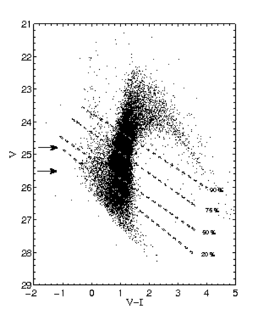
Figure 12.— The JC-calibrated ($V-I$,$V$) CMD for field F5 and various completeness levels (dashed lines). The arrows show the location where we expect to find RR Lyrae stars. On this basis we conclude that the photometric completeness is between 20 and 75%. See M09 for more details.

Figure 13.— Same as in Figure 8 but for the F5 and F6 fields observed with WFPC2 and analyzed by Alonso-García et al. (2004).

In this section, we analyze the temporal and photometric completeness of Alonso-García et al.’s data in order to determine if our detections and theirs are compatible. The authors do not give any estimate of the photometric completeness, but by examining their CMD we can see that the luminosity level of the horizontal branch is evidently at the detection limit of the WFPC2 exposures. We call their primary (“M32”) field F5 and their background (“M31”) field F6 in Table 5. M09 performed photometry and ASTs on F5 to compute their completeness levels using HSTphot (Dolphin, 2000). In Figure 12 we show the ($V-I$, $V$) CMD calibrated onto the JC photometric system using the calibrations provided by Holtzman et al. (1995). We conclude that the photometric completeness for RR Lyrae stars in F5 is 20–75%, depending strongly on color. Field F6 is similarly deep and therefore we assume that its photometric completeness is identical. Figure 13 shows that the temporal completeness computed for F5 and F6 using the method described in Section 3 is only $\approx 0.2$ for the mean period observed for RRab Lyrae ($P\sim 0.59$ days) and is 0.6–0.8 for RRc ($P\sim 0.28$–0.32 days). We stress here that the RRc detectability mostly depends on the quality of photometry due to the very low amplitudes of FO pulsators and that Alonso-García et al. (2004) likely could not have detected any of these. Thus we can assume a total (photometric and temporal) completeness for these fields of around 5–15%.

Given our own RR Lyrae detections in F1, we can estimate their completeness in a different manner. We note that their WFPC2 fields are 22.8 times larger in area than our ACS/HRC fields, but that the M32 surface brightness in F5 is $\mu^{\mathrm{M32,F5}}_{V}\sim 23.7\,\mathrm{mag}/\Box\arcsec$, about 5.2 times fainter than F1. We assumed that the M31 surface brightness is the same in both fields, $\mu^{\mathrm{M31}}_{V}\sim 22.7\,\mathrm{mag}/\Box\arcsec$. Then the total number of RR Lyrae we predict that Alonso-García et al. (2004) should have detected if they had 100% completeness, given $N_{\mathrm{M31,F1}}$ RR Lyrae variables belonging to M31 and $N_{\mathrm{M32,F1}}$ RR Lyrae variables belonging to M32 in F1, is

$$N_{\mathrm{tot,F5}}=22.8N_{\mathrm{M31,F1}}+22.8N_{\mathrm{M32,F1}}\frac{10^{-0.4\mu_{V}(\mathrm{M32,F5})}}{10^{-0.4\mu_{V}(\mathrm{M32,F1)}}}.$$ (9)

For $N_{\mathrm{M32,F1}}=7_{-3}^{+4}$ RR Lyrae variables belonging to M32 in F1, they should have detected $N_{\mathrm{tot,F5}}=258_{+55}^{-74}$ RR Lyrae in total (with fewer detected in F5 for more M32 variables in F1). They claim to have detected 22 RR Lyrae variables in F5, so we estimate their completeness to be $c_{\mathrm{F5}}=0.085_{-0.015}^{+0.034}$. Due to this severe incompleteness, Alonso-García et al. (2004) were not able to study the intrinsic properties of the stars they detected. In fact, they classified variable stars detected as RR Lyrae stars due only to their location in the CMD.

We can now compute the number of M32 stars we should have seen in F1 if Alonso-García et al. (2004) detected $12\pm 8$ RR Lyrae variables belonging to M32 in F5:

$$N_{\mathrm{RR,M32}}(\mathrm{F1})=N_{\mathrm{RR,M32}}(\mathrm{F5})\frac{A_{\mathrm{F1}}}{A_{\mathrm{F5}}}\frac{10^{-0.4\mu_{V}(\mathrm{F1})}}{10^{-0.4\mu_{V}(\mathrm{F5)}}}\frac{c_{\mathrm{F1}}}{c_{\mathrm{F5}}},$$ (10)

where $A_{\mathrm{F1}}$ and $A_{\mathrm{F5}}$ are the areas of the two fields, $\mu_{V}(\mathrm{F1})$ and $\mu_{V}(\mathrm{F5})$ are their surface brightnesses, and $c_{\mathrm{F1}}$ and $c_{\mathrm{F5}}$ are the completeness levels at the blue horizontal branch in the two fields. We assume here that this last ratio is $1/0.085$, based on the completeness estimate above. The scaling factor in this equation is then 2.7, a number which is driven mostly by the incompleteness of F5. That is, we should have seen 2.7 times as many M32 RR Lyrae variables in F1 than Alonso-García et al. (2004) saw in F5, for a total of $33\pm 22$ RR Lyrae variables predicted to belong to M32 in our field. This is a factor of 4.6 higher than the number that we claim to have detected. However, the lower 68% confidence level of this estimate just overlaps with the upper 68% confidence level of our estimate of $7_{-3}^{+4}$ RR Lyrae variables predicted to belong to M32 in F1. We can of course invert this procedure and predict how many M32 RR Lyrae variables Alonso-García et al. (2004) should have seen in F5 if our detection is correct. We predict that they should have seen $3_{-2}^{+3}$ RR Lyrae variables predicted to belong to M32 in F5, once again just in agreement (within the 68% confidence intervals) with their estimate of $12\pm 8$. We therefore suggest that it is possible that Alonso-García et al. (2004) detected bona fide M32 RR Lyrae variables in F5; but their severe incompleteness makes their detection highly uncertain.

We summarize this section by stating that considering only our ACS/HRC fields F1 and F2, we have detected $\leq 6$ RR Lyrae variable stars belonging to M32 in F1. Complementing our primary observations with our ACS/WFC parallel fields F3 and F4 allows a better determination of the likely M31 background in F1, and using this estimate, we claim to have detected $7_{-3}^{+4}$ RR Lyrae variable stars belonging to M32 in F1, with a most probable value of seven variable stars. We therefore conclude that M32 has an ancient population that can be detected without directly probing the oldest main-sequence turnoffs.

5. RR Lyrae Properties

We now ask whether we can separate the detected RR Lyrae stars belonging to the M32 and M31 stellar populations based on their intrinsic pulsation properties.

5.1. RR Lyrae Star Colors and the Pulsation Instability Strip

Figure 14.— Zoomed view of the CMD around the positions of RR Lyrae stars. Mean magnitudes have been calibrated onto the Johnson-Cousin photometric system. RR Lyrae stars from field F1 and those from F2 are displayed as filled and empty circles, respectively. FO pulsators are emphasized by using other larger circles around the symbols used. The boundaries of the pulsation Instability Strip and the relative values we adopted to draw them are indicated in each panel, namely $\mathrm{FOBE}_{\mathrm{F1}-\mathrm{F2}}=0.20$ mag (left solid line), $\mathrm{FRE}_{\mathrm{F2}}=0.40$ mag (dashed line) and $\mathrm{FRE}_{\mathrm{F1}}=0.58$ mag (right solid line). Interestingly RR Lyrae stars in F1 appear redder than the ones in F2 suggesting a large spread in metallicity in this field (see the text for details).

Does the average color of the RR Lyrae stars allow us to separate the two populations? In Figure 14 we show a blow-up of the CMDs in $V$ calibrated onto the JC photometric system. Inspecting this figure we see a clear difference in the color $(\langle B\rangle-\langle V\rangle)$ range of variables belonging to our different fields. In particular, F1 RR Lyrae colors are spread through a larger color range (0.18 mag) than those in F2.

To understand this difference in color range, we need to discuss the mechanisms driving the radial stellar pulsation. There are two main pulsation mechanisms, both related to the opacity in the stellar envelope layers where partially-ionized elements are abundant (hydrogen and neutral or singly-ionized helium): the $\kappa$- and $\gamma$- mechanisms. These are directly correlated to the variations, in these layers, of the opacity ($\kappa$) and the adiabatic exponent ($\Gamma_{3}-1$), respectively. These mechanisms can explain the pulsational instability strip (IS), the well-defined region in color where we find RR Lyrae stars and radial periodic pulsators in general (as classical and anomalous Cepheids, SX Phe variables, etc.) are observed. If a low-mass star ($M\lesssim 0.8M_{\odot}$) in the core helium- and hydrogen-shell-burning phase (the zero-age horizontal branch) crosses the IS during its evolution, it becomes a RR Lyrae variable star.

Stars bluer than the First Overtone Blue Edge (FOBE) of the IS cannot pulsate because the ionization regions (located at almost constant temperatures) are too close to the surface, and thus the stellar envelope mass is too low to effectively retain heat and act as a valve. Moving towards the red side, at lower effective temperatures, convection becomes more efficient and, at the Fundamental Red Edge (FRE), quenches the pulsation mechanism (Smith, 1995). The width of the IS is then just the color difference between the FOBE and the FRE. The FOBE location in the CMDs is well defined by theory, and we use this in Section 5.3.2 to find an independent estimate of the distance modulus (as suggested by Caputo, 1997; Caputo et al., 2000), while the position of the FRE depends on the assumptions adopted to treat the convective transport, becoming bluer as the convective efficiency is increased.

The IS depends on the initial stellar chemical composition due to the dependence of the pulsation physics on the opacity and on the hydrogen and helium partial-ionization regions. In particular the metallicity and the convection efficiency (especially for the FRE) should have the largest effects on the boundaries of the IS. As the initial stellar metallicity increases, the opacity increases, resulting in a more efficient $\kappa$-mechanism at lower effective temperature, which implies a redder FRE. The FOBE location is almost constant, as it depends essentially on the temperature of the region where helium is completely ionized (see, e.g., Walker, 1998; Caputo et al., 2000; Fiorentino et al., 2002).

In our case, shown in Figure 14, we do not see any difference in the FOBE between the fields, with $(\langle B\rangle-\langle V\rangle)_{\mathrm{FOBE}}=0.2$ mag for both fields, whereas $(\langle B\rangle-\langle V\rangle)_{\mathrm{FRE}}=0.58$ mag for F1 and $0.40$ mag for F2. This evidence could be interpreted as a suggestion that F1 RR Lyrae field stars may have a larger spread in metallicity or age than their M31 counterparts, support for two different mixes of stellar populations in field F1. Furthermore it is interestingly to note these red RR Lyrae stars (namely V6, V10, V14, V15, V16 and V17) in F1 seem to be closer to the M32 center, located as indicated by the arrow in Figure 2. Note also that the F2 RR Lyrae stars V3 (the reddest RR_c) and V7 (the bluest RR_ab) define an empirical “OR” region of the pulsation IS (see Figures 5 and in  14) where, depending on their evolutionary path, RR Lyrae stars may pulsate in both FU or FO mode.

5.1.1 RR Lyrae Reddening Evaluation

To understand whether this difference in the color spreads is intrinsic—that is, due to the metallicities or ages of the stars—or just a reddening effect, we must study the intrinsic reddening. From Schlegel et al. (1998) we know that Galactic foreground extinction in that direction is $E(B-V)=0.08\pm 0.03$ mag and is essentially the same for both fields F1 and F2. However, we must also allow for extinction from the disk of M31, in case some of the RR Lyrae variables in F1 and F2 lie behind it. In the following we will use the intrinsic properties of the RR Lyrae stars to derive the total intrinsic reddening values for both fields in two independent ways.

The first method is based on the insensitivity of $\langle(B-V)\rangle_{\mathrm{FOBE}}$ to the intrinsic properties of different RR Lyrae populations, stressed for the first time by Walker (1998). Walker presents dereddened (magnitude-averaged) $\langle(B-V)\rangle$ IS boundary colors from accurate observations of nine Galactic and LMC globular clusters covering a range in metallicity from $\mathrm{[Fe/H]}=-1.1$ to $-2.2$ dex. He concludes that the dereddened color of the blue edge is at $\langle(B-V)\rangle_{\mathrm{FOBE}}=0.18\pm 0.02$ mag, with no discernible dependence on metallicity, while the color of the red edge shows a shift of $0.04\pm 0.03$ mag. This method was also used successfully by Clementini et al. (2003) to estimate the average reddening value in LMC RR Lyrae stars. As discussed above both fields have the same FOBE color, and therefore we obtain the same estimate for their reddening. We find a reddened color of $(\langle B\rangle-\langle V\rangle)_{\mathrm{FOBE}}$$=0.20\pm 0.03$ mag for both fields, as shown in Figure 14. Thus, we infer a value of $E(B-V)=0.02\pm 0.04$ mag for both fields. Interestingly, this value of the total reddening is more than $1\sigma$ smaller than the estimate from the Schlegel et al. (1998) map, which is meant to measure the foreground reddening.

The second method was described originally by Sturch (1966). We stress here the importance of this method, as the calibration of the H i column densities with reddening is established on its basis and used by Burstein & Heiles (1978, 1982). These authors assumed an offset of $E(B-V)=0.03$ from the values found by Sturch (1966). They fixed it under the assumption that at the Galactic poles $E(B-V)=0$, as suggested by McDonald (1977) in his analysis of RR Lyrae colors and H$\beta$ indices, whereas Sturch found $E(B-V)=0.03$. With this method we derive reddening for each RRab star from the (magnitude-averaged) color at minimum light $(B-V)_{min}$ (phases between 0.5 and 0.7), the period $P_{ab}$, and the metal abundance [Fe/H] of the variables. The application of Sturch’s method requires the knowledge of the metallicity of each individual RRab. Because we do not have this information from spectroscopy of these fields, we have decided to fix the average metallicity for both field to the value $\mathrm{[Fe/H]}=-1.6$ dex, as discussed in Section 5.3.1. Sturch’s method was calibrated on Galactic field RR Lyrae stars (Sturch, 1966; Blanco, 1992) and has been used on Galactic Globular clusters (Walker, 1990, 1998) and on LMC RR Lyrae stars Clementini et al. (2003), returning, as expected, very good agreement with the H i-based reddening measurements taking into account the Burstein & Heiles (1978, 1982) extinction zero point. Walker (1992) used the following formulation of the Sturch’s method,

$$E(B-V)=(B-V)_{min}-0.336-0.24P(\mathrm{d})-0.056\mathrm{[Fe/H]},$$ (11)

where the reddening zero point has been adjusted to give $E(B-V)=0.0$ mag at the Galactic poles, and the [Fe/H] is that of the Zinn & West (1984) metallicity scale. We infer mean reddening values of $E(B-V)=0.07\pm 0.10$ mag and $0.03\pm 0.08$ mag for F1 and F2 respectively, in statistical agreement with each other and with the Schlegel et al. (1998) map. Note however that the scatter in the actual metallicities of the RR Lyraes will increase the scatter in these estimates.

Depending on the assumed method, we therefore find two different estimates of the reddening value: a) the Schlegel et al. (1998) map and the FOBE color method suggest the same reddening for both fields but different values depending on the method, 0.08 mag and 0.02 mag respectively; b) Sturch’s method suggests a reddening slightly higher for F1 field than for F2 of about 0.04 mag. Taking into account the errors on both methods we do not find any significant difference between the two evaluations as well as between the two fields.

We will discuss all these cases when determining the distance modulus: the first one assuming $E(B-V)=0.08$ for both fields by following the Schlegel et al. (1998) map, the second one assuming $E(B-V)=0.02$ mag for both fields as suggested by the FOBE method, and the third one assuming different values, e.g., $E(B-V)=0.07$ mag for F1 and $E(B-V)=0.03$ mag for F2 found using Sturch’s method. In all cases an extinction law with $R_{V}=3.1$ will be assumed.

5.2. Mean Periods, Amplitudes and Oosterhoff Types

In this section we focus our attention on their mean periods, amplitudes and Oosterhoff types (Oo types) in order to distinguish between the two populations, M32 and M31 halo (and/or outer disk) variables. Pulsational periods and amplitudes are of fundamental importance because they depend on the star structural parameters (mass, luminosity and effective temperature) and are distance- and reddening-free observables.

RR Lyrae variables found in Galactic globular clusters can be divided in two distinct classes by the mean periods of their fundamental mode pulsators: Oosterhoff type I and II (Oosterhoff, 1939). In Oosterhoff type I (OoI) Galactic globular clusters, RRab variables have average periods of $\langle P_{ab}\rangle=0.559$ d, and in Oosterhoff type II (OoII) Galactic globular clusters they have average periods of $\langle P_{ab}\rangle=0.659$ d (Clement et al., 2001), very few clusters have RRab with periods in the range of $0.58\leq\langle P_{ab}\rangle\leq 0.62$ d (the “Oosterhoff gap”). These different Galactic Oosterhoff types may have resulted from different accretion and formation processes in the Galactic halo, a hypothesis supported by the difference in metallicities found for the two types (OoII RR Lyrae are on average more metal poor than OoI RR Lyrae, with $\langle[\mathrm{Fe/H}]\rangle\approx-1.8$ and $\approx-1.2$, respectively, although with large and overlapping metallicity distributions: Szczygieł et al. 2009). The Oosterhoff dichotomy may well hold a key to the formation history of the Galactic halo, but much evidence has suggested that this dichotomy cannot support the galaxy formation scenario in which present-day dwarf spheroidal (dSph) satellite galaxies of the Milky Way are the building blocks of our Galaxy (see, e.g., Catelan, 2006). In fact the RR Lyrae variables of these dSphs as well as those of their globular clusters fall preferentially into the “Oosterhoff gap.” Furthermore, Clement et al. (2001) investigated the properties of the RR Lyrae variables in Galactic globular clusters and found that the ratio between the number of RRc and RRab stars is constant for each of the two Oosterhoff types: $N_{c}/N_{\mathrm{total}}=0.22$ for the OoI clusters and $N_{c}/N_{\mathrm{total}}=0.48$ for the OoII clusters. It is currently not clear whether the Oo dichotomy is a peculiarity of our own Galaxy; for example, the RR Lyrae stars observed in the Magellanic Clouds do not appear to follow this dichotomy (see Alcock et al., 2000, and references therein).

Brown et al. (2004) claimed that the RR Lyrae population they discovered in the M31 halo cannot be classified into either of the Oo types. They found a mean period of $\langle P_{ab}\rangle=0.60\pm 0.10$ d (in the Oo gap) but $N_{c}/N_{\mathrm{total}}=0.46$, higher than the typical value for OoI clusters (0.22). On the other hand, Clementini et al. (2009) found that one of the most luminous M31 clusters, B514, shows a peculiarity in the Oosterhoff dichotomy. They found that the mean period of 82 RRab stars is $\langle P_{ab}\rangle=0.58$ d and $N_{c}/N_{\mathrm{total}}=0.08$, suggesting an OoI type, while at the same time having a very low metallicity, $\mathrm{[Fe/H]}\sim-1.8$ (Galleti et al., 2006), suggesting an OoII type. The very low value of the $N_{c}/N_{\mathrm{total}}$ ratio in this cluster found by Clementini et al. (2009) can be explained by the incompleteness of their sample due to the intrinsically low amplitudes of RRc stars. In a recent study based on parallel observations of our program taken with ACS/WFC, S09 found $\langle P_{ab}\rangle=0.55\pm 0.07$ d and $N_{c}/N_{\mathrm{total}}=0.24$ and $\langle P_{ab}\rangle=0.56\pm 0.08$ d and $N_{c}/N_{\mathrm{total}}=0.21$ for the F3 and F4 fields (see Table 5), respectively, suggesting an OoI type classification. S09 applied the period–metallicity–amplitude relation to their large sample (almost 700 stars) and found $\mathrm{[Fe/H]}=-1.77\pm 0.06$ for both fields, similar to the Clementini et al. (2009) results.

As briefly discussed in Section 3, we find the same mean period $\langle P_{ab}\rangle=0.59\pm 0.11$ d and, within the uncertainties, the same ratios of FO to FU pulsators in the two fields: $N_{c}/N_{\mathrm{total}}=0.23^{+0.27}_{-0.23}$ and $N_{c}/N_{\mathrm{total}}=0.42^{+0.58}_{-0.25}$ for F1 and F2, respectively. The error on the mean periods is just the standard deviations of the average value computed on our very small sample of RRab Lyrae stars, i.e., 13 stars for F1 and 8 for F2, and the errors on the ratio of FO to FU pulsators reflect only Poissonian counting uncertainties.

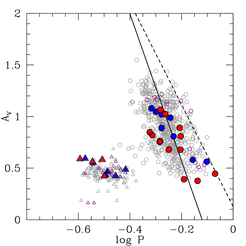
Figure 15.— Bailey Diagram ($V$-band amplitude as a function of period) for RR Lyrae stars near M32 and in the disk of M31. RR Lyrae stars in F1 are shown in red, those in F2 are shown in blue, those found by S09 in F3 and F4 are in grey, and those found in Brown et al. (2004) in F7 are in magenta. FU pulsators are circles and FO pulsators are triangles. As expected the FO pulsators are concentrated in a region with low amplitude and periods, whereas the FU pulsators show a linear behavior, i.e., their amplitudes decrease as their periods increase. That trend is stressed by the solid and dashed lines representing Oosterhoff types I and II, respectively (Clement, 2000). Nearly all FU pulsators follow the OoI relation.

We ask whether these properties are consistent with a single Oosterhoff type. In Figure 15 we show the composite Bailey diagram of Brown et al. (2004), S09, and our new detection of RR Lyrae variables. The comparison with other samples is made by assuming that their amplitudes, measured in the broad $F606W$ filter (with a peak wavelength between Johnson-Cousins the $V$ and $R$ bands), underestimate the JC $V$-band amplitudes by $\approx 8$% (for further details see Brown et al., 2004). Inspecting this figure, we see that RR Lyrae stars in both of our fields can be classified as OoI, as expected given the metallicity distribution of these fields (M09), and in particular, their lack of well-developed blue horizontal branches.

5.3. RR Lyrae Pulsation Relations

We next attempt to disentangle the putative M32 RR Lyrae population from that of the M31 using various observational manifestations of the theoretically-predicted RR Lyrae period–luminosity–temperature relation valid for every individual RR Lyrae star.

5.3.1 RR Lyrae Metallicities: [Fe/H]–Period–Amplitude Relation

To estimate the metallicity of the RR Lyrae stars in the Large Magellanic Cloud (LMC), Alcock et al. (2000) determined a relation between the metallicity [Fe/H] of an RRab variable, its period $P_{ab}$, and its $V$-band amplitude $A_{V}$,

$$\mathrm{[Fe/H]}_{ZW}=-8.85[\log P_{ab}+0.15A_{V}]-2.60,$$ (12)

where $ZW$ refers to the Zinn & West (1984) metallicity scale. This relation has been calibrated from Galactic globular clusters with metallicities in the range of $-1.4\leq\mathrm{[Fe/H]}_{ZW}\leq-2.1$ dex (and has been checked against the metallicities of Galactic field RR Lyraes). The uncertainty of this relation is $\sigma_{\mathrm{[Fe/H]}}=0.31$. This relation shows very good agreement with independent metallicity estimations for the LMC (Alcock et al., 2000), And IV (Pritzl et al., 2002), and And II (Pritzl et al., 2004). Applying this relation to the RR Lyrae variables in our two fields we find mean values of $\langle\mathrm{[Fe/H]_{F1}}\rangle=-1.52\pm 0.10\pm 0.48$ dex and $\langle\mathrm{[Fe/H]_{F2}}\rangle=-1.65\pm 0.11\pm 0.40$ dex. The first errors take into account the uncertainties of both periods and amplitudes, whereas the second errors are just the standard deviation from the mean value. There is clearly insufficient statistical evidence (given the estimated uncertainties) to conclude that we are studying two completely different populations, although the (insignificantly) higher metallicity of the RR Lyrae stars in F1 is in line with the results of M09. Note however that, as stated by Alcock et al. (2000), this relation may be affected by evolutionary effects on the RRab variables and age effects in the stellar population.

5.3.2 RR Lyrae Distance Modulus: Luminosity–Metallicity Relation and FOBE Method

Much has been written about the luminosities of horizontal branch (HB) stars (particularly their $V$-band magnitudes) and their dependence on metallicity. Recent reviews of the subject include papers by Chaboyer (1999); Cacciari (1999, 2003), and Cacciari & Clementini (2003). In this last paper, the authors describe the main properties of HB luminosities as follows:

• the relation $M_{V}(RR)=\alpha\mathrm{[Fe/H]}+\beta$ (Sandage, 1981a, b) can be considered linear, as a first approximation, with a variation of $\sim 0.25$ mag over 1 dex in metallicity;

• at a given metallicity the evolution of low mass stars from the HB produces an intrinsic magnitude spread that can reach up to $\sim 0.5$ mag. This spread can increase as the metallicity of the observed cluster increases (Sandage, 1990);

• the luminosity–metallicity relation is not strictly linear but depends on the HB morphology and is related to the “second parameter” problem (Caputo et al., 2000; Demarque et al., 2000).

RR Lyrae variables remain however excellent distance indicators once these effects are properly known and taken into account. We assume a linear $M_{V}(RR)$–[Fe/H] relation, the average of several methods:

$$M_{V}(RR)=(0.23\pm 0.04)\mathrm{[Fe/H]}+(0.93\pm 0.12)$$ (13)

(for further details see Cacciari & Clementini, 2003). To derive the distance modulus, we used this equation with observed mean magnitudes of $\langle V\rangle=25.34\pm 0.15$ mag for F1 and $\langle V\rangle=25.30\pm 0.12$ mag for F2 and a metallicity of $\mathrm{[Fe/H]}=-1.6$ dex for both fields (roughly the mean of our inferred metallicities in Sec. 5.3.1). Furthermore, we assumed different values for the reddening values as derived and discussed in Section 5.1.1:

(a)

$\mu_{0}(\mathrm{F1})=24.53\pm 0.21$ mag and $\mu_{0}(\mathrm{F2})=24.49\pm 0.19$ mag by using $E(B-V)=0.08$ mag for both fields, according to the Schlegel et al. (1998) map;

(b)

$\mu_{0}(\mathrm{F1})=24.56\pm 0.21$ mag and $\mu_{0}(\mathrm{F2})=24.64\pm 0.19$ mag by using $E(B-V)=0.07$ mag and $E(B-V)=0.03$ respectively for F1 and F2, according to the Sturch (1966) method; and

(c)

$\mu_{0}(\mathrm{F1})=24.72\pm 0.21$ mag and $\mu_{0}(\mathrm{F2})=24.59\pm 0.19$ mag by using $E(B-V)=0.02$ mag for both fields, according to the FOBE method.

The errors are conservative and take into account the scatter in the mean $\langle V\rangle$ value, metallicity uncertainties (of about 0.10 dex), and the intrinsic uncertainty in the $M_{V}(RR)$–[Fe/H] relation. Note that only taking into account for a differential reddening between the two fields (case b) can one find F1 (the field closer to M32) to be slightly closer to us than F2. As shown by S09, mostly because of the large distance of M31 from us and the relatively short distance between M31 and M32, these distance moduli do not provide any further information to disentangle the two populations. These moduli appear to be in very good agreement with estimates of both M31 ($\mu_{0}=24.44\pm 0.11$, Freedman & Madore 1990; $\mu_{0}=24.5\pm 0.1$, Brown et al. 2004; $\mu_{0}=24.47\pm 0.07$, McConnachie et al. 2005; $\mu_{0}=24.54\pm 0.07$, Saha et al. 2006; $\mu_{0}=24.46\pm 0.11$, S09) and M32 ($\mu_{0}=24.55\pm 0.08$, Tonry et al. 2001; $\mu_{0}=24.39\pm 0.08$, Jensen et al. 2003) distance moduli and with a recent estimate of the distance to M32 obtained with our data using the Red Clump method, $\mu_{0}(\mathrm{F1})=24.50\pm 0.12$ mag (M09).

Figure 16.— RR Lyrae variable stars in the $\langle V\rangle$–$\log P$ plane, where the visualization of the FOBE method is shown for an independent distance modulus (DM) determination. The symbols are the same as in Figure 14. The solid line represents the FOBE edge, by assuming a stellar mass value of $M=0.7\,M_{\odot}$ and a metallicity $\mathrm{[Fe/H]}=-1.6$. With these assumptions we find a DM of $\mu_{0}=24.56$ for a reddening value of 0.08 mag for both fields. If we assume the minimum reddening estimate of 0.02 mag as we derived (FOBE method, see Section 5.1.1), all the stars move towards fainter magnitudes an amount indicated by the arrow. In this case, we obtain a DM of $\mu_{0}=24.72$ mag (shown by the dashed line). The dotted lines represent the FOBE edges we obtained by taking into account a $0.1\,M_{\odot}$ spread in stellar mass around the initial assumed value.

The FOBE method described in Caputo (1997) and Caputo et al. (2000) provides an independent distance estimator. It is a graphical method based on the predicted period–luminosity (PL) relation for pulsators located along the first-overtone blue edge (FOBE) and seems quite robust for clusters with significant numbers of RRc variables. Using this procedure, one obtains a distribution of the cluster RR Lyrae stars in the $M_{V}$–$\log P$ plane once a distance modulus has been assumed. By matching the observed distribution of RRc variables with the following theoretical relation for the FOBE (Caputo et al., 2000),

$$M_{V}(\mathrm{FOBE}) = -0.685(\pm 0.027)-2.255\log P(\mathrm{FOBE})$$ (14)

$$\quad-1.259\log(M/M_{\odot})+0.058\log Z,$$

we can obtain an independent estimate of the distance modulus. We assume the mean metallicities derived above, $\mathrm{[Fe/H]}=-1.6$ for both fields, corresponding to $\log Z=-3.3$, and we take $M=0.7M_{\odot}$ from evolutionary HB models for RRc variables, with an uncertainty of the order of 4% (Bono et al., 2003). The FOBE method then yields a distance modulus of $\mu_{0}=24.56\pm 0.10$ mag for both fields assuming $E(B-V)=0.08$ mag. If we also take into account the minimum reddening value we obtained in Section 5.1.1 of 0.02 mag, the distance modulus increases to $\mu_{0}=24.72\pm 0.10$ mag.

5.3.3 PLC and PLC-Amplitude Relations

Figure 17.— RR Lyrae stars in the reddening-free Wesenheit plane: $\langle V\rangle-3.1\times(B-V)$ vs. $\log P$. The symbols are the same as in Figure 14. Solid and dashed lines represent the linear fits to F1 and F2 datasets respectively. The slopes of these relationships show a small but insignificant difference, as the F1 relationship is well within the $1\sigma$ and $3\sigma$ uncertainties of the F2 relation (thin dashed and dotted lines, respectively).

Figure 18.— RR Lyrae stars in the reddening-free Wesenheit plane, taking into account the $V$-band amplitudes: $\langle V\rangle-3.1\times(<B>-<V>)-\gamma A_{V}$ vs $\log P$. The symbols are the same as in Figure 14. Solid and dashed solid lines represent the fits to our data obtained with $+0.01\gamma$ and $-0.29\gamma$ values for F1 and F2, respectively. There is again an insignificant difference between the two fits, as shown in the $1\sigma$ and $3\sigma$ uncertainties for the F2 relation (thin dashed and dotted lines, respectively).

Our final attempt to disentangle the two populations is to consider at the same time all the information on the RR Lyrae variables we have obtained (including magnitudes, amplitudes, colors and periods) that reflect the individual properties of these stars. In Figures 17 and 18 we show our detected RR Lyrae stars in the reddening-free Wesenheit plane, $\langle V\rangle-R_{V}(<B>-<V>)-\gamma A_{V}$ vs period, without ($\gamma=0$) or with ($\gamma\neq 0$) taking into account a dependence on the stellar amplitudes, respectively. Because our sample of RR Lyrae variables is very small, we “fundamentalized” the first-overtone (FO) pulsators using the relation $\log P_{F}=\log P_{FO}+0.13$, where $\log P_{F}$ is the fundamentalized period (van Albada & Baker, 1973). In Figure 17 we see that both RR Lyrae groups are located in the same region; the solid and dashed lines represent the best linear fit across the data points for F1 and F2, respectively. As we can see only the slope of the relation changes, but this slope difference is statistically insignificant. The thin dashed and dotted lines represent the dispersion around the relation for F2, for $1\sigma$ and $3\sigma$ respectively. In Figure 18 we see that the periods of RR Lyrae stars in F2 do not show any dependence on their own amplitudes, whereas the periods of RR Lyrae stars in F1 show a mild dependence on their pulsation amplitudes of $\gamma=-0.19$ dex. However, the two relationships are in statistical agreement with each other, suggesting that the RR Lyrae properties of the two groups are very similar.

We summarize this section by stating that the properties of RR Lyrae variables in our two fields, F1 and F2, are statistically inseparable. The only difference we find between the two fields is in the color of the FRE, where a population of F1 RRab variables are redder than the F2 RRab variables. We suggest that these stars may in fact belong to the M32 RR Lyrae population, but the small number of detected RR Lyrae stars prevent us from making a definitive claim as to the true cause of this color difference.

6. What Have We Learned About M32, and What Do We Still Not Know?

In this paper we present ACS/HRC observations of fields near M32 (and supplemental ACS/WFC observations) to search for RR Lyrae variable stars. The detection of RR Lyrae variable stars represents the only way to obtain information about the presence of an ancient, metal-poor population ($\gtrsim 10$ Gyr and $\mathrm{[Fe/H]}\lesssim-1$ dex) in M32 from optical data not deep enough to detect the oldest MSTO stars.

We have detected 17 RR Lyrae variable stars in F1, our field closest to M32, and 14 RR Lyrae variable stars in F2, our background field in M31’s disk. We can only claim to have detected an upper limit of 6 RR Lyrae stars belonging to M32 in F1 based on these two fields alone. We can better constrain the M32 RR Lyrae population by extending our analysis to our ACS/WFC parallel fields F3 and F4 and by assuming that the M31 surface brightness is constant over these fields. With this extension, we can claim to have detected $7_{-3}^{+4}$ RR Lyrae variable stars belonging to M32 in F1, and therefore we claim that M32 has an ancient population. The implied specific frequency of RR Lyrae stars in M32 is $\mathrm{S_{RR}}\approx 6.5$, with a 68% confidence interval of $3.6\leq\mathrm{S_{RR}}\leq 10$, similar to typical intermediate-metallicity ($\mathrm{[Fe/H]}\sim-1.5$ dex) Galactic globular clusters. In making these estimates, note that we have assumed that the metal-poor population constitutes 11% of the total luminosity of M32 in F1 following the metallicity distribution function presented in M09 and further that this population has an age of 10 Gyr.

We have also used the background M31 population to infer a specific frequency of RR Lyrae variables in M31’s disk, $\mathrm{S_{RR}}\approx 18$, that is higher than the value found by Brown et al. (2004) in M31’s halo, $\mathrm{S_{RR}}\approx 11$. This may reflect merely small fluctuations in the horizontal-branch morphology with position in M31 or it may reflect some property of M31’s disk; it is difficult to state conclusively the cause without a better understanding of how the horizontal branch is populated (and therefore how mass is lost on the first-ascent giant branch).

Even though we claim to have detected bona fide M32 RR Lyrae variable stars in F1, the pulsational properties stars in fields F1 and F2 present nearly no significant differences. They have indistinguishable mean $V$ magnitudes [$\langle V\rangle=25.34\pm 0.15$ mag and $\mu_{0}=24.53\pm 0.21$ mag for F1; $\langle V\rangle=25.30\pm 0.12$ mag and $\mu_{0}=24.49\pm 0.19$ mag for F2 by assuming E(B-V)=0.08 mag and $\mathrm{[Fe/H]}=-1.6$ dex for both fields], the same mean periods ($\langle P_{ab}\rangle=0.59\pm 0.11$ d), and the same distribution in the Bailey ($V$-band amplitude–log Period) diagram, and insignificantly different ratios of RRc to RRab types ($N_{c}/N_{ab}=0.30_{-0.30}^{+0.37}$ and $N_{c}/N_{ab}=0.75_{-0.42}^{+1.25}$ respectively). By using the relation between the metallicity [Fe/H] of each RRab variable, its period $P_{ab}$, and its $V$-band amplitude $A_{V}$, we find mean values of $\langle\mathrm{[Fe/H]}\rangle_{\mathrm{F1}}=-1.52\pm 0.10$ dex and $\langle\mathrm{[Fe/H]}\rangle_{\mathrm{F2}}=-1.65\pm 0.11$ dex. We stress here that these metallicities, as well as those found by S09 ($\mathrm{[Fe/H]}=-1.77\pm 0.06$ from nearly 700 stars), are far away from the “solar-like” metallicity used by Brown et al. (2000) to interpret the UV excess they found in the core of M32 as a hot horizontal branch. However, we do find a population of F1 RRab variables that are redder than F2 RRab variables. We suggest that these stars may in fact belong to the M32 RR Lyrae population, but the small-number statistics imposed by the small ACS/HRC area makes a definitive claim difficult or even impossible.

We have detected M32’s long sought-after ancient, metal-poor population through its RR Lyrae population. But we find that this RR Lyrae population is nearly indistinguishable in its mean pulsational properties from M31, and for that matter, its specific frequency. Does this imply that M32 and M31 formed, evolved, and (likely) interacted in such a way that their ancient, metal-poor populations share some commonality? Or is this just a coincidence? We hope that further exploration of M32’s RR Lyrae population, from fields closer to the center of M32, and high-resolution spectroscopy of individual stars, revealing their detailed chemical compositions and therefore details about their formation histories, in M32 and the disk of M31 will eventually become available to help answer these questions.

References

- Alcock et al. (2000) Alcock, C., et al. 2000, AJ, 119, 2194