Negative tunnel magnetoresistance and differential conductance in transport through double quantum dots

Abstract

Spin-dependent transport through two coupled single-level quantum dots weakly connected to ferromagnetic leads with collinear magnetizations is considered theoretically. Transport characteristics, including the current, linear and nonlinear conductance, and tunnel magnetoresistance are calculated using the real-time diagrammatic technique in the parallel, serial, and intermediate geometries. The effects due to virtual tunneling processes between the two dots via the leads, associated with off-diagonal coupling matrix elements, are also considered. Negative differential conductance and negative tunnel magnetoresistance have been found in the case of serial and intermediate geometries, while no such behavior has been observed for double quantum dots coupled in parallel. It is also shown that transport characteristics strongly depend on the magnitude of the off-diagonal coupling matrix elements.

I Introduction

Transport properties of double quantum dots (DQDs) have recently attracted considerable attention from both experimental and theoretical sides. derWielRMP03 ; lossPRA98 ; hansonPRL07 ; ono02 ; graberPRB06 ; mcclurePRL07 ; golovachPRB04 ; cotaPRL05 ; aghassiPRB06 ; wunschPRB05 ; franssonPRB06 This is mainly due to the fact that DQDs are one of the simplest model systems that mimic behavior of real molecules, and are thus frequently referred to as artificial molecules. Moreover, double quantum dots are considered to play an important role in quantum computation lossPRA98 ; hansonPRL07 and spintronics. maekawa02 ; zutic04 ; maekawa06 They exhibit a variety of different phenomena, including the Pauli spin blockade, ono02 formation of molecular states, graberPRB06 spin filtering effects, cotaPRL05 or various interference effects, such as Fano or Dicke resonances. trocha ; trochaJNN In addition, very recently it was shown theoretically that, when coupled to ferromagnetic leads, double quantum dots display a considerable tunnel magnetoresistance (TMR) and spin accumulation effects. hornbergerPRB08 ; weymannPRB_DQDs ; trocha ; trocha1 Spin-dependent transport properties of quantum dots have been so far mainly addressed in the case of single quantum dots. rudzinski01 ; braunPRB04 ; cottet04 ; weymannPRB05 ; kondoSQD ; barnasJPCM08 This field is already rather well established and transport through single quantum dots coupled to ferromagnetic leads has been extensively studied experimentally. sahoo05 ; pasupathy04 ; fertAPL06 ; hamayaAPL07a ; hamayaAPL07b ; hamayaPRB08 ; parkinNL08 ; hamayaPRL09 On the other hand, theoretical investigations of spin effects in multi-dot structures are in relatively initial stage, and so is experimental implementation of DQDs coupled to ferromagnetic leads, which still remains a challenge.

In this paper we consider the spin-dependent transport properties of double quantum dots focusing on the weak coupling regime. Conductance of the system is then determined mainly by discreteness of the dots’ energy levels and Coulomb correlations, which may lead to the Coulomb blockade effect and step-like current-voltage characteristics. To calculate the transport characteristics in the linear and nonlinear response regimes, we employ the real-time diagrammatic technique. diagrams This technique allows us to take into account the interference effects resulting from virtual processes between the two quantum dots and the leads as well as renormalization of the dot levels. In particular, taking into account the first-order self-energies, we calculate the current, conductance and tunnel magnetoresistance for various geometries of the double quantum dot system. In particular, we analyze the transport characteristics in the case of DQDs connected in series, in parallel, as well as for some intermediate geometries. We show that the interference effects associated with off-diagonal matrix elements of the self-energy can significantly influence transport properties of the system for parallel and intermediate geometries. When the quantum dots are coupled in series or are in an intermediate geometry, we find negative differential conductance (NDC) and negative TMR in some transport regimes. These features appear in transport through DQD systems. However, they were not found in transport through a single quantum dot connected to ferromagnetic leads in the corresponding range of parameters. Furthermore, we also analyze the dependence of transport properties on the magnitude of the off-diagonal matrix elements. Finally, we note that in previous theoretical considerations, wunschPRB05 ; aghassiPRB06 ; weymannPRB_DQDs virtual first-order tunneling processes have not been taken into account as they become relevant for parallel and intermediate geometries of double quantum dot systems.

The paper is organized as follows. In Sec. 2 we describe the model of a double quantum dot and outline the method used in calculations. Numerical results on the current, conductance and tunnel magnetoresistance for DQDs coupled in serial, in parallel and for intermediate geometries are presented and discussed in Sec. 3. The main focus here is on negative differential conductance and negative tunnel magnetoresistance. Summary and final conclusions are given in Sec. 4.

II Theoretical description

II.1 Model

We consider two coupled single-level quantum dots connected to ferromagnetic leads, as shown schematically in Fig. 1. The magnetizations of the leads are assumed to be collinear, and the system can be either in the parallel or antiparallel magnetic configuration. The system can be switched from one configuration to the other by applying a weak external magnetic field and sweeping through the hysteresis loop, provided the leads have different coercive fields. The Hamiltonian of the double quantum dot system is generally given by

$$H=H_{\rm leads}+H_{\rm DQD}+H_{\rm tunnel},$$ (1)

where the first term, $H_{\rm leads}$, describes the left (L) and right (R) electrodes in the non-interacting quasi-particle approximation, $H_{\rm leads}=H_{\rm L}+H_{\rm R}$, with $H_{\beta}=\sum_{\mathbf{k}\sigma}\varepsilon_{\beta\mathbf{k}\sigma}c^{\dagger}_{\beta\mathbf{k}\sigma}c_{\beta\mathbf{k}\sigma}$ (for $\beta={\rm L,R}$). Here, $c^{\dagger}_{\beta\mathbf{k}\sigma}$ ($c_{\beta\mathbf{k}\sigma}$) is the creation (annihilation) operator of an electron with the wave vector $\mathbf{k}$ and spin $\sigma$ in the lead $\beta$, whereas $\varepsilon_{\beta\mathbf{k}\sigma}$ denotes the corresponding single-particle energy. The second term of the Hamiltonian describes the double quantum dot and is given by,

$$H_{\rm DQD} = \sum_{i\sigma}\limits\varepsilon_{i\sigma}d^{\dagger}_{i\sigma}d_{i\sigma}+\sum_{i}\limits U_{i}n_{i\sigma}n_{i\bar{\sigma}}$$ (2)

$$+ U_{0}(n_{1\uparrow}+n_{1\downarrow})(n_{2\uparrow}+n_{2\downarrow}),$$

where $\bar{\sigma}\equiv-\sigma$, $n_{i\sigma}=d^{\dagger}_{i\sigma}d_{i\sigma}$ is the particle number operator for spin $\sigma$ in the dot $i$ ($i=1,2$), $d^{\dagger}_{i\sigma}$ ($d_{i\sigma}$) is the respective creation (annihilation) operator, and $\varepsilon_{i\sigma}$ denotes the spin-dependent discrete energy level of the $i$-th dot. Double occupation of the dot $i$ is associated with the intradot charging energy $U_{i}$, whereas simultaneous occupation of both dots with one electron per dot costs the interdot charging energy $U_{0}$. In the following we assume $U_{1}=U_{2}\equiv U$, and note that $U_{0}<U$ for typical lateral double dot structures. derWielRMP03 We further parameterize the quantum dot energy levels by their average energy, $E_{\sigma}=(\varepsilon_{1\sigma}+\varepsilon_{2\sigma})/2$ and their difference, $\Delta E=\varepsilon_{1\sigma}-\varepsilon_{2\sigma}$, respectively, so that $\varepsilon_{1\sigma}=E_{\sigma}+\Delta E/2$ and $\varepsilon_{2\sigma}=E_{\sigma}-\Delta E/2$. Here we assumed that the dots have equal $g$-factors, then $\Delta E$ is independent of spin even in the presence of external magnetic field. Furthermore, we also assume $E_{\uparrow}=E_{\downarrow}\equiv E$, if not stated otherwise. Apart from this, we assume that the bare energy levels of the dots are independent of the applied transport voltage. This can be achieved for instance with suitable gate voltages.

The last term of the Hamiltonian, Eq. (1), consists of two different terms, $H_{\rm tunnel}=H_{\rm V}+H_{\rm t}$. The first one describes the spin-dependent tunneling processes between the quantum dots and external magnetic leads and is given by

$$H_{\rm V}=\sum_{\beta i}\sum_{\mathbf{k}\sigma}\left(V_{\beta i}c^{\dagger}_{\beta\mathbf{k}\sigma}d_{i\sigma}+V_{\beta i}^{*}d_{i\sigma}^{\dagger}c_{\beta\mathbf{k}\sigma}\right),$$ (3)

where $V_{\beta i}$ are the relevant tunneling matrix elements between the lead $\beta$ and dot $i$. The second term of $H_{\rm tunnel}$ corresponds to hopping between the two quantum dots and reads

$$H_{\rm t}=-t\sum_{\sigma}\left(d^{\dagger}_{1\sigma}d_{2\sigma}+d^{\dagger}_{2\sigma}d_{1\sigma}\right).$$ (4)

The inter-dot hopping parameter $t$ is assumed to be real and independent of the electron spin orientation. We also assume that all tunneling processes in the system are spin-conserving.

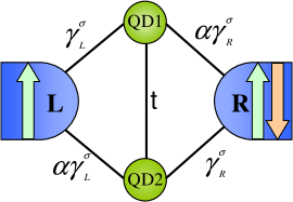
Figure 1: (Color online) Schematic picture of the DQD system coupled to ferromagnetic leads. The parameter $\gamma_{\beta}^{\sigma}$ (for $\beta=L,R,\sigma=\uparrow,\downarrow$) describes here a spin-dependent dot-lead couplings, whereas $\alpha$ takes into account difference in the coupling of a given electrode to the two dots ($\alpha\in\langle 0,1\rangle$). In particular, for $\alpha=0$ double quantum dots are in the serial geometry, while for $\alpha=1$ the system is in the parallel geometry.

Due to the coupling to external leads, the dot levels acquire finite widths. The dot-leads coupling is described generally by $\Gamma_{\beta ij}^{\sigma}=2\pi\rho_{\beta}^{\sigma}V_{\beta i}V_{\beta j}^{\ast}$, where $\rho_{\beta}^{\sigma}$ is the density of states of the lead $\beta$ for spin $\sigma$, $\sigma=+(-)$ for the majority (minority) spin electrons. $\Gamma_{\beta ij}^{\sigma}$ describes the spin-dependent hybridization between the local dot levels ($i,j=1,2$) and the leads, and is directly related to the coupling strength between the dots and leads. In principle, the coupling parameters may be energy-dependent. However, for transport regimes considered in this paper, it is well justified to assume that the couplings are constant within the electron band. wunschPRB05 For the considered system, the coupling parameters can be conveniently written in a matrix form as

$$\mathbf{\Gamma}_{\beta}^{\sigma}=\left(\begin{array}[]{cc}\Gamma^{\sigma}_{\beta 11}&\Gamma^{\sigma}_{\beta 12}\\ \Gamma^{\sigma}_{\beta 21}&\Gamma^{\sigma}_{\beta 22}\end{array}\right),$$ (5)

where the tunneling matrix elements $V_{\beta i}$ are assumed to be real and constant, while $\Gamma^{\sigma}_{\beta 12}=\Gamma^{\sigma}_{\beta 21}=q_{\beta}(\Gamma^{\sigma}_{\beta 11}\Gamma^{\sigma}_{\beta 22})^{1/2}$. The off-diagonal matrix elements of $\mathbf{\Gamma}_{\beta}^{\sigma}$ are associated with various interference effects resulting from virtual first-order tunneling processes between the two quantum dots through the states in the leads. These off-diagonal matrix elements may be significantly reduced in comparison to diagonal matrix elements $\Gamma^{\sigma}_{\beta ii}$. Furthermore, for complete destructive interference these matrix elements may be totally suppressed. To take the interference effects into account, we have introduced the parameters $q_{\rm L}$ and $q_{\rm R}$. (For calculation of the parameters $q_{L}$ and $q_{R}$ see Ref. [kubo, ].) We further assumed that $q_{\beta}$ are real positive numbers and fulfill the condition $q_{\beta}\leq 1$. Moreover, by introducing the spin polarization of lead $\beta$, $p_{\beta}=(\rho_{\beta}^{+}-\rho_{\beta}^{-})/(\rho_{\beta}^{+}+\rho_{\beta}^{-})$, the coupling constants in the parallel configuration can be simply written as

$$\mathbf{\Gamma}_{\rm L}^{\uparrow(\downarrow)}=\gamma_{L}^{\sigma}\left(\begin{array}[]{cc}1&q_{\rm L}\sqrt{\alpha}\\ q_{\rm L}\sqrt{\alpha}&\alpha\end{array}\right),$$ (6)

for the coupling to the left electrode and

$$\mathbf{\Gamma}_{\rm R}^{\uparrow(\downarrow)}=\gamma_{R}^{\sigma}\left(\begin{array}[]{cc}\alpha&q_{\rm R}\sqrt{\alpha}\\ q_{\rm R}\sqrt{\alpha}&1\end{array}\right),$$ (7)

for coupling to the right lead. In the above expressions $\gamma_{L}^{\sigma}=(1\pm p_{\rm L})\Gamma_{L}$ and $\gamma_{R}^{\sigma}=(1\pm p_{\rm R})\Gamma_{R}$. Here, we assume that the couplings are symmetric, $\Gamma_{\rm L}=\Gamma_{\rm R}\equiv\Gamma/2$, and $\alpha$ takes into account the difference in the coupling of a given electrode to the dots, see Fig. 1. In principle, the parameter $\alpha$ could be different for the left and right leads. However, we assume here that the system is symmetric, as shown in Fig.1. In the above formulas we have also assumed that in the parallel configuration the spin-$\uparrow$ (spin-$\downarrow$) electrons belong to the majority (minority) electron bands of the leads. In the antiparallel configuration the couplings are given by Eqs. (6) and (7) with $p_{\rm R}\leftrightarrow-p_{\rm R}$. By varying the parameter $\alpha$, one can change the geometry of the system from serial one for $\alpha=0$ to the parallel geometry for $\alpha=1$. For intermediate values of $\alpha$ the system is in an intermediate geometry, where each of the two dots is coupled to both leads, see Fig. 1. It is worth noting that investigating the effect of geometry on transport properties by varying the parameter $\alpha$ is certainly relevant from experimental point of view.

II.2 Method

In order to determine the transport properties of the system we employ the real-time diagrammatic technique. diagrams This technique is based on the perturbation expansion of the reduced density matrix and the relevant operators with respect to the coupling strength $\Gamma$. We calculate the reduced density matrix $\hat{\rho}$ for the double-dot system by integrating out the electronic degrees of freedom in the leads. The time evolution of $\hat{\rho}$ is then described by the Liouville equation of the form diagrams ; wunschPRB05

$$i\hbar\frac{d}{dt}\mathbf{\hat{\rho}}=[H_{\rm DQD}+H_{\rm t},\mathbf{\hat{\rho}}]+\Sigma\mathbf{\hat{\rho}}\;.$$ (8)

The commutator represents the internal dynamics in the double dot, which mainly depends on the level separation $\Delta E$ and the interdot coupling $t$. The second part of Eq. (8) accounts for the tunnel coupling between the double dot and external reservoirs. The complex tensor $\Sigma$ is associated with tunneling processes and tunnel-induced energy renormalization of the dot levels. The elements of the reduced density matrix are defined as $P^{\chi_{1}}_{\chi_{2}}\equiv\langle\chi_{1}|\mathbf{\hat{\rho}}|\chi_{2}\rangle$, where $\chi_{1}$ and $\chi_{2}$ denote the eigenstates of the DQD system. Then, the Liouville equation for stationary reduced density matrix can be written in the form diagrams

$$0=\langle\chi_{1}|[H_{\rm DQD}+H_{\rm t},\mathbf{\hat{\rho}}]\chi_{2}\rangle+\sum_{\chi_{1}^{\prime}\chi_{2}^{\prime}}\Sigma_{\chi_{2}\chi_{2}^{\prime}}^{\chi_{1}\chi_{1}^{\prime}}P^{\chi_{1}^{\prime}}_{\chi_{2}^{\prime}}\;.$$ (9)

Here, $\Sigma_{\chi_{2}\chi_{2}^{\prime}}^{\chi_{1}\chi_{1}^{\prime}}$ denotes the self-energy corresponding to evolution forward in time from state $|\chi_{1}^{\prime}\rangle$ to state $|\chi_{1}\rangle$ and then backward in time from state $|\chi_{2}\rangle$ to state $|\chi_{2}^{\prime}\rangle$. The diagonal elements of the reduced density matrix, $P^{\chi}_{\chi}$ ($\chi_{1}=\chi_{2}=\chi$), correspond to probability of finding the DQD system in the state $|\chi\rangle$. To solve Eq.9 for density matrix elements one usually performs a perturbation expansion with respect to the dot-lead coupling strength $\Gamma$. Then, each term of the expansion can be visualized graphically as a diagram defined on the Keldysh contour, where the vertices are connect by lines corresponding to tunneling processes. The self-energies in respective order of expansion can be calculated using the diagrammatic rules. diagrams

In our considerations we take into account the limit of weak tunnel coupling between the dots. For serial geometry of the double dot system, tunneling between the two dots becomes then a bottle-neck for transport and may considerably alter the spin-dependent transport characteristics of the system, as presented in the next section. This is contrary to previous theoretical studies of spin-dependent transport in DQDs, weymannPRB_DQDs where the hopping between the two dots was relatively large and transport took place through highly hybridized molecular-like states of the system. To determine transport characteristics in the weak coupling regime we perform systematic perturbation expansion with respect to the coupling parameter $\Gamma$. Furthermore, we assume $\Gamma\ll k_{B}T$. The current is then mediated mainly by first-order (sequential) tunneling processes, while the higher-order coherent tunneling events play a minor role, and it is justifiable to neglect them. wunschPRB05 ; aghassiPRB06 We thus investigate the basic transport properties using the sequential tunneling approximation, i.e. we need to determine only the lowest-order self-energies which involve one tunneling line. Some examples of first-order diagrams relevant for the present calculation are shown in the Appendix.

After calculating the density matrix elements from Eq. (9), one can determine the sequential current flowing through the double dot system from the following formula

$$I=-\frac{ie}{2\hbar}\sum_{\begin{subarray}{c}\chi_{1}\chi_{2}\\ \chi_{1}^{\prime}\chi_{2}^{\prime}\end{subarray}}{\Sigma^{\rm I}}_{\chi_{2}\chi_{2}^{\prime}}^{\chi_{1}\chi_{1}^{\prime}}P_{\chi_{2}^{\prime}}^{\chi_{1}^{\prime}},$$ (10)

where ${\Sigma^{\rm I}}_{\chi_{2}\chi_{2}^{\prime}}^{\chi_{1}\chi_{1}^{\prime}}$ denotes the first-order self-energy in which one vertex was substituted by a vertex representing the current operator, $\hat{I}=(\hat{I}_{R}-\hat{I}_{L})/2$, with $\hat{I}_{\beta}=-i(e/\hbar)\sum_{i}\sum_{\mathbf{k}\sigma}(V_{\beta i}c^{\dagger}_{\beta\mathbf{k}\sigma}d_{i\sigma}-V_{\beta i}^{*}d_{i\sigma}^{\dagger}c_{\beta\mathbf{k}\sigma})$.

In our analysis we assume that the intra-dot charging energy $U$ is relatively large for both dots, much larger than the interdot Coulomb correlation energy $U_{0}$. Thus, only the zero, one and two-particle DQD states are relevant for transport. Furthermore, in the case of $U\gg U_{0}$, the occupation probability of the states with two electrons in the same dot is also vanishingly small. However, these states are taken into account as intermediate (virtual) states in the calculation, providing a natural high-energy cutoff. Finally, we would like to emphasize that by using the real-time diagrammatic technique we are able to take into account the first-order virtual tunneling processes between the two dots in a fully systematic way. diagrams ; wunschPRB05

III Numerical results

In this section we present and discuss numerical results on the charge current, differential conductance and tunnel magnetoresistance of double quantum dots coupled in serial, parallel, and intermediate geometries. The TMR effect results generally from spin-dependent dot-lead tunneling processes, which in turn leads to the dependence of transport characteristics on magnetic configuration of the system. The TMR is quantitatively described by the ratio ${\rm TMR}=(I_{\rm P}-I_{\rm AP})/I_{\rm AP}$, where $I_{\rm P}$ and $I_{\rm AP}$ denote the currents flowing through the system in the parallel and antiparallel magnetic configurations, respectively. julliere75 ; barnas98

In the numerical analysis we assume spin degenerate dot levels, $\varepsilon_{i\sigma}=\varepsilon_{i}$ (for $i=1,2$ and $\sigma=\uparrow,\downarrow$). We also assume that external electrodes are made of the same ferromagnetic material, $p_{L}=p_{R}\equiv p$, and that the system is symmetrically coupled to the leads, $\Gamma_{\rm L}=\Gamma_{\rm R}\equiv\Gamma/2$. The parameters $q_{\rm L}$ and $q_{\rm R}$ can be generally different. However, we assume that they are real and equal, $q_{\rm L}=q_{\rm R}\equiv q$. We also set the intra- and inter-dot Coulomb parameters to be: $U=100k_{B}T$ and $U_{0}=20k_{B}T$, respectively. Finally, we assume spin polarization $p=0.4$, which is typical of 3d ferromagnetic metals. Soulen98 The inter-dot hopping parameter $t$ is assumed to be: $t=0.25\Gamma$ with $\Gamma=5\mu$eV. These are typical experimental parameters for double quantum dot systems. ono02 ; derWielRMP03 Chemical potentials of the left and right leads are set to be $\mu_{L}=eV/2$ and $\mu_{R}=-eV/2$, where $eV=\mu_{L}-\mu_{R}$ denotes the applied bias voltage.

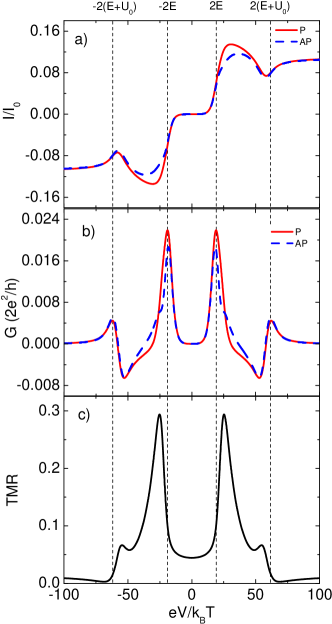
Figure 2: (Color online) Current (a) and differential conductance (b) in the parallel (P, solid line) and antiparallel (AP, dashed line) magnetic configurations, as well as tunnel magnetoresistance (c), calculated as a function of the bias voltage for the parameters: $E=10k_{B}T$, $\Delta E=0$, $U_{0}=20k_{B}T$, $U=100k_{B}T$, $p=0.4$, $t=0.25\Gamma$, $\Gamma=5\mu$eV, $\alpha=0$, and $I_{0}=e\Gamma/\hbar\approx 1.215$ nA.

III.1 Double dots connected in series, $\alpha=0$

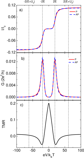
Figure 3: (Color online) Current (a) and differential conductance (b) in the parallel (solid line) and antiparallel (dashed line) magnetic configurations, and tunnel magnetoresistance (c), calculated as a function of the bias voltage for $E=-10k_{B}T$. The other parameters are the same as in Fig. 2.

Let us first consider the situation when $\alpha=0$, which corresponds to serial geometry of the double quantum dot system, see Fig. 1. In Fig. 2 we show the basic transport characteristics for the average dot level $E=10k_{B}T$ and the difference between bare dots’ levels $\Delta E=0$. In the weak coupling regime transport is determined mainly by discreteness of the energy dot spectrum and Coulomb correlations, which lead to staircase-like current-voltage characteristics, see Fig. 2(a). For the assumed parameters, the DQD is empty at low bias and the current is blocked below the threshold voltage, irrespective of magnetic configuration of the system. In the blockade regime, however, the first-order processes can still contribute to the current due to thermal fluctuations. Furthermore, in the case of $\Gamma\ll k_{B}T$, as considered in this paper, the contribution from first-order processes can still be larger than that from second-order tunneling (cotunneling). Nevertheless, one must bear in mind that in the case of deep Coulomb blockade, for instance for $E/k_{B}T\ll 0$ and $(E+U_{0})/k_{B}T\gg 0$, the second-order processes become dominant and must be taken into account to properly describe transport properties of the system. weymannPRB_DQDs In this paper, however, we restrict ourselves to the case when transport is mainly governed by sequential tunneling processes.

When the bias voltage approaches the threshold voltage, the sequential current starts to flow due to one-by-one electron tunneling through singly-occupied DQD states. This leads to the peak in the differential conductance, see Fig. 2(b). However, when the bias voltage increases further, instead of a plateau one observes a drop of the current, which leads to negative differential conductance. This feature appears in both magnetic configurations, see Fig. 2(b). When $eV$ approaches $2E+2U_{0}$, where another electron has possibility to tunnel into the DQD system, the current starts increasing further.

Physical mechanism responsible for the occurrence of negative differential conductance follows from the level renormalization due to tunneling processes between the dots and leads. This renormalization is directly related to the real part of the off-diagonal self-energies, see Eq. (A) (and also Ref. [wunschPRB05, ], where the level renormalization in a DQD system connected in series and coupled to nonmagnetic leads was calculated). Accordingly, the renormalized level $\varepsilon_{i}^{\rm ren,\sigma}$ of the $i$th dot for spin $\sigma$ has the following form:

$$\varepsilon_{i}^{\rm ren,\sigma} = \varepsilon_{i}+\Omega_{\alpha i}^{\sigma}(E)+\Omega_{\alpha i}^{\sigma}(E+U)$$ (11)

$$- \Omega_{\alpha i}^{\uparrow}(E+U_{0})-\Omega_{\alpha i}^{\downarrow}(E+U_{0})\,,$$

with $\Omega_{\beta i}^{\sigma}(x)=(\Gamma_{\beta ii}^{\sigma}/2\pi)\left[{\rm Re}\Psi\left(\frac{1}{2}+i\frac{x-\mu_{\beta}}{2\pi k_{B}T}\right)\right]$, where $\Psi(x)$ is the digamma function. This renormalization lifts the initially assumed degeneracy of the two dot’s levels. The larger separation between these renormalized levels, the smaller probability of electron tunneling from the left to the right dot. We have calculated this separation as a function of the bias voltage (not shown) and found that the separation increases with increasing bias voltage (in the voltage range where negative differential conductance appears), and therefore the current decreases with increasing bias. After reaching maximum, the level separation starts to decrease with a further increase in voltage and negative differential conductance disappears. It is also worth noting that, due to the coupling to ferromagnetic leads, the level renormalization becomes spin dependent and, consequently, depends on magnetic configuration of the system, and so does the level spacing.

The above described level renormalization makes the occupation probability of the left dot (QD1) for $eV>E$ larger than the occupation probability of the right dot (QD2), $P_{|\sigma,0\rangle}>P_{|0,\sigma\rangle}$ for $\sigma=\uparrow,\downarrow$. Moreover, the rate for tunneling between the two dots decreases with increasing the bias voltage. More specifically, ${\rm Im}\langle 0,\sigma|\mathbf{\hat{\rho}}|\sigma,0\rangle$ decreases, whereas ${\rm Im}\langle\sigma,0|\mathbf{\hat{\rho}}|0,\sigma\rangle$ increases, $\langle\sigma,0|\mathbf{\hat{\rho}}|0,\sigma\rangle=(\langle 0,\sigma|\mathbf{\hat{\rho}}|\sigma,0\rangle)^{\ast}$. In the case of tunneling through double quantum dots connected in series, the imaginary parts of the density matrix, e.g. $\langle 0,\sigma|\mathbf{\hat{\rho}}|\sigma,0\rangle$ and $\langle\sigma,0|\mathbf{\hat{\rho}}|0,\sigma\rangle$, are related to the charge transfer through the system, i.e. they are directly related to the current flow. wunschPRB05 Consequently, the tunneling of electrons from the left lead to the left quantum dot (QD1) is partially suppressed because of $P_{|\sigma,0\rangle}>P_{|0,\sigma\rangle}$ and due to decreased tunneling rates between the two dots with increasing bias voltage $V$ in the range $|eV|\in(2E,2E+2U_{0})$.

The tunnel magnetoresistance as a function of applied bias voltage is plotted in Fig. 2(c). Since the conductance is larger in the parallel configuration than in the antiparallel one, the corresponding TMR is positive, although very small in the voltage range where double occupancy is allowed. Moreover, one can note that the sequential tunneling TMR is generally smaller than the Julliere’s value of TMR, julliere75 $\rm{TMR}^{Jull}=2p^{2}/(1-p^{2})\approx 0.38$ for $p=0.4$, which is characteristic of single tunnel junction or fully coherent transport. weymannPRB05 In the case shown in Fig. 2(c), the TMR reaches local maxima for $|eV|=2E$ and for $|eV|=2E+2U_{0}$, but it is especially enhanced at the first Coulomb step, i.e. in the vicinity of $|eV|=2E$.

In Fig. 3 we present results obtained for DQD connected in series with average double dot level position being negative $E=-10k_{B}T$. The DQD system is then singly occupied in equilibrium, and the system is in the Coulomb blockade regime as double occupation of DQD would cost the correlation energy $U_{0}$. Since the levels corresponding to $E$ and $E+U_{0}$ start contributing to current at the same bias ($E$ and $E+U_{0}$ are symmetric with respect to the zero bias voltage), only one step is observed in the bias dependence of current. Contrary to the case presented in Fig. 2, now the current is a monotonic function of the applied bias voltage, and negative differential conductance is not observed, see Fig. 3(a) and (b). The difference between the two magnetic configurations is only slightly visible in the current and differential conductance. Accordingly, the TMR above the threshold voltage is very small, see Fig. 3(c). At the zero bias, however, TMR exhibits a sharp maximum and then drops with increasing bias voltage. Furthermore, for voltages around the resonance $|eV|\approx 2E$ a negative TMR is observed.

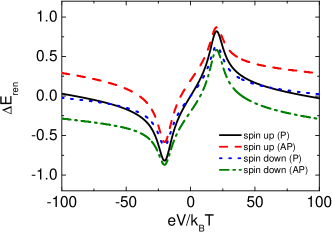
Figure 4: (Color online) Renormalization of the dots’ levels spacing for both spin orientations in the parallel and antiparallel magnetic configurations. The parameters are the same as in Fig. 3.

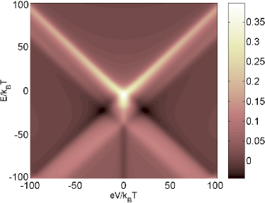
Figure 5: (Color online) Tunnel magnetoresistance as a function of the bias voltage and the average level position. The other parameters as in Fig. 3.

Physical origin of the negative TMR is similar to that of negative differential conductance discussed above. More specifically, negative TMR follows from the level renormalization due to coupling of the dots to external leads in the presence of inter-dot Coulomb correlations. This level renormalization is spin dependent, so that it lifts spin degeneracy of the dot levels. More importantly, it is generally different for each dot and therefore modifies the renormalized level spacing $\Delta E_{\rm ren,\sigma}=\varepsilon_{1}^{\rm ren,\sigma}-\varepsilon_{2}^{\rm ren,\sigma}$. The renormalization of the level spacing in the system under consideration is displayed in Fig. 4. For the assumed parameters hopping between the dots is like a bottle neck for electrons, that controls current flowing through the system. As already stated above, this hopping probability decreases with increasing level separation (for each spin orientation). When comparing Fig. 3(c) and Fig. 4, one can note that the minimum in (negative) TMR appears in the voltage range where the level spacings are maximum. Let us consider in more details positive bias, $eV>0$. In the region where negative TMR is observed, the level spacing between left and right dots for the dominant transport channel (spin-up) in the parallel magnetic configuration is significantly larger than that for spin-down electrons in the parallel configuration and also significantly larger than the spacing for one of the spin channels in the antiparallel configuration, while it is comparable to the level spacing for second spin channel in the antiparallel configuration. Thus, in the parallel configuration the spin-down channel, which involves spin-minority bands in both leads, takes over control of the current, while the dominant spin channel in the antiparallel configuration involves one spin-majority and one spin-minority bands. Consequently, the current is then larger in the antiparallel configuration than in the parallel one, which results in negative TMR.

To support this, we have calculated the relevant occupation probabilities. We have found that the occupation probability of the left dot by a spin-up electron in the parallel configuration is larger than that for the antiparallel configuration configuration, $P^{P}_{L\uparrow}>P^{AP}_{L\uparrow}$, whereas opposite relation holds for spin-down electrons, $P^{P}_{L\downarrow}<P^{AP}_{L\downarrow}$. This situation is opposite to that found for the bias region where large positive TMR appears. Moreover, the occupation probabilities of the right dot by a spin-up or spin-down electron in both magnetic configurations are small in comparison with those for the left dot. Finally, the probability of double occupation of the DQD system is rather small, consequently such states are rather irrelevant.

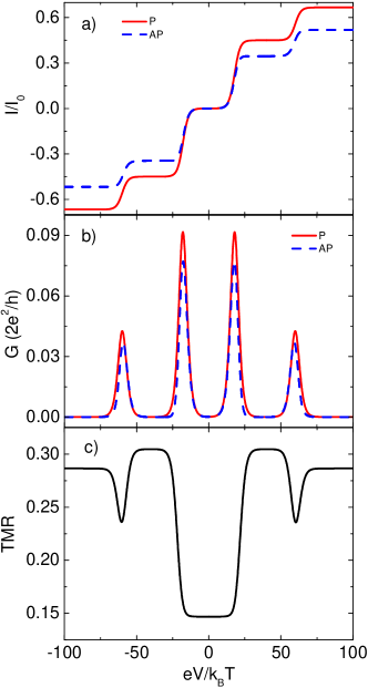
Figure 6: (Color online) The current (a), differential conductance (b) in the parallel (solid line) and antiparallel (dashed line) configurations, and tunnel magnetoresistance (c) as a function of the bias voltage obtained for the parameters: $\alpha=1$, $q=0.25$, $E=10k_{B}T$, while the other parameters are as in Fig. 2.

In Fig. 5 we show the bias voltage and level position dependence of the TMR. The position of the average level can be changed experimentally by sweeping the gate voltage, so that Fig. 5 effectively shows the bias and gate voltage dependence of TMR. One can note that as the absolute value of the average level position increases, the central maximum in TMR becomes split into two components, while the maximum at zero bias changes into a minimum. In the case of negative $E$, the minimum at zero bias occurs roughly when $E\lesssim-U_{0}$. Furthermore, there are also transport regions where TMR changes sign and becomes negative. The negative TMR occurs mainly for $E\approx-U_{0}/2$ and $|eV|\approx 2E$. One can also note that generally TMR becomes much suppressed for larger bias voltages, being close to zero, see also Figs. 2(c) and 3(c). This implies that the spin polarization of tunneling electrons is significantly reduced. Such a behavior is opposite to that in the case of two strongly coupled dots, where TMR in the sequential tunneling regime was found to be considerable. weymannPRB_DQDs

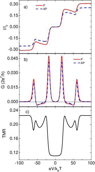
Figure 7: (Color online) Current (a) and differential conductance (b) in the parallel (solid line) and antiparallel (dashed line) magnetic configurations, and tunnel magnetoresistance (c), calculated as a function of the bias voltage for $\alpha=0.25$. The other parameters are the same as in Fig. 6.

III.2 Double dots connected in parallel, $\alpha=1$

In this subsection we consider the case when the dots are connected in parallel, $\alpha=1$, see Fig. 1. Virtual tunneling processes between the two quantum dots through the leads are now allowed. As mentioned earlier, the off-diagonal matrix elements of $\mathbf{\Gamma}_{\beta}^{\sigma}$ may be significantly reduced due to suppression/cancellation of different contributions, and hence $q<1$ in general. In the following we assume $q=0.25$. However, we will also analyze how the transport characteristics depend on the parameter $q$. For a given $q$ we will examine two cases: symmetric case when all dot-lead couplings are the same for given spin, i.e., $\alpha=1$, and asymmetric case when there is a difference in the coupling of a given electrode to the two dots, $\alpha\neq 0,1$. The latter case, referred to as the intermediate geometry, will be analyzed in the next subsection.

The current, differential conductance and TMR for the case when the DQD is empty at equilibrium, $E>0$, are shown in Fig. 6. The current exhibits a typical staircase-like behavior [Fig. 6(a)], which is also reflected in well-defined peaks in the differential conductance located at the positions $|eV|=2E$ and $|eV|=2E+2U_{0}$, see Fig. 6(b). The TMR is positive in the whole bias range and takes well-defined values corresponding to different steps in the current-voltage characteristics, see Fig. 6(c). In the case of DQD coupled in parallel, the TMR is generally larger than in the case of serial connection discussed in the previous subsection, especially for large voltages. This is due to a different role of interdot hopping in these two geometries. As the hopping term is crucial for transport in serial geometry, it plays a less important role in the parallel geometry. Since the hopping parameter is independent of spin orientation, it leads to a reduction of TMR in the serial geometry in comparison to that in the parallel one, especially at large voltages.

III.3 Double dots in a general (intermediate) geometry

The situation changes considerably when the dot-lead couplings are different, $\alpha\neq 1$, see Fig. 1. Figure 7 presents the current, differential conductance and TMR as a function of bias voltage, calculated for $\alpha=0.25$. As one can note, the shape of curves describing current and differential conductance reveals features obtained above for dots connected in series, see Fig. 2, i.e. the negative differential conductance and associated non-typical Coulomb steps in current. However, the bias dependence of TMR is now different and is more similar to that obtained for parallel geometry, except for voltages $2E<|eV|<2E+2U_{0}$, i.e. between the resonances, where the behavior of TMR is more complex and where one finds some oscillations in TMR. Furthermore, for the intermediate geometry, the TMR for larger bias voltages is quite significant, contrary to the case of serial geometry, see Figs. 2(c) and 3(c), and is only a little smaller than that in the parallel geometry, see Fig. 6.

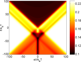
Figure 8: (Color online) Tunnel magnetoresistance as a function of the bias voltage and the average level position, calculated for $\alpha=0.25$. The other parameters are the same as in Fig. 7.

For completeness, in Fig. 8 we show the bias and gate voltage dependence of the TMR. One can see that TMR displays well defined structures consisting of regions where it is roughly constant. In these transport regions the corresponding current-voltage curves display plateaus, whereas at resonances the corresponding TMR changes considerably.

It is interesting to analyze how TMR depends on the asymmetry factor $\alpha$. In Fig. 9 we present the bias dependence of TMR calculated for different values of $\alpha$ and for the case when off-diagonal matrix elements $\Gamma_{\beta 12}^{\sigma}$ are zero ($q=0$) and finite ($q=0.25$), see Fig. 9(a) and (b), respectively. By changing $\alpha$ from $0$ to $1$, geometry of the system continuously changes from serial to parallel one. Furthermore, with increasing $\alpha$ also the magnitude of the off-diagonal matrix elements is increased, see Eqs. (6) and (7). First of all, one can note that TMR generally increases with increasing $\alpha$. This is associated with the fact that for $\alpha\neq 0$ the electrons can tunnel between the leads through just a single dot. Accordingly, the role of interdot hopping, which is independent of electron spin and therefore reduces TMR, is diminished and TMR increases. In particular, when crossing over from the serial to parallel geometry, the TMR at zero bias increases, while sharp maxima in TMR at resonance voltages are transformed into plateaus. This behavior can be observed in the case of $q=0$ and $q=0.25$, see Fig. 9(a) and (b), respectively. There are however some differences between these two situations. The virtual tunneling processes between the two dots, described by the nonzero parameter $q$, decrease the TMR at the zero bias and increase it for large bias voltages, $|eV|>2E+2U_{0}$, as compared to the case of $q=0$.

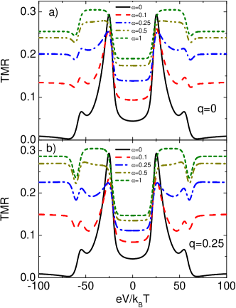
Figure 9: (Color online) Bias voltage dependence of TMR for indicated values of the asymmetry parameter $\alpha$ and for $q=0$ (a) and $q=0.25$ (b), calculated for $E=10k_{B}T$. The other parameters are the same as in Fig. 2.

Another interesting feature visible in Fig. 9 is that TMR for $\alpha=1$ at the side plateaus, i.e. for $2E+2U_{0}>|eV|>2E$, has the same magnitude for both $q=0$ and $q=0.25$ cases. This can be clearly shown by deriving an approximate analytical formula for TMR in this voltage region. At very low temperatures one can approximate the Fermi functions by step functions and assume that the electrons tunnel only from one side to the other. weymannJPCM07 Then, one can show that the TMR for $\alpha=1$ and $2E+2U_{0}>|eV|>2E$ is given by

$${\rm TMR}=\frac{8p^{2}}{5(1-p^{2})}\;,$$ (12)

which is exact at zero temperature. From the above formula follows that TMR in the bias regime under consideration is independent of the magnitude of the off-diagonal matrix elements. This is, however, not true for the current, which for $\alpha=1$ is given by

$$I^{\rm P}=\frac{e\Gamma}{\hbar}\frac{2+q}{5}\;,$$ (13)

in the parallel and

$$I^{\rm AP}=\frac{e\Gamma}{\hbar}\frac{(2+q)(1-p^{2})}{5+3p^{2}}\;,$$ (14)

in the antiparallel magnetic configurations.

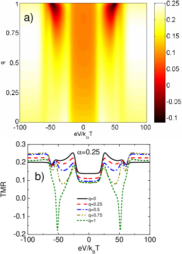
Figure 10: (Color online) (a) Tunnel magnetoresistance as a function of the bias voltage and parameter $q$, calculated for for $\alpha=0.25$. (b) Cross-sections of TMR for several values of $q$ as indicated in the figure. The other parameters are the same as in Fig. 6.

The interference effects due to virtual first-order processes between the two dots can significantly affect TMR, especially for larger values of $q$. This is shown in Fig. 10, which depicts TMR as a function of the bias voltage and parameter $q$, together with various cross-sections. It can be seen that with increasing the magnitude of the off-diagonal matrix elements, the TMR generally increases in the low bias voltage regime, $|eV|<2E$, and for larger voltages, $|eV|>2E+2U_{0}$, although the latter dependence is not monotonic. However, for bias voltages where transport occurs through charge states with single electron on the double dot, $2E+2U_{0}>|eV|>2E$, TMR becomes suppressed with raising $q$, and for $q=1$ we find a negative TMR effect. The negative TMR develops approximately at the resonance, $|eV|\approx 2E+2U_{0}$, where two-particle states of the double dot system start taking part in transport.

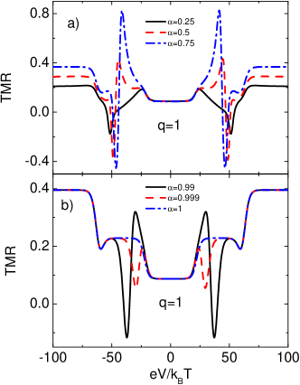
Figure 11: (Color online) Bias voltage dependence of TMR calculated for $q=1$ and for different values of the asymmetry parameter $\alpha$, as indicated in the figure. The other parameters are the same as in Fig. 2.

Figure 10 was calculated for $\alpha=0.25$. However, it turns our that the spin-dependent transport properties may also strongly depend on the geometry of the system. This is especially visible in TMR for maximum value of the parameter $q$, $q=1$. In Fig. 11 we plot TMR as a function of the bias voltage for different values of $\alpha$ and for $q=1$. As one can note, TMR is rather independent of $\alpha$ at low bias voltages, while for larger bias, $|eV|>2E+2U_{0}$, TMR generally increases with raising $\alpha$. This is however not the case for $2E+2U_{0}>|eV|>2E$, where TMR strongly depends on the geometry of the system. With crossing over from serial to parallel geometry, the magnitude of negative TMR is increased and additional maximum develops next to the resonance, $|eV|\approx 2E+2U_{0}$, which transforms into plateau for $\alpha$ close to 1.

Interestingly, it can be also seen that tunnel magnetoresistance is very sensitive to slight changes in the asymmetry parameter $\alpha$, when the latter is close to unity. To understand this behavior one needs to realize that the bare states of the two quantum dots coupled directly (by the hopping term) or indirectly (due to off-diagonal coupling matrix elements) hybridize in molecular-like states. As a result, the bonding and anti-bonding states emerge, the widths of which strongly depend on the dot-lead coupling strengths and geometry of the system. In the case considered here, the relative width of the bonding and anti-bonding states varies with the parameter $\alpha$. When the difference in the coupling of a given electrode to the two dots is reduced, the width of the bonding state increases whereas that of the anti-bonding state decreases. In particular, in the limit of $\alpha=1$, the anti-bonding state becomes totally decoupled from the leads, while the bonding state acquires width of the order of $2\Gamma$. In this limit the above mentioned features of the TMR disappear and tunnel magnetoresistance is constant for $2E+2U_{0}>|eV|>2E$. In other words, the high sensitivity of the TMR with respect to the system’s geometry is associated with the fact that the interference conditions for electron waves transmitted through the two dots become modified when changing $\alpha$.

IV Summary and conclusions

We have analyzed the spin-polarized transport properties of double quantum dots weakly coupled to each other and to external leads. Using the real-time diagrammatic technique we have calculated the conductance and tunnel magnetoresistance in the parallel, serial and intermediate geometries of double quantum dots. Moreover, we have taken into account the effects of virtual tunneling processes between the two dots taking place through the states in the leads. Such processes are absent in serial geometry and become maximum for parallel geometry.

In the case of double quantum dots coupled in series we have found a negative tunnel magnetoresistance at the resonance and negative differential conductance for transport voltages where single-particle double-dot states take part in transport. On the other hand, for parallel geometry of the system, both the negative TMR and negative differential conductance vanish. The above effects may be restored in an intermediate geometry and strongly depend on the magnitude of the virtual processes between the two dots. Furthermore, in the case when virtual processes are maximal, we have found a strong dependence of the TMR on the geometry of the system, especially for geometries very close to the parallel one.

Appendix A Examples of the first-order self energies

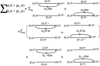
Figure 12: Graphical representation of the self-energy $\Sigma^{|\sigma,0\rangle|\sigma,0\rangle}_{|0,\sigma\rangle|0,\sigma\rangle}$ (a). The summations are over lead and spin degrees of freedom $\alpha=L,R$ and $\sigma^{\prime}=\uparrow,\downarrow$. Each tunneling line carries lead index $\alpha$, spin $\sigma$ and frequency $\omega$.

In order to analyze the transport properties one needs to calculate the respective self-energies using corresponding diagrammatic rules. diagrams ; weymannPRB05 In the sequential tunneling regime only the first-order self-energies determine the transport characteristics. Here, we present explicitly two examples of first-order self-energies. Generally, the self-energies are complex – their imaginary part may be related to transition rates, whereas the real part may be associated with with various renormalization effects. The graphical representation of the self-energy $\Sigma^{|\sigma,0\rangle|\sigma,0\rangle}_{|0,\sigma\rangle|0,\sigma\rangle}$ is displayed in Fig. 12, while analytically it is given by

$$\Sigma^{|\sigma,0\rangle|\sigma,0\rangle}_{|0,\sigma\rangle|0,\sigma\rangle} = \sum_{\alpha,\sigma^{\prime}}\left\{P^{-,\sigma}_{\alpha_{22}}({\varepsilon_{1\sigma}})-P^{-,\sigma}_{\alpha_{11}}(\varepsilon_{2\sigma})+P^{+,\sigma^{\prime}}_{\alpha_{22}}({\varepsilon_{1\sigma}+\varepsilon_{2\sigma^{\prime}}+U_{0}-\varepsilon_{2\sigma}})-P^{+,\sigma^{\prime}}_{\alpha_{11}}(\varepsilon_{1\sigma^{\prime}}+\varepsilon_{2\sigma}+U_{0}-\varepsilon_{1\sigma})\right.$$ (15)

$$+P^{+,\bar{\sigma}}_{\alpha_{11}}(\varepsilon_{1\sigma}+\varepsilon_{1\bar{\sigma}}+U_{1}-\varepsilon_{2\sigma})-P^{+,\bar{\sigma}}_{\alpha_{22}}(\varepsilon_{2\sigma}+\varepsilon_{2\bar{\sigma}}+U_{2}-\varepsilon_{1\sigma})$$

$$-i\pi\left[\gamma^{-,\sigma}_{\alpha_{22}}(\varepsilon_{1\sigma})+\gamma^{-,\sigma}_{\alpha_{11}}(\varepsilon_{2\sigma})+\gamma^{+,\sigma^{\prime}}_{\alpha_{22}}(\varepsilon_{1\sigma}+\varepsilon_{2\sigma^{\prime}}+U_{0}-\varepsilon_{2\sigma})+\gamma^{+,\sigma^{\prime}}_{\alpha_{11}}(\varepsilon_{1\sigma^{\prime}}+\varepsilon_{2\sigma}+U_{0}-\varepsilon_{1\sigma})\right.$$

$$\left.\left.+\gamma^{+,\bar{\sigma}}_{\alpha_{11}}(\varepsilon_{1\sigma}+\varepsilon_{1\bar{\sigma}}+U_{1}-\varepsilon_{2\sigma})+\gamma^{+,\bar{\sigma}}_{\alpha_{22}}(\varepsilon_{2\sigma}+\varepsilon_{2\bar{\sigma}}+U_{2}-\varepsilon_{1\sigma})\right]\right\}\,.$$

In the above expression the states $|2,0\rangle$, $|0,2\rangle$ denote doubly occupied first and second dot, respectively, and, because of large intradot Coulomb repulsion, are only considered as virtual ones (intermediate states). In Fig. 13 we also show an example of self-energy including off-diagonal matrix elements, $\mathbf{\Gamma}_{\beta}^{\sigma}$, $\Sigma^{|\sigma,0\rangle|\sigma,0\rangle}_{|0,\sigma\rangle|\sigma,0\rangle}$, it is given by

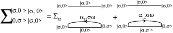
Figure 13: Graphical equation for the self-energy $\Sigma^{|\sigma,0\rangle|\sigma,0\rangle}_{|0,\sigma\rangle|\sigma,0\rangle}$.

$$\Sigma^{|\sigma,0\rangle|\sigma,0\rangle}_{|0,\sigma\rangle|\sigma,0\rangle}=\sum_{\alpha}\left\{P^{-,\sigma}_{\alpha_{12}}({\varepsilon_{1\sigma}})-i\pi\gamma^{-,\sigma}_{\alpha_{12}}(\varepsilon_{1\sigma})\right.$$

$$+\left.P^{+,\sigma}_{\alpha_{12}}({\varepsilon_{2\sigma}+U_{0}})+i\pi\gamma^{+,\sigma}_{\alpha_{12}}(\varepsilon_{2\sigma}+U_{0})\right\}\,,$$ (16)

with

$$P^{\pm,\sigma}_{\alpha_{ij}}({x})=\pm\frac{\Gamma_{\alpha ij}^{\sigma}}{2\pi}\left[{\rm Re}\Psi\left(\frac{1}{2}+i\frac{x-\mu_{\alpha}}{2\pi k_{B}T}\right)-\log\left({\frac{D}{2\pi k_{B}T}}\right)\right],$$ (17)

$$\gamma^{\pm,\sigma}_{\alpha_{ij}}(x)=\frac{\Gamma_{\alpha ij}^{\sigma}}{2\pi}f^{\pm}\left(x-\mu_{\alpha}\right),$$ (18)

where $f^{+}(x)$ stands for Fermi-Dirac distribution, $f^{-}(x)=1-f^{+}(x)$, and $\Psi(x)$ denotes the digamma function. Here, $D$ is the cut-off parameter which can be identified with on-level Coulomb repulsion $U$. It is worth to note that the self-energies do not depend on the cut-off parameter because the terms depending on $D$ cancel in pairs, see Eqs. (15) and (A).

References

- (1) W. G. van der Wiel, S. De Franceschi, J. M. Elzerman, T. Fujisawa, S. Tarucha, and L. P. Kouwenhoven, Rev. Mod. Phys. 75, 1 (2002).
- (2) D. Loss and D. P. DiVincenzo, Phys. Rev. A 57, 120 (1998).
- (3) R. Hanson and G. Burkard, Phys. Rev. Lett. 98, 050502 (2007).
- (4) K. Ono, D. G. Austing, Y. Tokura, and S. Tarucha, Science 297, 1313 (2002).
- (5) M. R. Gräber, W. A. Coish, C. Hoffmann, M. Weiss, J. Furer, S. Oberholzer, D. Loss, and C. Schönenberger, Phys. Rev. B 74, 075427 (2006).
- (6) D. T. McClure, L. DiCarlo, Y. Zhang, H.-A. Engel, C. M. Marcus, M. P. Hanson, and A. C. Gossard, Phys. Rev. Lett. 98, 056801 (2007).
- (7) V. N. Golovach and D. Loss, Phys. Rev. B 69, 245327 (2004).
- (8) E. Cota, R. Aguado, and G. Platero, Phys. Rev. Lett. 94, 107202 (2005).
- (9) J. Aghassi, A. Thielmann, M. H. Hettler, and G. Schön, Phys. Rev. B 73, 195323 (2006).
- (10) B. Wunsch, M. Braun, J. König, and D. Pfannkuche, Phys. Rev. B 72, 205319 (2005).
- (11) J. Fransson and M. Rasander, Phys. Rev. B 73, 205333 (2006).
- (12) S. Maekawa and T. Shinjo, Spin Dependent Transport in Magnetic Nanostructures (Taylor & Francis, New York, 2002).
- (13) I. Zutic, J. Fabian, and S. Das Sarma, Rev. Mod. Phys. 76, 323 (2004).
- (14) S. Maekawa, Concepts in Spin Electronics (Oxford University Press, 2006).
- (15) P. Trocha and J. Barnaś, Phys. Rev. B 76, 165432 (2007).
- (16) P. Trocha and J. Barnaś, (to appear in J. of Nanosci. and Nanotechnol.).
- (17) R. Hornberger, S. Koller, G. Begemann, A. Donarini, and M. Grifoni, Phys. Rev. B 77, 245313 (2008).
- (18) I. Weymann, Phys. Rev. B 75, 195339 (2007); Phys. Rev. B 78, 045310 (2008).
- (19) P. Trocha and J. Barnaś, Phys. Status Solidi B 244, 2553 (2007).
- (20) W. Rudziński and J. Barnaś, Phys. Rev. B 64, 085318 (2001).
- (21) M. Braun, J. König, and J. Martinek, Phys. Rev. B 70, 195345 (2004).
- (22) A. Cottet, W. Belzig, and C. Bruder, Phys. Rev. Lett. 92, 206801 (2004).
- (23) I. Weymann, J. König, J. Martinek, J. Barnaś, and G. Schön, Phys. Rev. B 72, 115334 (2005).
- (24) J. Martinek, Y. Utsumi, H. Imamura, J. Barnaś, S. Maekawa, J. König, and G. Schön, Phys. Rev. Lett. 91, 127203 (2003); M.-S. Choi, D. Sanchez, and R. Lopez, Phys. Rev. Lett. 92, 056601 (2004).
- (25) J. Barnaś and I. Weymann, J. Phys.: Condens. Matter 20, 423202 (2008).
- (26) S. Sahoo, T. Kontos, J. Furer, C. Hoffmann, M. Gräber, A. Cottet, and C. Schönenberger, Nat. Phys. 1, 99 (2005).
- (27) A. N. Pasupathy, R. C. Bialczak, J. Martinek, J. E. Grose, L. A. K. Donev, P. L. McEuen, and D. C. Ralph, Science 306, 86 (2004).
- (28) A. Bernand-Mantel, P. Seneor, N. Lidgi, M. Munoz, V. Cros, S. Fusil, K. Bouzehouane, C. Deranlot, A. Vaures, F. Petroff, and A. Fert, Appl. Phys. Lett. 89, 062502 (2006).
- (29) K. Hamaya, S. Masubuchi, M. Kawamura, T. Machida, M. Jung, K. Shibata, K. Hirakawa, T. Taniyama, S. Ishida, and Y. Arakawa, Appl. Phys. Lett. 90, 053108 (2007).
- (30) K. Hamaya, M. Kitabatake, K. Shibata, M. Jung, M. Kawamura, K. Hirakawa, T. Machida, T. Taniyama, S. Ishida, and Y. Arakawa, Appl. Phys. Lett. 91, 022107 (2007); Appl. Phys. Lett. 91, 232105 (2007).
- (31) K. Hamaya, M. Kitabatake, K. Shibata, M. Jung, M. Kawamura, S. Ishida, T. Taniyama, K. Hirakawa, Y. Arakawa, and T. Machida, Phys. Rev. B 77, 081302(R) (2008).
- (32) H. Yang, S.-H. Yang, and S. S. P. Parkin, Nano Lett. 8, 340 (2008).
- (33) K. Hamaya, M. Kitabatake, K. Shibata, M. Jung, S. Ishida, T. Taniyama, K. Hirakawa, Y. Arakawa, and T. Machida, Phys. Rev. Lett. 102, 236806 (2009).
- (34) H. Schoeller and G. Schön, Phys. Rev. B 50, 18436 (1994); J. König, J. Schmid, H. Schoeller, and G. Schön, Phys. Rev. B 54, 16820 (1996).
- (35) T. Kubo, Y. Tokura, T. Hatano, and S. Tarucha, Phys. Rev. B 74, 205310 (2006).
- (36) M. Julliere, Phys. Lett. A 54, 225 (1975).
- (37) J. Barnaś and A. Fert, Phys. Rev. Lett. 80, 1058 (1998); S. Takahashi and S. Maekawa, Phys. Rev. Lett. 80, 1758 (1998).
- (38) R. J. Soulen, Jr., J. M. Byers, M. S. Osofsky, B. Nadgorny, T. Ambrose, S. F. Cheng, P. R. Broussard, C. T. Tanaka, J. Nowak, J. S. Moodera, A. Barry, and J. M. D. Coey, Science 282, 85 (1998).
- (39) I. Weymann and J. Barnaś, J. Phys.: Condens. Matter 19, 096208 (2007).