CLOSED-ORBIT THEORY FOR SPATIAL DENSITY OSCILLATIONS

Abstract

We briefly review a recently developed semiclassical theory[1] for quantum oscillations in the spatial (particle and kinetic energy) densities of finite fermion systems and present some examples of its results. We then discuss the inclusion of correlations (finite temperatures, pairing correlations) in the semiclassical theory.

1 Introduction

We have recently proposed[1] a semiclassical theory for quantum oscillations in the local particle densities and kinetic-energy densities of a system of $N$ fermions in a local potential in $D$ dimensions, described by the stationary Schrödinger equation

$$\left\{-{\hbar^{2}\over 2m}\nabla^{2}+V({\bf r})\right\}\phi_{n}({\bf r})=E_{n}\,\phi_{n}({\bf r})\,.$$ (1)

The potential $V({\bf r})$ can be considered to represent the self-consistent mean field of an interacting system of fermions obtained in density functional theory (DFT).[2] The single-particle wavefunctions $\phi_{n}({\bf r})$ then are the Kohn-Sham orbitals[3] and $\rho({\bf r})$ in (2) is the (ideally exact) ground-state particle density of the interacting system.[4]

Ordering the spectrum $\{E_{n}\}$ and choosing the energy scale such that $0<E_{1}\leq E_{2}\leq\dots\leq E_{n}\leq\dots$, we fill the lowest levels up to the Fermi energy $\lambda$ and define the particle density by

$$\rho({\bf r})\;:=\;2\!\!\sum_{E_{n}\leq\lambda}\!\!|\phi_{n}({\bf r})|^{2},\qquad\int\rho({\bf r})\,{\rm d}^{D}r=N\,.$$ (2)

The factor 2 accounts for the spin degeneracy (the number $N$ is assumed to be even). Further degeneracies, which may arise for systems in $D>1$ dimensions, will not be spelled out bout included in the summations over $n$. For the kinetic-energy density, we consider two different definitions

$$\tau({\bf r})\;:=\;-\frac{\hbar^{2}}{2m}\;2\!\!\sum_{E_{n}\leq\lambda}\!\!\phi_{n}^{*}({\bf r})\nabla^{2}\phi_{n}({\bf r})\,,\qquad\tau_{1}({\bf r})\;:=\;\frac{\hbar^{2}}{2m}\;2\!\!\sum_{E_{n}\leq\lambda}\!\!|\nabla\phi_{n}({\bf r})|^{2},$$ (3)

which upon integration both yield the exact total kinetic energy.

The density of states $g(E)$ of the system (1) is given by

$$g(E)=\sum_{n}\delta(E-E_{n})\,,\qquad N=N(\lambda)=2\!\int_{0}^{\lambda}{\rm d}E\,g(E)\,.$$ (4)

Separating its smooth and oscillatory parts by defining

$$g(E):={\widetilde{g}}(E)+\delta g(E)\,,$$ (5)

the smooth part ${\widetilde{g}}(E)$ is given by the extended Thomas-Fermi (ETF) theory (see chapter 4.4.3 of Ref.[5]), while the the oscillating part $\delta g(E)$ can be described, to leading order in $\hbar$, by the semiclassical trace formula[6, 7]

$$\delta g(E)\simeq\sum_{\text{PO}}{\cal A}_{\text{PO}}(E)\cos\left[\frac{1}{\hbar}\,S_{\text{PO}}(E)-\frac{\pi}{2}\,\sigma_{\text{PO}}\right].$$ (6)

The sum here is over all periodic orbits (POs) of the corresponding classical system described by the Hamilton function $H({\bf q},{\bf p})={\bf p}^{2}\!/2m+V({\bf q})$. $S_{\text{PO}}(E)$ is the action integral along the periodic orbit:

$$S_{\text{PO}}(E)=\oint_{\text{PO}}{\bf p}(E,{\bf q})\cdot{\rm d}{\bf q}\,,$$ (7)

with the classical momentum given by ${\bf p}(E,{\bf r})=(\dot{{\bf r}}/|{\dot{\bf r}}|)\sqrt{2m[E-V({\bf r})]}$. For systems in which all orbits are isolated in phase space, explicit expressions for the amplitudes ${\cal A}_{\text{PO}}(E)$, which depend on the stabilities of the orbits, and for the Maslov indices $\sigma_{\text{PO}}$ have been given by Gutzwiller.[6] For systems with continuous symmetries and for integrable systems, alternative expressions for the amplitudes and Maslov indices have been derived by many authors; they may be found in Ref.[5]

Separating smooth and oscillating terms of the spatial densities

$$\rho({\bf r}):={\widetilde{\rho}}({\bf r})+\delta\rho({\bf r})\,,\quad\tau({\bf r}):={\widetilde{\tau}}({\bf r})+\delta\tau({\bf r})\,,\quad\tau_{1}({\bf r}):={\widetilde{\tau}}_{1}({\bf r})+\delta\tau_{1}({\bf r})\,,$$ (8)

the smooth parts are given by the ETF theory. For their oscillating parts we have obtained[1] the following semiclassical expressions, valid again to leading order in $\hbar$:

$$\delta\rho({\bf r}) \simeq \sum_{\gamma}{\cal A}_{\gamma}(\widetilde{\lambda},{\bf r})\,\cos\left[\Phi_{\gamma}(\widetilde{\lambda},{\bf r})\right],$$ (9)

$$\delta\tau({\bf r}) \simeq \frac{{\bf p}^{2}(\widetilde{\lambda},{\bf r})}{2m}\,\sum_{\gamma}{\cal A}_{\gamma}(\widetilde{\lambda},{\bf r})\,\cos\left[\Phi_{\gamma}(\widetilde{\lambda},{\bf r})\right],$$ (10)

$$\delta\tau_{1}({\bf r}) \simeq \frac{{\bf p}^{2}(\widetilde{\lambda},{\bf r})}{2m}\,\sum_{\gamma}{\cal A}_{\gamma}(\widetilde{\lambda},{\bf r})\,Q_{\gamma}(\widetilde{\lambda},{\bf r})\,\cos\left[\Phi_{\gamma}(\widetilde{\lambda},{\bf r})\right].$$ (11)

The sum here is over all closed orbits $\gamma$ starting and ending in the point ${\bf r}$, and

$$\Phi_{\gamma}(\widetilde{\lambda},{\bf r})=\frac{1}{\hbar}S_{\gamma}(\widetilde{\lambda},{\bf r})-\frac{\pi}{2}\,\mu_{\gamma}-\frac{\pi}{4}\,(D+1)\,.$$ (12)

The action function $S_{\gamma}(\widetilde{\lambda},{\bf r})=S_{\gamma}(\widetilde{\lambda},{\bf r},{\bf r}^{\prime}={\bf r})$ is gained from the general open action integral for an orbit starting at ${\bf r}$ and ending at ${\bf r}^{\prime}$ at fixed energy $E=\widetilde{\lambda}$

$$S_{\gamma}(\widetilde{\lambda},{\bf r},{\bf r}^{\prime})=\int_{{\bf r}}^{{\bf r}^{\prime}}{\bf p}(\widetilde{\lambda},{\bf q})\cdot{\rm d}\,{\bf q}\,,$$ (13)

and $\mu_{\gamma}$ is the Morse index that counts the number of conjugate points along the orbit.[6, 7] For the functions ${\cal A}_{\gamma}(\widetilde{\lambda},{\bf r})$ and $Q_{\gamma}(\widetilde{\lambda},{\bf r})$ we refer to our articles.[1, 8, 9] The quantity $\widetilde{\lambda}$ is the Fermi energy of the smooth (ETF) system, defined by

$$\lambda=\widetilde{\lambda}+\delta\lambda\,,\qquad N=2\int_{0}^{\widetilde{\lambda}}{\rm d}E\,{\widetilde{g}}(E)\,.$$ (14)

Since for POs the action integral $S_{\text{PO}}(\widetilde{\lambda})$ is independent of ${\bf r}$, they do not yield any oscillating phases in the above expressions; their contributions vary only smoothly with ${\bf r}$ through ${\cal A}_{\rm PO}(\widetilde{\lambda},{\bf r})$ and $Q_{\rm PO}(\widetilde{\lambda},{\bf r})$. The leading contributions to the density oscillations come from the non-periodic orbits (NPOs). For one-dimensional systems ($D$=1) it has, in fact, been shown[1, 8] that the contributions of the POs are completely absorbed by the smooth (TF) densities. In higher-dimensional systems, the POs must be included in (9) - (11) in connection with symmetry breaking at ${\bf r}=0$ for spherical systems, and with bifurcations at finite distances $|{\bf r}|>0$ in general, as demonstrated explicitly for the two-dimensional circular billiard.[9]

2 Selected results

In this section we give some selected results of our semiclassical theory. We first present a very general result that may have interesting consequences for DFT. From (9), (10) one finds directly – without knowledge of the orbits $\gamma$ – the relation

$$\delta\tau({\bf r})\simeq[\widetilde{\lambda}-V({\bf r})]\,\delta\rho({\bf r})\,,$$ (15)

which we call the (differential) local virial theorem (LVT) because it relates the potential and kinetic-energy densities locally at any given point ${\bf r}$. The relation (15) was derived[10] for isotropic harmonic oscillators in arbitrary dimensions from their quantum-mechanical densities in the asymptotic limit $N\to\infty$. In our semiclassical theory it is obtained for arbitrary potentials. Since no assumption about the potential or the nature of the closed orbits $\gamma$ must be made to derive the LVT (15), it holds for arbitrary (integrable or non-integrable) systems in arbitrary dimensions with a local potential $V({\bf r})$, and hence also for interacting fermions in the mean-field approximation given by the DFT. We recall, however, that (15) is not expected to be valid close to the classical turning points where the semiclassical expressions (9) - (11) diverge and must be regularized by appropriate uniform approximations.[8, 9]

A direct consequence of the LVT in (15) is the following relation:

$$\tau({\bf r})\;\simeq\;\tau_{\text{TF}}[\rho({\bf r})]\,.$$ (16)

Hereby $\tau_{\text{TF}}[\rho_{\text{TF}}({\bf r})]=\tau_{\text{TF}}({\bf r})$ is the exact functional relation between the TF kinetic-energy and particle densities. Eq. (16) states that this TF functional (without gradient corrections!) holds approximately, for arbitrary local potentials $V({\bf r})$, also between the exact quantum-mechanical densities $\tau({\bf r})$ and $\rho({\bf r})$ including their quantum oscillations. [It was shown in Ref.[8] to be exact up to first order in $\delta\rho({\bf r})$.]

In Fig. 1 we test (16) explicitly for the coupled two-dimensional quartic oscillator

$$V(x,y)=\frac{1}{2}(x^{4}+y^{4})-\kappa\,x^{2}y^{2}\,,$$ (17)

whose classical dynamics is almost chaotic[11, 12] in the limits $\kappa=1$ and $\kappa\to-\infty$, but in practice also for $\kappa=0.6$ (see, e.g., Ref.[13]).

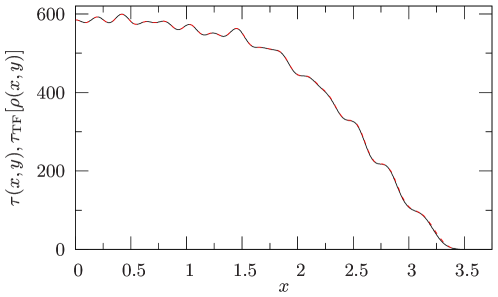
Figure 1: TF relation (16) for the potential (17) with $\kappa=0.6$ (units: $\hbar=m=1$) with $N=632$. Cuts along the diagonal $x=y$. The solid line is the l.h.s., and the dashed line is the r.h.s. of (16).

We find an excellent agreement over the whole region. That the TF kinetic-energy functional holds also for the oscillating exact densities to a surprising degree has been noted long ago,[14] but not understood until now. Similarly good numerical results are obtained also for the LVT (15), except very close to the classical turning points, for many systems[8, 9] with not too small particle numbers $N$.

Figure 2: Particle density in the 2-dimensional circular billiard with various particle numbers $N$ (units: $\hbar^{2}\!/2m=R=1$). Dotted lines: quantum results, solid lines: semiclassical results.[9]

Next we present some results for the particle densities. Figure 2 shows $\rho(r)$ for four values of the number of $N$ particles bound in the two-dimensional circular billiard. The dotted line is the quantum result (2), and the solid line the converged semiclassical result (9), complemented by uniform approximations at the critical points as explained in detail in Ref.[9]  Similar results are obtained also for the kinetic-energy densities, and for other types of potentials.[1, 8]

It should be emphasized that, due to a factor $1/T_{\gamma}(\widetilde{\lambda},{\bf r})$ in the semiclassical amplitudes ${\cal A}_{\gamma}(\widetilde{\lambda},{\bf r})$ in (9) - (11), the sums over the orbits $\gamma$ converge much faster than in the trace formula (6) for the level density.

Note the Friedel oscillations in Fig. 2 near the surface ($r=R$), which are characteristic of a fermionic system near a steep boundary. In our semiclassical theory, the Friedel oscillations are caused by the shortest orbit with one reflection from the boundary (in Refs.[1, 8] called the primitive “+” orbit). Its regularized contribution to the particle density of a spherical billiard in $D$ dimensions is[8]

$$\delta\rho_{+}(r)=-\rho_{\text{TF}}^{(D)}\,2^{\nu}\Gamma(\nu+1)\left(\frac{R}{r}\right)^{\!\nu-1/2}\frac{J_{\nu}(z)}{z^{\nu}}\,,$$ (18)

where $\rho_{\text{TF}}^{(D)}$ is the TF density, $\nu=D/2$,  $z=2\,(R-r)\,p_{\lambda}/\hbar$, and $p_{\lambda}=(2m\widetilde{\lambda})^{1/2}$ is the smooth Fermi momentum. Integrating (18) over the whole space, we obtain

$$\delta N_{+}=\int{\rm d}^{D}r\,\delta\rho_{+}(r)=-\frac{1}{2\pi^{D/2}\hbar^{D-1}}\,\frac{\Gamma(D/2)}{\Gamma(D)}\,p_{\lambda}^{D-1}\,{\cal S}_{D}\,,$$ (19)

where ${\cal S}_{D}=2\pi^{D/2}R^{D-1}\!/\Gamma(D/2)$ is the hypersurface of the $D$-dimensional sphere. It is interesting to note (see also Ref.[15]) that (19) corresponds precisely to the surface term in the Weyl expansion[16] of the particle number $N(\widetilde{\lambda})$ which varies smoothly with the Fermi energy (the volume term being given by the TF theory).

3 Inclusion of finite temperatures in the semiclassical theory

In the following we outline how to include finite temperatures in the semiclassical formalism. Extensions of semiclassical trace formulae to finite temperatures have been used long ago in the context of nuclear physics[17] and more recently in mesoscopic physics.[18] We shall present here a derivation by means of a suitable folding function, which has proved useful also in the corresponding microscopic theories[19] and allows for a straightforward generalization to include other types of correlations.

For a grand-canonical ensemble of fermions embedded in a heat bath with fixed temperature, the variational energy is the so-called grand potential $\Omega$ defined by

$$\Omega=\langle{\hat{H}}\rangle-TS-\lambda\langle{\hat{N}}\rangle\,,$$ (20)

where ${\hat{H}}$ and ${\hat{N}}$ are the Hamilton and particle number operators, respectively, $T$ is the temperature in energy units (i.e., we put the Boltzmann constant $k_{\text{B}}$ equal to unity), $S$ is the entropy, and $\lambda$ the chemical potential. Note that both energy and particle number are conserved only on the average. For non-interacting particles, we can write the Helmholtz free energy $F$ as

$$F=\langle{\hat{H}}\rangle-TS=2\sum_{n}E_{n}\nu_{n}-TS\,.$$ (21)

Here $\nu_{n}$ are the Fermi occupation numbers

$$\nu_{n}=\frac{1}{1+\exp{\left(\frac{E_{n}-\lambda}{T}\right)}}\,,$$ (22)

and the entropy $S$ is given by

$$S=-2\sum_{n}\,[\nu_{n}\log\nu_{n}+(1-\nu_{n})\log(1-\nu_{n})]\,.$$ (23)

The chemical potential $\lambda$ is determined by fixing the average particle number

$$N=\langle{\hat{N}}\rangle=2\sum_{n}\nu_{n}\,.$$ (24)

Note that all sums in (21) – (24) and below run over the complete (infinite) spectrum of the Hamiltonian ${\hat{H}}$.

It has been shown[19] that the above quantities $F$, $N$ and $S$ can be expressed in terms of a convoluted finite-temperature level density $g_{T}(E)$ defined by a convolution of the “cold” ($T=0$) density of states (4)

$$g_{T}(E):=\int_{-\infty}^{\infty}g(E^{\prime})\,f_{T}(E-E^{\prime})\,{\rm d}E^{\prime}=\sum_{n}f_{T}(E-E_{n})\,,$$ (25)

whereby the folding function $f_{T}(E)$ is given as

$$f_{T}(E)=\frac{1}{4T\,{\rm cosh}^{2}(E/2T)}\,.$$ (26)

The free energy then is given by

$$F=2\int_{-\infty}^{\lambda}E\,g_{T}(E)\,{\rm d}E\,,$$ (27)

and the average particle number by

$$N=2\int_{-\infty}^{\lambda}g_{T}(E)\,{\rm d}E\,.$$ (28)

To show that the integral (27) gives the correct free energy (21), including the “heat energy” $-TS$, requires some algebraic manipulations. From $F$, the entropy $S$ can always be gained by the canonical relation

$$S=-\frac{\partial F}{\partial T}\,.$$ (29)

The same convolution can now be applied also to the semiclassical trace formula (6) for the oscillating part of the density of states which we re-write as

$$\delta g(E)\simeq\text{Re}\sum_{\text{PO}}{\cal A}_{\text{PO}}(E)\,e^{i\Phi_{\text{PO}}(E)}$$ (30)

with the phase

$$\Phi_{\rm PO}(E)=\frac{1}{\hbar}\,S_{\text{PO}}(E)-\frac{\pi}{2}\,\sigma_{\text{PO}}\,.$$ (31)

The oscillating part $\delta g_{T}(E)$ of the finite-temperature level density is obtained by the convolution of (30) with the function $f_{T}(E)$ as in (25). In the spirit of the stationary-phase approximation, we take the slowly varying amplitude ${\cal A}_{\text{PO}}(E)$ outside of the integration and approximate the action in the phase by

$$S_{\text{PO}}(E^{\prime})\simeq S_{\text{PO}}(E)+(E^{\prime}-E)\,T_{\text{PO}}(E)\,,$$ (32)

so that the result becomes a modified trace formula

$$\delta g_{T}(E)\simeq\text{Re}\sum_{\text{PO}}{\cal A}_{\text{PO}}(E)\,{\tilde{f}}_{T}[{\cal T}_{\text{PO}}(E)]\,e^{i\Phi_{\text{PO}}(E)},$$ (33)

where

$${\cal T}_{\text{PO}}(E)=T_{\text{PO}}(E)/\hbar\,$$ (34)

and the temperature modulation factor ${\tilde{f}}_{T}$ is given by the Fourier transform of the convolution function $f_{T}$:

$${\tilde{f}}_{T}({\cal T})=\int_{-\infty}^{\infty}f_{T}(\omega)\,e^{i{\cal T}\omega}\,{\rm d}\omega\,.$$ (35)

The Fourier transform of the function (26) is known[20] and yields

$${\tilde{f}}_{T}({\cal T})=\frac{\pi T{\cal T}}{{\rm sinh}(\pi T{\cal T})}\,.$$ (36)

The “hot” trace formulae (33) with the modulation factor (36) has previously been obtained in Refs.[17, 18] The trace formula for the oscillating part of the free energy then becomes[5, 17] to leading order in $\hbar$

$$\delta F\simeq\text{Re}\sum_{\text{PO}}{\cal A}_{\text{PO}}(\widetilde{\lambda})\,\left(\frac{\hbar}{T_{\text{PO}}(\widetilde{\lambda})}\right)^{\!2}{\tilde{f}}_{T}[{\cal T}_{\text{PO}}(\widetilde{\lambda})]\,e^{i\Phi_{\text{PO}}(\widetilde{\lambda})}.$$ (37)

For the spatial densities we can proceed exactly in the same way. For the particle density, e.g., the microscopic expression (2) is replaced by

$$\rho_{T}({\bf r})=2\sum_{n}|\phi_{n}({\bf r})|^{2}\nu_{n}\,,$$ (38)

where the sum again runs over the complete spectrum. Starting from the semiclassical expression (9) for $\delta\rho(r)$ at $T=0$, we rewrite it as

$$\delta\rho_{0}(\widetilde{\lambda},{\bf r})\simeq\text{Re}\sum_{\gamma}{\cal A}_{\gamma}(\widetilde{\lambda},{\bf r})\,e^{i\Phi_{\gamma}(\widetilde{\lambda},{\bf r})},$$ (39)

where $\Phi_{\gamma}(\widetilde{\lambda},{\bf r})$ is the phase (12). The finite-$T$ expression is given by the convolution integral

$$\delta\rho_{T}(\widetilde{\lambda},{\bf r})\simeq\int_{-\infty}^{\widetilde{\lambda}}\delta\rho_{0}(\widetilde{\lambda}-E,{\bf r})f_{T}(E)\,{\rm d}E\,.$$ (40)

Expanding the phase under the integral as above, we arrive at

$$\delta\rho_{T}(\widetilde{\lambda},{\bf r})\simeq\text{Re}\sum_{\gamma}{\cal A}_{\gamma}(\widetilde{\lambda},{\bf r})\,{\tilde{f}}_{T}[{\cal T}_{\gamma}(\widetilde{\lambda},{\bf r})]\,e^{i\Phi_{\gamma}(\widetilde{\lambda},{\bf r})}\,,$$ (41)

where ${\cal T}_{\gamma}(\widetilde{\lambda},{\bf r})=T_{\gamma}(\widetilde{\lambda},{\bf r})/\hbar$. The corresponding expressions for the temperature-dependent kinetic-energy densities are obvious.

For the smooth parts of the densities, we recall that the ETF theory at $T>0$ is well known (see, e.g. Ref.[21], where expressions up to 4-th order in $\hbar$ are given, and the literature quoted therein).

Other types of correlations can be included in the semiclassical theory in the same way, as soon as a suitable folding function $f_{\text{corr}}(E)$ – corresponding to $f_{T}(E)$ in (26) – and its Fourier transform are known. One example is given by the pairing correlations discussed in the following section.

4 Inclusion of pairing correlations in the BCS approximation

A self-consistent microscopic approach to include pairing correlations is given by the Hartree-Fock-Bogolyubov (HFB) approach; we refer to an extended article[19] for a recapitulation of this theory and the relevant literature. In the simplified BCS approach with constant paring gap $\Delta$, the total energy of a system is written as

$$E_{\text{BCS}}=\sum_{n}E_{n}v_{n}^{2}-\Delta\sum_{n}u_{n}v_{n}\,,$$ (42)

where the sum goes over the complete spectrum (including all degeneracies) and the occupation numbers $u_{n}$ and $v_{n}$ are given by

$$v_{n} = \frac{1}{\sqrt{2}}\left[1+\frac{(\lambda-E_{n})}{{\cal E}_{n}}\right]^{1/2},$$

$$u_{n} = \sqrt{1-v_{n}^{2}}\,.$$ (43)

Hereby ${\cal E}_{n}$ is the so-called quasiparticle energy

$${\cal E}_{n}(\lambda)={{}_{+}\!}\sqrt{(\lambda-E_{n})^{2}+\Delta^{2}}\,.$$ (44)

It was shown[19] that the BCS energy (42) is correctly given, including the pair condensation energy

$$E_{p}=-\,\Delta\sum_{n}u_{n}v_{n}\,,$$ (45)

by the convolution integral

$$E_{\text{BCS}}=\int_{-\infty}^{\lambda}E\,f_{\Delta}(E)\,{\rm d}E\,,$$ (46)

where the folding function $f_{\Delta}(E)$ is defined as

$$f_{\Delta}(E):=\frac{\Delta^{2}}{2\left[E^{2}+\Delta^{2}\right]^{3/2}}.$$ (47)

The Fermi energy $\lambda$ in all above expressions is fixed by the average particle number:

$$N=\int_{-\infty}^{\lambda}g_{\Delta}(E)\,{\rm d}E=\sum_{n}v_{n}^{2}\,.$$ (48)

The “paired” level density $g_{\Delta}(E)$ is given by

$$g_{\Delta}(E)=\sum_{n}\frac{\Delta^{2}}{2\left[{\cal E}_{n}(E)\right]^{3}}.$$ (49)

The Fourier transform of $f_{\Delta}(E)$ is found[20] to be

$${\widetilde{f}}_{\Delta}({\cal T})=\Delta{\cal T}K_{1}(\Delta{\cal T})\,,$$ (50)

where $K_{1}(z)$ is a modified Bessel function.[22] Hence, replacing ${\widetilde{f}}_{T}$ in (33) by ${\widetilde{f}}_{\Delta}$, the semiclassical trace formula for the oscillating part of the paired level density becomes

$$\delta g_{\Delta}(E)\simeq\text{Re}\sum_{\text{PO}}{\cal A}_{\text{PO}}(E)\,{\tilde{f}}_{\Delta}[{\cal T}_{\text{PO}}(E)]\,e^{i\Phi_{\text{PO}}(E)}.$$ (51)

The trace formula for the oscillating part of the total BCS energy becomes, analogously to (37),

$$\delta E_{\rm BCS}\simeq\text{Re}\sum_{\text{PO}}{\cal A}_{\text{PO}}(\widetilde{\lambda})\,\left(\frac{\hbar}{T_{\text{PO}}(\widetilde{\lambda})}\right)^{\!2}{\tilde{f}}_{\Delta}[{\cal T}_{\text{PO}}(\widetilde{\lambda})]\,e^{i\Phi_{\text{PO}}(\widetilde{\lambda})}.$$ (52)

That for the pair condensation energy, using $E_{p}=\Delta\,\partial E_{\rm BCS}/\partial\Delta$ and exploiting a recurrence relation for the Bessel functions,[22] becomes

$$\delta E_{p}\simeq\Delta^{2}\,\text{Re}\sum_{\text{PO}}{\cal A}_{\text{PO}}(\widetilde{\lambda})\,K_{0}[{\cal T}_{\text{PO}}(\widetilde{\lambda})]\,e^{i\Phi_{\text{PO}}(\widetilde{\lambda})}.$$ (53)

A similar result has recently been obtained in Ref.[23]

For the spatial densities we can, in principle, proceed as above. The pair-correlated particle density is quantum-mechanically given by[19]

$$\rho_{\Delta}({\bf r})=\sum_{n}|\phi_{n}({\bf r})|^{2}v_{n}^{2}\,.$$ (54)

The semiclassical expression of its oscillating part becomes, similarly as above,

$$\delta\rho_{\Delta}(\widetilde{\lambda},{\bf r})\simeq\text{Re}\sum_{\gamma}{\cal A}_{\gamma}(\widetilde{\lambda},{\bf r})\,{\tilde{f}}_{\Delta}[{\cal T}_{\gamma}(\widetilde{\lambda})]\,e^{i\Phi_{\gamma}(\widetilde{\lambda},{\bf r})}\,.$$ (55)

Corresponding results hold for the pair-correlated kinetic-energy densities.

This is, however, not the end of the story. If one wants to express the pair-condensation energy (45) as a space integral, one requires an anomalous density matrix $\kappa({\bf r},{\bf r}^{\prime})$, defined by[19]

$$\kappa({\bf r},{\bf r}^{\prime})=\sum_{n}\phi_{n}({\bf r})\phi_{\bar{n}}({\bf r}^{\prime})\,,$$ (56)

where ${\bar{n}}$ refers to the time-reversed state of $n$. The semiclassical evaluation of this anomalous density matrix is the object of our ongoing research.

References

• [1] J. Roccia and M. Brack, Phys. Rev. Lett. 100, 200408 (2008).
• [2] M.R. Dreizler and E.K.U. Gross: Density Functional Theory  (Springer-Verlag, Berlin, 1990).
• [3] W. Kohn and L.J. Sham, Phys. Rev. A 137, 1697 (1965); ibidem 140, 1133 (1965).
• [4] P. Hohenberg and W. Kohn, Phys. Rev. 136, B864 (1964).
• [5] M. Brack and R. K. Bhaduri: Semiclassical Physics, Frontiers in Physics, Vol. 96 (revised edition: Westview Press, Boulder, 2003).
• [6] M.C. Gutzwiller, J. Math. Phys. 12, 343 (1971).
• [7] M.C. Gutzwiller: Chaos in classical and quantum mechanics (Springer-Verlag, New York, 1990).
• [8] J. Roccia, M. Brack, A. Koch, and M.V.N. Murthy, Preprint Regensburg/Chennai (2009); arXiv:0903.2172v3 [math-phys]
• [9] M. Brack and J. Roccia, J. Phys. A 42, 355210 (2009).
• [10] M. Brack and M.V.N. Murthy, J. Phys. A 36, 1111 (2003).
• [11] O. Bohigas, S. Tomsovic, and D. Ullmo, Phys. Rep. 223, 43 (1993).
• [12] A.B. Eriksson and P. Dahlqvist, Phys. Rev. E 47, 1002 (1993).
• [13] M. Gutiérrez, M. Brack, K. Richter, and A. Sugita, J. Phys. A 40, 1525 (2007).
• [14] M. Brack in: From nuclei to bose condensates, Festschrift for the 65th birthday of Rajat K. Bhaduri (Regensburg and Chennai, 2000), p. 35;
results quoted also in M. Brack and B. van Zyl, Phys. Rev. Lett. 86, 1574 (2001).
• [15] W.-M. Zheng, Phys. Rev. E 60, 2845 (1999).
• [16] see, e.g., H.P. Baltes and E.R. Hilf: Spectra of Finite Systems (B.-I. Wissenschaftsverlag, Mannheim, 1976).
• [17] V.M. Kolomietz, A.G. Magner, and V.M. Strutinsky, Yad. Fiz. 29, 1478 (1979);
A.G. Magner, V.M. Kolomietz, and V.M. Strutinsky, Izvestiya Akad. Nauk SSSR, Ser. Fiz. 43, 142 (1979).
• [18] K. Richter, D. Ullmo, R. Jalabert, Phys. Rep. 276, 1 (1996).
• [19] M. Brack and P. Quentin, Nucl. Phys. A 361, 35 (1981).
• [20] H. Bateman: Tables of integral transforms, Vol. 1 (McGraw-Hill, New York, 1954).
• [21] J. Bartel, M. Brack, and M. Durand, Nucl. Phys. A 445, 263 (1985).
• [22] M. Abramowitz and I.A. Stegun: Handbook of Mathematical Functions (Dover Publications, 9th printing, New York, 1970).
• [23] H. Olofsson, S. Åberg, and P. Leboeuf, Phys. Rev. Lett. 100, 037005 (2008);
see also S. Åberg, H. Olofsson, and P. Leboeuf, AIP Conf. Proc. 995, 173 (2008).