Geometric curvatures of plane symmetry black hole

Abstract

In this paper, we study the properties and thermodynamic stability of the plane symmetry black hole from the viewpoint of geometry. Weinhold metric and Ruppeiner metric are obtained, respectively. The Weinhold curvature gives phase transition points, which correspond to the first-order phase transition only at $N=1$, where $N$ is a parameter in the plane symmetry black hole. While the Ruppeiner one shows first-order phase transition points for arbitrary $N\neq 1$. Both of which give no any information about the second-order phase transition. Considering the Legendre invariant proposed by Quevedo et. al., we obtain a unified geometry metric, which gives a correctly the behavior of the thermodynamic interactions and phase transitions. The geometry is also found to be curved and the scalar curvature goes to negative infinity at the Davies’ phase transition points when the logarithmic correction is included.

I Introduction

Several decades ago, the original works of Bekenstein and Hawking showed that the black hole is indeed a thermodynamics system Bekenstein1973prd ; Hawking1975cmp . It was also found that the black hole satisfies four laws of the elementary thermodynamics with regarding the surface gravity and the outer horizon area as its temperature and entropy, respectively Hawking1973cmp . Although, it is widely believed that a black hole is a thermodynamic system, the statistical origin of the black hole entropy is still one of the most fascinating and controversial subjects today.

The investigation of thermodynamic properties of black holes is also a fascinating subject. Much of work had been carried out on the stability and phase transitions of black holes. It is generally thought that the local stability of a black hole is mainly determined by its heat capacity. Negative heat capacity usually gives a thermodynamically unstable system and the positive one implies a local stable one. The points, where the heat capacity diverges, are usually consistent with the Davies’ points, where the second-order phase transition takes place Davies1977 .

The properties of a thermodynamic system can also be studied with the ideas of geometry. Weinhold Weinhold1975jcp firstly introduced the geometrical concept into the thermodynamics. He suggested that a Riemannian metric can be defined as the second derivatives of internal energy $U$ with respect to the entropy and other extensive quantities of a thermodynamic system. However, it seems that the Weinhold geometry has not much physical meanings. Few years later, Ruppeiner Ruppeiner1979pra introduced another metric, which is analogous to the Weinhold one. The thermodynamic potential of the Ruppeiner geometry is the entropy $S$ of the thermodynamic system rather than the internal energy $U$. In fact, the two metrics are conformally related to each other

$$ds^{2}_{R}=\frac{1}{T}ds^{2}_{W},$$ (1)

with the temperature $T$ as the conformal factor. The Ruppeiner geometry had been used to study the ideal gas and the van der Waals gas. It was shown that the curvature vanishes for the ideal gas whereas, for the van der Waals gas, the curvature is non-zero and diverges only at those points, the phase transitions take place(for details see the review paper Ruppeiner1995rmp ). The black hole, as a thermodynamics system, has been extensively investigated. The Weinhold geometry and the Ruppeiner geometry were obtained for various black holes and black branes Davies1977 ; Weinhold1975jcp ; Ruppeiner1979pra ; Ruppeiner1995rmp ; Ferrara1997npb ; cai1999prd ; Aman2003grg ; Johnston2003app ; Arcioni2005prd ; Shen2007ijmpa ; Aman2006grg ; Aman2006prd ; Mirza2006jhep ; Aman2008eps ; Aman2008 ; Medved2008mpla ; Myung2008plb ; Gergely2008 ; Wei2009prd ; Biswas2009 ; Sarkar2008jhep ; Bellucci2008 ; Aman2007jpcs ; Ruppeiner2008prd ; Vacaru1999 . In particular, it was found that the Ruppeiner geometry carries the information of phase structure of a thermodynamic system. In general, its curvature is singular at the points, where the phase transition takes place. However, for the rotating Banados-Teitelboim-Zanelli (BTZ) and Reissner-Nordstr$\ddot{o}$m (RN) black holes, the cases are quite different. The Ruppeiner geometry gives a vanished curvature, which means there exists no thermodynamic interactions and no phase transition points. But the two kinds of black hole do exist the phase transition points. For this contradiction, many researches has been carried out to explain it. The main focus is on the thermodynamic potential, which is generally believed to be the internal energy $U$ rather than the mass $M$ for simple. For the Reissner-Nordstr$\ddot{o}$m black hole, it was argued in Mirza2006jhep that, the thermodynamic curvature should be reproduced from the Kerr-Newmann anti-de sitter black hole with the angular momentum $J\rightarrow 0$ and cosmological constant $\Lambda\rightarrow 0$. Another explanation of the contradiction was presented by Queved et. al. few years ago Quevedo2007jmp ; Quevedo2008prc . They pointed out that the origin of the contradiction is that the Weinhold metric and Ruppeiner metric are not Legendre invariant. A Legendre invariant metric was introduced by them, which could reproduce correctly the behavior of the thermodynamic interactions and phase transitions for the BTZ and RN black holes Quevedo2009prd ; Quevedo2008grg and other black hole configurations and models Alvarez2008prd ; Quevedo2008jhep ; Quevedo2008 ; 2Quevedo2009prd .

Another interesting and important question of this field is how the geometry behaves when including the corrected term of the entropy. It is generally believed that, for a canonical ensemble, there exists a logarithmic corrected term to the entropy Huang1963 . Considering the correction term, the geometry structure was studied in Quevedo2009prd ; Sarkar2006jhep for the BTZ black hole. Especially, its Ruppeiner curvature will become non-zero when the logarithmic correction is included. The aim of this paper is to study the phase transitions and geometry structure of the plane symmetry black hole. Firstly, we study the thermodynamic stability of the plane symmetric black hole. It is shown that there always exist locally thermodynamically stable phases and unstable phases for the plane symmetric black hole due to suitable parameter regimes. Then, three different geometry structures are obtained. The Weinhold curvature gives phase transition points, which correspond to that of the first-order phase transition only at $N=1$. While the Ruppeiner one shows first-order phase transition points for arbitrary $N\neq 1$. Both of which give no any information about the second-order phase transition. Considering the Legendre invariant, we obtain a unified geometry metric, which gives a correct behavior of the thermodynamic interactions and phase transitions. It is found that the curvature constructed from the unified metric goes to negative infinity at the Davies’ points, where the second-order phase transition takes place. The geometry structure is also studied as the logarithmic correction is included. The result shows that the logarithmic correction term has no affect on the unified geometry depicts the phase transitions of the plane symmetric black hole. We also show that the absolute values of the charge $Q$ at the divergence points of the curvature $\mathcal{R}^{\prime}_{L}$ will decrease with the increase of the entropy corrected parameter $\gamma$ for large $S$.

The paper is organized as follows. In Sec. II, we first review some thermodynamic quantities of the plane symmetric black hole. The thermodynamic stability is also studied. In Sec. III, both the Weinhold and Ruppeiner geometry structures are obtained. However, they fail to give the information about the second-order phase transition points. For the reason, we give a detail analysis and obtain a new Legendre invariant metric structure which could give a well description of the thermodynamic interactions and phase transitions in Sec. IV. Including the logarithmic corrected term, the geometry structure is considered in Sec. V. Finally, the paper ends with a brief conclusion.

II Thermodynamic Quantities and Thermodynamic Stability of the Plane Symmetric Black Hole

In this section, we will present the thermodynamic quantities and other properties of the plane symmetric black hole. The thermodynamic stability of it is also discussed. The action depicting the plane symmetric black hole is given by

$$S=\frac{1}{16\pi}\int d^{4}x\sqrt{-g}\big{(}\mathcal{R}-2(\nabla\varphi)^{2}-2\Lambda e^{2b\varphi}-e^{-2a\varphi}F^{2}\big{)}.$$ (2)

where $\varphi$ is a dilaton field and $a$, $b$ are constants. The negative cosmological constant $\Lambda=-3\alpha^{2}$. Static plane symmetric black hole solutions in this theory were first given in Cai1996prd (some detail works for this black hole can also be found in Miranda2008jhep ; Zeng2009ctp ; Zeng2009IJTP ; Lemos2004prd )

$$ds^{2}=-f(r)dt^{2}+f^{-1}(r)dr^{2}+g(r)(dx^{2}+dy^{2}).$$ (3)

The metric functions are given by, respectively,

$$f(r) = -\frac{4\pi M}{N\alpha^{N}}r^{1-N}+\frac{6\alpha^{2}}{N(2N-1)}r^{N}+\frac{2Q^{2}}{N\alpha^{2N}}r^{-N},$$ (4)

$$g(r) = (r\alpha)^{N}.$$ (5)

where $N\in(\frac{1}{2},2)$. The parameters $M$ and $Q$ are the mass and charge of the black hole. The event horizon is located at $f(r_{h})=0$ and the radius $r_{h}$ satisfies

$$\frac{3\alpha^{2}}{2N-1}r_{h}^{2N}-\frac{2\pi M}{\alpha^{N}}r_{h}+\frac{Q^{2}}{\alpha^{2N}}=0.$$ (6)

In general, there exist two event horizons, the inner event horizon and the outer event horizon. Under the extreme case, the two horizon will merge into each other. Here, we have denoted $r_{h}$ as the radius of outer event horizon.

The surface area of the event horizon corresponds to unit $xoy$ plane Zeng2009IJTP

$$\mathcal{A}=(\alpha r_{h})^{2N}.$$ (7)

From Eq. (6), the mass can be expressed in the form

$$M=\frac{3\alpha^{N+2}}{2\pi(2N-1)}r_{h}^{2N-1}+\frac{Q^{2}}{2\pi\alpha^{N}}r_{h}^{-1}.$$ (8)

With the relation between area and entropy, i.e. $S=\frac{\mathcal{A}}{4}$, we can obtain

$$r_{h}=\frac{1}{\alpha}(4S)^{\frac{1}{2N}}.$$ (9)

Substituting Eq. (9) into (8), the mass can be obtained as a function of entropy $S$ and charge $Q$ in the form

$$M=\frac{3\alpha^{3-N}}{2\pi(2N-1)}(4S)^{\frac{2N-1}{2N}}+\frac{Q^{2}}{2\pi\alpha^{N-1}}(4S)^{-\frac{1}{2N}}.$$ (10)

From the energy conservation law of the black hole

$$dM=TdS+\phi dQ,$$ (11)

the relevant thermodynamic variables, the temperature and electric potential are obtained

$$T = \left(\frac{\partial M}{\partial S}\right)_{Q}=\frac{(12\alpha^{2}S-Q^{2})\alpha^{1-N}}{2^{2+\frac{1}{N}}\pi NS^{1+\frac{1}{2N}}},$$ (12)

$$\phi = \left(\frac{\partial M}{\partial Q}\right)_{S}=\frac{\alpha^{1-N}Q}{2^{\frac{1}{N}}\pi S^{\frac{1}{2N}}}.$$ (13)

For a given charge $Q$, the heat capacity has the expression

$$C_{Q}=-\frac{2NS(12\alpha^{2}S-Q^{2})}{12S\alpha^{2}-(1+2N)Q^{2}}\;,$$ (14)

with the zero-points and singular points

$$Q^{2} = 12\alpha^{2}S,\quad\quad\mbox{(zero-points)}$$ (15)

$$Q^{2} = \frac{12\alpha^{2}S}{2N+1},\quad\;\mbox{(singular points)}$$ (16)

respectively. The heat capacity $C_{Q}$ vanishes at $Q^{2}=12\alpha^{2}S$, which is considered to be the first-order phase transition points. It is generally believed that the Davies’ points where the second-order phase transition takes place correspond to the diverge points of heat capacity. So the heat capacity (14) may indicate that the second-order phase transition takes place at $Q^{2}=\frac{12\alpha^{2}S}{2N+1}$. The heat capacity also contains the information of the local stability of the black hole thermodynamics. The negative heat capacity always implies an unstable thermodynamics system and the positive one shows a stable system. Here, we would like to give a brief discussion about the local stability of the plane symmetric black hole. For $Q^{2}>12\alpha^{2}S$, the numerator of the heat capacity (14) is negative, while the denominator is positive, which gives a negative heat capacity. For $Q^{2}<\frac{12\alpha^{2}S}{2N+1}$, the numerator is positive, but the denominator turns to negative, which also shows a negative heat capacity. So, in both cases, the heat capacity $C_{Q}$ implies an unstable black hole thermodynamics. When $|Q|\in(2\sqrt{3}\alpha\sqrt{\frac{S}{2N+1}},2\sqrt{3}\alpha\sqrt{S})$, both the numerator and denominator are positive, which implies a stable black hole thermodynamics. The behavior of the heat capacity $C_{Q}$ can be directly found from Fig. 1. For Larger and smaller values of $|Q|$, the heat capacity $C_{Q}$ is negative. While in the middle zone, it is positive. In summary, we have found that there always exist locally thermodynamically stable phases and unstable phases for the plane symmetric black hole due to suitable parameter regimes.

Figure 1: The behavior of the heat capacity $C_{Q}$, with $N=1$, $\alpha=\frac{\sqrt{3}}{3}$ and $S=100$. $C_{Q}$ is singular at $Q=\pm 11.5470$ and vanishes at $Q=\pm 20$.

III Weinhold geometry and Ruppeiner geometry of the Plane Symmetric Black Hole

In this section, we would like to study the Weinhold geometry and Ruppeiner geometry of the plane symmetric black hole. In the first step, we will show the Weinhold geometry. Then, using the conformal relation, we could obtain the Ruppeiner geometry. The Weinhold geometry is charactered by the metric

$$ds_{W}^{2}=\frac{\partial^{2}M}{\partial S^{2}}dS^{2}+2\frac{\partial^{2}M}{\partial S\partial Q}dSdQ+\frac{\partial^{2}M}{\partial Q^{2}}dQ^{2},$$ (17)

where the index $W$ denotes the Weinhold geometry. Here, we have made the choice that the mass $M$ corresponds to the thermodynamic potential and with the extensive variables entropy $S$ and charge $Q$.

Using Eq. (10), the Weinhold metric can be obtained in the form

$$g_{W}=-\frac{\alpha^{1-N}}{2^{\frac{1}{N}}S^{\frac{1}{2N}}}\left(\begin{array}[]{cc}\frac{12\alpha^{2}S-(2N+1)Q^{2}}{8\pi N^{2}S^{2}}&\frac{Q}{2\pi NS}\\ \frac{Q}{2\pi NS}&-\frac{1}{\pi}\\ \end{array}\right).$$ (20)

Its determinant is $\det(g)=-\frac{\alpha^{2-2N}[12\alpha^{2}S-(2N-1)Q^{2}]}{2^{3+\frac{2}{N}}S^{2+\frac{1}{N}}\pi^{2}N^{2}}$. It can be seen that the determinant disappears as the heat capacity vanishes only at $N=1$. A simple calculation shows that the Christoffel symbols are

$$\Gamma^{S}_{SS} = -\frac{(2N+1)\big{[}12\alpha^{2}S-(4N-1)Q^{2}\big{]}}{4NS\big{[}12\alpha^{2}S-(2N-1)Q^{2}\big{]}},\quad\Gamma^{S}_{QS}=\Gamma^{S}_{SQ}=-\frac{2NQ}{12\alpha^{2}S-(2N-1)Q^{2}},$$

$$\Gamma^{S}_{QQ} = -\frac{2NS}{12\alpha^{2}S-(2N-1)Q^{2}},\quad\quad\quad\quad\quad\quad\Gamma^{Q}_{SS}=-\frac{(2N+1)Q^{3}}{4NS^{2}\big{[}12\alpha^{2}S-(2N-1)Q^{2}\big{]}},\quad$$ (21)

$$\Gamma^{Q}_{SQ} = \Gamma^{Q}_{QS}=-\frac{12\alpha^{2}S+(2N+1)Q^{2}}{4S\big{[}12N\alpha^{2}S-N(2N-1)Q^{2}\big{]}},\quad\Gamma^{Q}_{QQ}=\frac{Q}{12\alpha^{2}S-(2N-1)Q^{2}},\quad$$

where the Christoffel symbols is calculated with

$$\Gamma^{\lambda}_{\mu\nu} = \frac{1}{2}g^{\lambda\tau}(g_{\nu\tau,\mu}+g_{\mu\tau,\nu}-g_{\mu\nu,\tau}).$$ (22)

The Riemannian curvature tensor, Ricc curvature and scalar curvature are given, respectively

$$R^{\mu}_{\sigma\nu\tau}=\Gamma^{\mu}_{\sigma\nu,\tau}-\Gamma^{\mu}_{\sigma\tau,\nu}+\Gamma^{\mu}_{\lambda,\tau}\Gamma^{\lambda}_{\sigma,\nu}-\Gamma^{\mu}_{\lambda,\nu}\Gamma^{\lambda}_{\sigma,\tau},$$

$$R_{\mu\nu}=R^{\lambda}_{\mu\lambda\nu},$$ (23)

$$R=g^{\mu\nu}R_{\mu\nu}.$$

With Eq. (23), we get the scalar curvature

$$\mathcal{R}_{W}=-\frac{24\;2^{\frac{1}{N}}N\pi S^{1+\frac{1}{2N}}\alpha^{1+N}}{\big{[}12\alpha^{2}S-(2N-1)Q^{2}\big{]}^{2}}.$$ (24)

This curvature is always negative for any values of charge $Q$ and positive entropy $S$. It diverges at $Q^{2}=\frac{12\alpha^{2}S}{2N+1}$, which consists with the first-order transition points (15) reproduced from the capacity $C_{Q}$ only at $N=1$. Its behavior can be seen in Fig. 2. However, it implies no information about the second-order phase transition. So, it is natural to ask how the Ruppeiner curvature behaves. Could it gives the proper phase transition points?

Figure 2: The negative Weinhold curvature $\mathcal{R}_{w}$ vs. the charge Q with $N=1$, $\alpha=\frac{\sqrt{3}}{3}$ and $S=100$. The divergence points are at $Q=\pm 20$.

With that question, we now turn to the Ruppeiner geometry of the plane symmetric black hole. Recalling the conformal relation between the Ruppeiner geometry and the Weinhold geometry, we obtain the Ruppeiner metric

$$g_{R}=\frac{1}{T}g_{W}=\left(\begin{array}[]{cc}-\frac{12\alpha^{2}S-(2N+1)Q^{2}}{2NS(12\alpha^{2}S-Q^{2})}&-\frac{2Q}{12\alpha^{2}S-Q^{2}}\\ -\frac{2Q}{12\alpha^{2}S-Q^{2}}&-\frac{4NS}{12\alpha^{2}S-Q^{2}}\\ \end{array}\right),$$ (27)

where the index $R$ denotes the Ruppeiner geometry. After some calculations, we obtain the Ruppeiner curvature

$$\mathcal{R}_{R}=-\frac{12\alpha^{2}Q^{2}(N-1)\big{[}36S\alpha^{2}-(4N-1)Q^{2}\big{]}}{(12\alpha^{2}S-Q^{2})\big{[}12S\alpha^{2}-(2N-1)Q^{2}\big{]}^{2}}.$$ (28)

It is obvious that the curvature will be zero at $N=1$. The vanished thermodynamic curvature $\mathcal{R}_{R}$ implies that there exists no phase transition points and no thermodynamic interactions appear. So, the Ruppeiner curvature is not proper to describe the phase transitions of the plane symmetric black hole at $N=1$. The divergence of the Ruppeiner curvature is at $Q^{2}=\frac{12\alpha^{2}S}{2N-1}$ and $Q^{2}=12\alpha^{2}S$, which can be seen from the Fig. (3). The points $Q^{2}=12\alpha^{2}S$ consist with the zero-points (15) of heat capacity $C_{Q}$. This means that the Ruppeiner curvature always implies the first-order phase transition points. Like the Weinhold curvature, the Ruppeiner curvature also implies no any information about the second-order phase transition.

Figure 3: The negative Ruppeiner curvature $\mathcal{R}_{R}$ vs. the charge Q with $N=\frac{3}{2}$, $\alpha=\frac{\sqrt{3}}{3}$ and $S=100$. The divergence points are at $Q=\pm 20,\pm 14.1421$.

IV Unified geometry of the Plane Symmetric Black Hole

In the previous section, we show that the Weinhold curvature implies the first-order phase transition points only at $N=1$, while the Ruppeiner curvature implies the first-order phase transition points expect $N=1$. Both of the geometry structures fail to give the second-order phase transition points of the plane symmetric black hole. Quevedo et. al. pointed out the failure of the two geometries to describe the second-order phase transition points is that they are not Legendre invariant, which makes them inappropriate to describe the geometry of thermodynamic systems Quevedo2008grg . Considering the Legendre invariant, a unified geometry was presented in Alvarez2008prd , where the metric structure can give a well description of various types of black hole thermodynamics. So, in this section, we would like to discuss the unified geometry of the plane symmetric black hole and we want to know whether it works.

The unified geometry metric can be expressed as

$$ds^{2}_{L} = \bigg{(}S\frac{\partial M}{\partial S}+Q\frac{\partial M}{\partial Q}\bigg{)}\left(\begin{array}[]{cc}-\frac{\partial^{2}M}{\partial S^{2}}&0\\ 0&\frac{\partial^{2}M}{\partial Q^{2}}\\ \end{array}\right)\left(\begin{array}[]{c}dS^{2}\\ dQ^{2}\\ \end{array}\right)$$ (34)

$$= \frac{\alpha^{2-2N}\big{[}12\alpha^{2}S-(2N+1)Q^{2}\big{]}\big{[}12\alpha^{2}S+(4N-1)Q^{2}\big{]}}{2^{5+\frac{2}{N}}\pi^{2}N^{3}S^{2+\frac{1}{N}}}dS^{2}$$

$$+\frac{\alpha^{2-2N}(12\alpha^{2}S+(4N-1)Q^{2})}{2^{\frac{2(N+1)}{N}}\pi^{2}NS^{\frac{1}{N}}}dQ^{2}.$$

The index $L$ denotes the curvature reproduced from the Legendre invariant metric. This diagonal metric reproduces the thermodynamic curvature $\mathcal{R}_{L}$, which turns out to be non-zero and the scalar curvature is

$$\mathcal{R}_{L} = \frac{192\;4^{\frac{1}{N}}\pi^{2}\alpha^{2N}NS^{1+\frac{1}{N}}}{\big{[}12\alpha^{2}S-(2N+1)Q^{2}\big{]}^{2}\big{[}12\alpha^{2}S+(4N-1)Q^{2}\big{]}^{3}}$$ (35)

$$\cdot\bigg{\{}(4N-1)Q^{2}\big{[}(N(4N^{2}-6N-3)-1)Q^{2}$$

$$~{}-12((N-5)N-2)\alpha^{2}S\big{]}+144(N-1)^{2}\alpha^{4}S^{2}\bigg{\}}.$$

The thermodynamic curvature vanishes at $Q^{2}=12S\alpha^{2}$ when $N=1$, which is just the points of the first-order phase transition. It is shown that the diverge points are at $Q^{2}=\frac{12\alpha^{2}S}{2N+1}$, which implies that there exists second-order phase transitions at that points. This result exactly consists with that of the heat capacity (14). The detail behavior of $\mathcal{R}_{L}$ can be found in Fig. 4, where the singularities are just the divergence points of the heat capacity $C_{Q}$. Now, we can see that the thermodynamic curvature $\mathcal{R}_{L}$ reproduced from the Legendre invariant metric (34) could give an exact description of the second-order phase transitions of a thermodynamics system. Beside this, we also expect that this unified geometry description may give more information about a thermodynamics system.

Figure 4: The negative unified geometric curvature $\mathcal{R}_{L}$ vs. the charge Q with $N=1$, $\alpha=\frac{\sqrt{3}}{3}$ and $S=100$. The divergence points are at $Q=\pm 11.5470$, which are consistent with the divergence points of the heat capacity $C_{Q}$. The positive curvature region is at $|Q|\geq 20$ and it is not shown in this figure.

V Inclusion of logarithmic correction

In this section, we will discuss the unified geometry of the plane symmetric black hole when the logarithmic corrected term is included. For general, we suppose that the correct-entropy formula is of the form

$$S^{\prime}=S-\gamma\ln S.$$ (36)

The parameter $\gamma$ is a constant. In fact, the origin of the logarithmic correction term can be accounted by the uncertainty principle or the tunneling method.

With Eq. (36), the heat capacity (14) is modified to

$$C^{\prime}_{Q}=\frac{2NS(S-\gamma)(S-\gamma\ln S)(12S\alpha^{2}-Q^{2}-12\alpha^{2}\gamma\ln S)}{A_{2}Q^{2}-A_{1}},$$ (37)

with

$$A_{1} = 12\alpha^{2}(S-\gamma{\ln}S)\big{[}\big{(}1+2N\ln{S}\big{)}\gamma^{2}-2(N+1)S{\gamma}+S^{2}\big{]},$$ (38)

$$A_{2} = \big{[}2N(1+\ln S)+1\big{]}\gamma^{2}-2(3N+1)S\gamma+(2N+1)S^{2}.$$ (39)

The singular points of the heat capacity are determined by $A_{2}Q^{2}-A_{1}=0$ and are given by

$$Q^{2}=\frac{A_{1}}{A_{2}}.$$ (40)

If $\gamma=0$, the singular points of the heat capacity will become Eq. (14). Following the Sec. IV, we obtain the curvature $\mathcal{R}^{\prime}_{L}$:

$$\mathcal{R}^{\prime}_{L}=\frac{h(S,Q,N,\gamma)}{K^{3}(A_{2}Q^{2}-A_{1})^{2}},$$ (41)

where $K=[4N(S-\gamma\ln S)+\gamma-S]Q^{2}+12\alpha^{2}(S-\gamma)(S-\gamma\ln S)$, and $h(S,Q,N,\gamma)$ is a complex function and we do not write it here. It is found that the divergence points for the heat capacity $C^{\prime}_{Q}$ and the curvature $\mathcal{R}^{\prime}_{L}$ consist with each other, which means the curvature give proper points, where second-order phase transitions take place. So, it is easy to summarized that the logarithmic correction term does not affect the unified geometry to depict the plane symmetry black hole’s phase transitions.

Now, we would like to discuss how the geometry behaved as the parameter $\gamma$ takes different values. For simplicity, we turn back to the case $N=1$. The Legendre invariant metric for this case is

$$g_{L}=\left(\begin{array}[]{cc}-\frac{BC}{128\pi^{2}S^{2}(S-\gamma\ln S)^{4}}&0\\ 0&\frac{B}{16\pi^{2}S^{2}(S-\gamma\ln S)^{2}}\\ \end{array}\right),$$ (44)

where $B=K|_{N=1}$ and $C=(A_{2}Q^{2}-A_{1})|_{N=1}$ After some tedious calculations, we can obtain the curvature. The numerator of the curvature is a cumbersome expression and can not be written in a compact form. While the denominator of it is proportional to the determinant of the metric (44) and is given by

$$D=B^{3}\cdot C^{2}.$$ (45)

Fixing the parameters $\alpha$ and entropy $S$, the characteristic behavior of the curvature is depicted in Fig. 5, where the parameter $\gamma$ is set to $\frac{1}{2}$, $\frac{5}{6}$ and $\frac{3}{2}$, respectively. The values of the charge $Q$ at the divergence points of the curvature $\mathcal{R}^{\prime}_{L}$ are given as

$$Q=\pm 2\sqrt{3}\alpha\sqrt{\frac{{(S-\gamma\ln S)\big{[}\big{(}1+2\ln{S}\big{)}\gamma^{2}-4S{\gamma}+S^{2}\big{]}}}{{\big{[}2(1+\ln S)+1\big{]}\gamma^{2}-8S\gamma+3S^{2}}}}.$$ (46)

When $\Delta=3-2\ln S\geq 0$, there are three points of $\gamma$ for the vanished charge $Q$:

$$\gamma_{1}=\frac{S}{\ln S},\;\;\gamma_{\pm}=\frac{2\pm\sqrt{3-2\ln S}}{1+2\ln S}S.$$ (47)

In general, we consider $S\gg 1$, which leads to $\Delta<0$. So, the vanished charge $Q$ is only at $\gamma=\gamma_{1}$. From Fig. 6, it is easy to conclude that the absolute values of the charge $Q$ at the divergence points of the curvature $\mathcal{R}^{\prime}_{L}$ will decrease with the increase of the parameter $\gamma$ for large $S$.

Figure 5: The negative unified geometric curvature $\mathcal{R}_{L}$ vs. the charge Q, including the logarithmic correction. The values of $\alpha$ and the entropy $S$ are the same in Fig. 4. The parameter $\gamma$ is set to $\frac{1}{2}$(left), $\frac{5}{6}$(middle) and $\frac{3}{2}$(right), respectively. The divergence points are at $Q=\pm 11.3756$, $\pm 11.2613$ and $\pm 11.0326$.

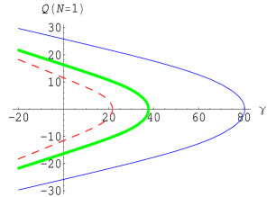
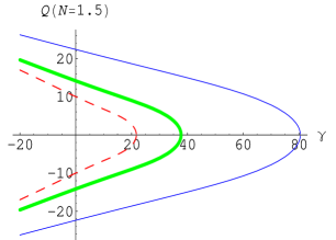
Figure 6: The value of charge $Q$ at divergence points of the curvature $\mathcal{R}^{\prime}_{L}$ vs. parameter $\gamma$. The parameter $\alpha$ is set to $\frac{\sqrt{3}}{3}$. The entropy is set to $S=100$ for red dashed lines, $S=200$ for green thick lines and $S=500$ for blue thin lines.

VI Conclusion

In this paper, we study the phase transitions and geometry structure of the plane symmetry black hole. The local thermodynamic stability of it is also discussed through the heat capacity $C_{Q}$. It is shown that there always exist locally thermodynamically stable phases and unstable phases for plane symmetric black hole due to suitable parameter regimes. The Weinhold geometry and the Ruppeiner geometry are obtained. The Weinhold curvature gives phase transition points, which correspond to that of the first-order phase transition only at $N=1$. While the Ruppeiner one shows first-order phase transition points for arbitrary $N\neq 1$. Both of which give no any information about the second-order phase transition. Quevedo et. al. first pointed out that the two geometry metrics are not Legendre invariant and they introduced a Legendre invariant metric, which can give a well description of various types black hole thermodynamics. Considering the Legendre invariant, we obtain a unified geometry metric, which gives a correct behavior of the thermodynamic interaction and second-order phase transition. Including the logarithmic corrected term, we study the geometry structure of the plane symmetry black hole. The result show that the logarithmic correction term does not affect the unified geometry to depict the phase transitions of it. We also obtain the result that, for large $S$, the absolute values of the charge $Q$ at the divergence points of the curvature $\mathcal{R}^{\prime}_{L}$ will decrease with the increase of the parameter $\gamma$. In this paper, we show that the unified geometry description gives a well description of the second-order phase transitions of the plane symmetry black hole. We also expect that this unified geometry description may give more information about a thermodynamic system.

References

- (1) J. D. Bekenstein, Phys. Rev. D 7 (1973) 2333.
- (2) S. W. Hawking, Commun. Math. Phys. 43 (1975) 199.
- (3) J. M. Bardeen, B. Carter and S. W. Hawking, Commun. Math. Phys. 31 (1973) 161.
- (4) P. C. W. Davies, Proc. Roy. Soc. Lond. A 353 (1977) 499; P. C. W. Davies, Rep. Prog. Phys. 41 (1977) 1313; P. C. W. Davies, Class. Quant. Grav. 6 (1989) 1909.
- (5) F. Weinhold, J. Chem. Phys. 63 (1975) 2479.
- (6) G. Ruppeiner, Phys. Rev. A 20 (1979) 1608.
- (7) G. Ruppeiner, Rev. Mod. Phys. 67 (1995) 605; 68 (1996) 313(E).
- (8) S. Ferrara, G. W. Gibbons and R. Kallosh, Nucl. Phys. B 500 (1997) 75, arXiv:hep-th/9702103.
- (9) R. G. Cai and J. H. Cho, Phys. Rev. D 60 (1999) 067502, arXiv:hep-th/9803261.
- (10) J. Aman, I. Bengtsson and N. Pidokrajt, Gen. Rel. Grav. 35 (2003) 1733, arXiv:gr-qc/0304015.
- (11) D. A. Johnston, W. Janke and R. Kenna, Acta Phys. Polon. B 34 (2003) 4923, arXiv:cond-mat/0308316.
- (12) G. Arcioni and E. L. Tellechea, Phys. Rev. D 72 (2005) 104021, arXiv:hep-th/0412118.
- (13) J. Y. Shen, R. G. Cai, B. Wang and R. K. Su, Int. J. Mod. Phys. A 22 (2007) 11, arXiv:gr-qc/0512035.
- (14) J. E. Aman, I. Bengtsson and N. Pidokrajt, Gen. Rel. Grav. 38 (2006) 1305, arXiv:gr-qc/0601119.
- (15) J. E. Aman, N. Pidokrajt, Phys. Rev. D 73 (2006) 024017, arXiv:hep-th/0510139.
- (16) B. Mirza and M. Zamaninasab, JHEP 0706 (2007) 059, arXiv:0706.3450[hep-th].
- (17) J. E. Aman, N. Pidokrajt and J. Ward, EAS Publ. Ser. 30 (2008) 279, arXiv:0711.2201[hep-th].
- (18) Jan E. Aman and N. Pidokrajt, Ruppeiner Geometry of Black Hole Thermodynamics, arXiv:0801.0016[gr-qc].
- (19) A. J. M. Medved, Mod. Phys. Lett. A 23 (2008) 2149, arXiv:0801.3497[gr-qc].
- (20) Y. S. Myung, Y. W. Kim and Y. J. Park, Phys. Lett. B 663 (2008) 342, arXiv:0802.2152[hep-th].
- (21) L. A. Gergely, N. Pidokrajt and S. Winitzki, Thermodynamics of tidal charged black holes, arXiv:0811.1548[gr-qc].
- (22) Y. H. Wei, Phys. Rev. D 80 (2009) 024029.
- (23) R. Biswas and S. Chakraborty, The geometry of the higher dimensional black hole thermodynamics in Einstein-Gauss-Bonnet theory, arXiv:0905.1776[gr-qc]; R. Biswas and S. Chakraborty, Black holes in the Einstein -Gauss-Bonnet theory and the geometry of their thermodynamics-II, arXiv:0905.1801[gr-qc].
- (24) T. Sarkar, G. Sengupta and B. N. Tiwari, JHEP 0810 (2008) 076, arXiv:0806.3513[hep-th].
- (25) S. Bellucci and B. N. Tiwari, On the Microscopic Perspective of Black Branes Thermodynamic Geometry, arXiv:0808.3921[hep-th].
- (26) J. E. Aman, J. Bedford, D. Grumiller, N. Pidokrajt and J. Ward, J. Phys. Conf. Ser. 66 (2007) 012007, arXiv:gr-qc/0611119.
- (27) G. Ruppeiner, Phys. Rev. D 78 (2008) 024016, arXiv:0802.1326[gr-qc].
- (28) S. I. Vacaru, Thermodynamic Geometry and Locally Anisotropic Black Holes, arXiv:gr-qc/9905053.
- (29) H. Quevedo, J. Math. Phys. 48 (2007) 013506, arXiv:physics/0604164[physics.chem-ph].
- (30) H. Quevedo and A. Vazquez, AIPConf. Proc. 977 (2008)165, arXiv:0712.0868[math-ph].
- (31) H. Quevedo and A. Sanchez, Phys. Rev. D 79 (2009) 024012, arXiv:0811.2524[gr-qc].
- (32) H. Quevedo, Gen. Rel. Grav. 40 (2008) 971, arXiv:0704.3102[gr-qc].
- (33) J. L. Alvarez, H. Quevedo and A. Sanchez, Phys. Rev. D 77 (2008) 084004, arXiv:0801.2279[gr-qc].
- (34) H. Quevedo and A. Sanchez, JHEP 0809 (2008) 034, arXiv:0805.3003[hep-th].
- (35) H. Quevedo, A. Sanchez and A. Vazquez, Invariant geometry of the ideal gas, arXiv:0811.0222[math-ph].
- (36) H. Quevedo and A. Sanchez, Phys. Rev. D 79 (2009) 087504, arXiv:0902.4488[gr-qc].
- (37) K. Huang, Statistical Mechanics, Publishers John Wiley, 1963; L. D. Landau and E. M. Lifshitz, Statistical Physics, Publishers Pergamon, 1969.
- (38) T. Sarkar, G. Sengupta and B. N. Tiwari, JHEP 0611 (2006) 015, arXiv:hep-th/0606084.
- (39) R. G. Cai and Y. Z. Zhang, Phys. Rev. D 54 (1996) 4891, arXiv:gr-qc/9609065.
- (40) A. S. Miranda, J. Morgan and V. T. Zanchin, JHEP 0811 (2008) 030, arXiv:0809.0297[hep-th]; A. S. Miranda and V. T. Zanchin, Phys.Rev. D 73 (2006) 064034, arXiv:gr-qc/0510066.
- (41) X. X. Zeng, Y. W. Han and Y. S. Zheng, Commun. Theor. Phys. 51 (2009) 187.
- (42) R. Zhao, L. C. Zhang and Y. Q. Wu, Int. J. Theor. Phys. 46 (2007) 3128.
- (43) J. P. Lemos and F. S. Lobo, Phys. Rev. D 69 104007 (2004), arXiv:gr-qc/0402099.