Anisotropic transport in quantum wires embedded in (110) plane

Abstract

We investigate theoretically the effects of the Coulomb interaction and spin-orbit interactions (SOIs) on the anisotropic transport property of semiconductor quantum wires embedded in (110) plane. The anisotropy of the dc conductivity can be enhanced significantly by the Coulomb interaction for infinite-long quantum wires. But it is smeared out in quantum wires with finite length, while the ac conductivity still shows anisotropic behavior, from which one can detect and distinguish the strengths of the Rashba SOI and Dresselhaus SOI.

All-electrical manipulation of spin degree of freedom is one of the central issues and the ultimate goal of spintronics field. The spin-orbit interaction (SOI) provides us an efficient way to control electron spin electrically and therefore has attracted tremendous interest from the view of point both the potential application in all-electrical controlled spintronic devices and fundamental physics.¹ The SOI is manifest of the relativistic effect and caused by the broken of spatial inversion symmetry.² The spatial inversion symmetry can be broken by the structure inversion symmstry (SIA) and bulk crystal inversion symmetry, named Rashba SOI (RSOI) and Dresselhaus SOI (DSOI), respectively.${}^{3\text{,}4}$ In thin quantum wells, the strength of the DSOI is comparable to that of the RSOI since the strength of the DSOI depends significantly on the thickness of quantum wells. The interplay between the RSOI and the DSOI leads to interesting phenomena, e.g., the anisotropic photogalvanic effect⁵, the persistent spin helix⁶, and anisotropic transport property of quantum wire^7,8.

Changing the crystallographic planes can have a significant effect on the interplay between RSOI and DSOI, which is a consequence of the fact that the DSOI depends sensitively on the crystallographic planes electrons are moving in. It is highly desirable to study how the crystallographic plane affects the transport property, which is interesting and important for potential applications of semiconductor spintronic devices. Very recently, the anisotropic behavior of transport property in semiconductor quantum wire was proposed to detect the relative strength between the RSOI and DSOI in a quasi-one-dimensional (Q1D) semiconductor quantum wire system.⁷ But the effect of the Coulomb interaction on the transport property is not addressed. Since the Coulomb interaction becomes very important for Q1D systems where electrons are strongly correlated, the conventional Fermi liquid theory breaks down. We will address this issue in this Letter based on the Luttinger liquid (LL) theory⁹. The LL is of fundamental importance because it is one of very few strongly correlated non-Fermi liquid systems that can be solved analytically. The RSOI would lead to the mixing between the spin and charge excitations.^10-13 The LL behavior was demonstrated experimentally in many Q1D system, e.g., narrow quantum wire formed in semiconductor heterostructures¹⁴, carbon nanotube¹⁵, graphene nanoribbon¹⁶, as well as the edge states of the fractional Quantum Hall liquid¹⁷.

In this Letter, we investigate theoretically the Coulomb interaction on the anisotropic transport properties in semiconductor quantum wires at (110) crystallographic plane in the presence of the RSOI and DSOI. We find that, in contrary to the non-interacting electron gas, the anisotropy of the dc transport property is smeared out for a quantum wire with finite length. The ac conductivity still depends sensitively on the crystallographic direction, which provides us a possible way to detect the strengths of the RSOI and DSOI in Q1D semiconductor quantum wire.

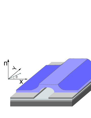
Figure 1: (color online) Schematic diagram of semiconductor quantum wire which can be fabricated along the crystallographic direction $\theta$ with respect to $[100]$ axis in the crystallographic planes $(110)$.

For a clean Q1D quantum wire embedded in (110) plane (see Fig. 1), the Hamiltonian of the noninteracting electrons reads⁸

$$H_{0}=\frac{\hbar^{2}k_{x}^{2}}{2m^{\ast}}+V(r)-\alpha\sigma_{y}k_{x}-\frac{1}{2}\beta sin\theta\sigma_{z}k_{x},$$ (1)

where $\theta$ is the angle between the orientation of the quantum wire and the [100] axis, $m^{\ast}$ is the electron effective mass, $\sigma_{i}$ ($i$=$x,y,z$) are the Pauli matrices, $\alpha$ and $\beta$ are the strengths of the RSOI and DSOI, respectively. Assuming $\delta v\ll v_{F}$ ($v_{F}$ is the bare Fermi velocity of right and left moving noninteracting electrons), the linearized noninteracting electron Hamiltonian of the quantum wire with both RSOI and DSOI is given by^10,13 $H_{0}=-i\hbar\int\sum_{\gamma,s}v_{\gamma}^{s}\psi_{\gamma s}^{+}\partial_{x}\psi_{\gamma s}dx$, where the operators $\psi_{\gamma s}$ $(\gamma=-1(L),1(R);s=-1(\downarrow),1(\uparrow))$ annihilate spin-down $(\downarrow)$ or spin-up $(\uparrow)$ electrons near the left (L) and right $(R)$ Fermi points, respectively. $v_{\gamma}^{s}=\gamma v_{F}-s\delta v$ are the four different Fermi velocities, where $\delta v$=$\sqrt{\alpha^{2}+\beta^{2}sin^{2}\theta/4}/\hbar$. Note that the RSOI and DSOI split the spin subbands and make the electron Fermi velocities become different for different directions of motion. The total Hamiltonian of the system is $H=H_{0}+H_{int}$, where $H_{int}\!\!=\!\!\frac{1}{2}\int\int dxdy\psi_{\gamma s}^{\dagger}(x)\psi_{\gamma^{{}^{\prime}}\!s^{{}^{\prime}}}^{\dagger}(y)V\!\!_{\gamma\gamma^{{}^{\prime}}}(x-y)\psi_{\gamma^{{}^{\prime}}\!s^{{}^{\prime}}}(y)\psi_{\gamma s}(x)$. The Umklapp scattering process is neglected because the Fermi energy in quantum wires formed in semiconductor heterostructure is far from the half-filled case. And the electron-electron backscattering can be negligible for a sufficiently long interacting region.¹⁰ Using the bosonization technique¹⁸, the Hamiltonian becomes

$$H = \frac{\hbar}{2}\int dx\Big{[}\frac{v_{\rho}}{K_{\rho}}(\partial_{x}\vartheta_{\rho})^{2}+v_{\rho}K_{\rho}\Big{(}\frac{\Pi_{\rho}}{\hbar}\Big{)}^{2}\Big{]}$$ (2)

$$+ \frac{\hbar}{2}\int dx\Big{[}\frac{v_{\sigma}}{K_{\sigma}}(\partial_{x}\vartheta_{\sigma})^{2}+v_{\sigma}K_{\sigma}\Big{(}\frac{\Pi_{\sigma}}{\hbar}\Big{)}^{2}\Big{]}$$

$$+ \hbar\delta v\int dx\Big{[}\Big{(}\frac{\Pi_{\sigma}}{\hbar}\Big{)}(\partial_{x}\vartheta_{\rho})+\Big{(}\frac{\Pi_{\rho}}{\hbar}\Big{)}(\partial_{x}\vartheta_{\sigma})\Big{]},$$

where $\vartheta_{\rho}$ and $\vartheta_{\sigma}$ are the phase fields for the charge and spin degrees of freedom, respectively, and $\Pi_{\rho}$ and $\Pi_{\sigma}$ are the corresponding conjugate momenta. $v_{\rho,\sigma}$ are the propagation velocities of the charge and spin collective modes of the decoupled model ($\delta v=0$). In the following, we consider only pointlike density-density interactions. $v_{\rho,\sigma}$=$v_{F}/K_{\rho,\sigma}$ ¹⁸, and the parameter $K_{\rho/\sigma}$ is defined as $1/K_{\rho/\sigma}^{2}$=$1\pm g$, where $g$=2$V(q$=0)/$\hbar\pi v_{F}$ with $V(q$=0) is the electron-electron interaction potential.

We consider an interacting Q1D quantum wire under a time-dependent electric field $E(x,t)$ along the wire, e.g., a microwave radiation. $H_{ac}=-\sqrt{\frac{2}{\pi}}e\int dxE(x,t)\vartheta_{\rho}(x,t)$ describes the interaction between electron and radiation field in the quantum wire.¹⁹ The total Hamiltonian becomes $H=H_{0}+H_{int}+H_{ac}$. Using the equation of motion and the linear response theory, we obtain the nonlocal charge conductivity

$$\sigma_{\rho}(x,\omega) = \frac{2e^{2}}{h}\Bigg{[}\frac{(u_{1}^{2}-v_{\sigma}^{2}+\delta v^{2})}{(u_{1}^{2}-u_{2}^{2})}\frac{v_{F}}{u_{1}}e^{i\frac{\omega}{u_{1}}|x|}$$ (3)

$$- \frac{(u_{2}^{2}-v_{\sigma}^{2}+\delta v^{2})}{(u_{1}^{2}-u_{2}^{2})}\frac{v_{F}}{u_{2}}e^{i\frac{\omega}{u_{2}}|x|}\Bigg{]},$$

where

$$u_{1,2}^{2}\!\!=\frac{v_{\rho}^{2}+v_{\sigma}^{2}}{2}+\delta v^{2}\pm\!\sqrt{\Big{(}\frac{v_{\rho}^{2}\!-\!v_{\sigma}^{2}}{2}\Big{)}^{2}\!\!+2\delta v^{2}(v_{\rho}^{2}\!+v_{\sigma}^{2})},$$ (4)

where $u_{1,2}$ are the propagation velocities of coupled collective modes that depend on the crystallographic orientation $\theta$. Notice that the SOIs couple the spin and charge excitations in the absence of the SOIs.

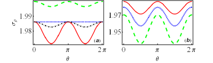
Figure 2: (color online) The dc conductivity (in units of $K_{\rho}e^{2}/h$) as a function of the angle $\theta$. (a)with fixed $g$=0.4 where solid red line is for $\alpha$=0.2 and $\beta$=0.4, the dot-dashed black line for $\alpha$=0.2 and $\beta$=0.2, the dashed green line for $\alpha$=0 and $\beta$=0.2, and the dotted blue line for $\alpha$=0.2 and $\beta$=0. (b)with fixed strengths of the SOI $\alpha$=0.2 and $\beta$=0.4, where the solid red line corresponds to $g$=0.4, the dotted blue line to $g$=0.6, and the dashed green line to $g$=0.8, respectively.

In dc case, Eq. (3) shows that the charge conductivity of a perfect quantum wire with the RSOI and DSOI depend on the parameters $g$ and $\delta v$. In the absence of the SOIs, i.e., $\alpha=\beta=0$, the dc charge conductivity $\sigma_{\rho}=2K_{\rho}e^{2}/h$ which is in agreement with the previous studies²⁰. The dc conductivity depends sensitively on the crystallographic direction $\theta$ of the waveguide structure, i.e., the anisotropic transport behavior [see the solid red line, dashed green line, and black dot-dashed in Fig. 2(a)]. The anisotropy is caused by the interplay between RSOI and DSOI that leads to the anisotropic spin-splitting subbands. The different Fermi wavevectors for the spin-up and spindown subbands results in the quantum interference and the oscillations of the conductivity. With increasing the strengths of the DSOI, the oscillations of the conductivity becomes stronger. Notice that the conductivity does not depend on the orientation of the wire for the RSOI alone [see the dotted blue line in Fig. 2(a)], this feature can be understood from Eq. (1) that does not contain the angle $\theta$. Surprisingly, when the Coulomb interaction is stronger, the anisotropy of the conductivity becomes more obvious, which means that the Coulomb interaction enhance the oscillation of the conductivity [see Fig. 2(b)].

The realistic quantum wire sample have finite lengths and are connected adiabatically to the source and drain where electron-electron interaction and SOI are negligible. Consider a quantum wire of length $L$, and attached to two identical reservoirs at its end points $x=0,L$. The charge conductivity is

$$\sigma_{\rho}(x,x^{{}^{\prime}},\omega) = \frac{2e^{2}}{h}\Big{(}A_{1}e^{i\frac{\omega}{u_{1}}x}+A_{2}e^{-i\frac{\omega}{u_{1}}x}$$ (5)

$$+ A_{3}e^{i\frac{\omega}{u_{2}}x}+A_{4}e^{-i\frac{\omega}{u_{2}}x}\Big{)},$$

where $A_{i}(i=1,2,3,4)$ is function of $x^{{}^{\prime}}$ and $\omega$ and can be deduced from the boundary conditions. From the above equation, one can obtain the dc conductivity $\sigma_{\rho}(0,L,0)=2e^{2}/h$. It means that the SOIs would not affect the dc conductivity, since this behavior is caused by the contact resistance at the ends of the quantum wire (see Eq. (55) in Ref. [10]). And one actually could not observe any anisotropy of the conductivity for a narrow and clean quantum wire. Consequently one can not detect and distinguish the strengths of the RSOI and DSOI. However, the ac conductivity is very different from the dc conductivity. By tuning the strengths of the SOIs, the ac conductivity can still exhibit the anisotropy, which can be clearly seen from Fig. 3. From the nodes of the beating pattern of the ac conductivity, one can determine the values of $u_{1}$ and $u_{2}$. Then we can further calculate the value of $\delta v$ from Eq. (4). When $\theta=0$, there is $\delta v=\alpha$, which means that we can obtain directly the value of $\alpha$ from the positions of the nodes. And $\delta v=\sqrt{\alpha^{2}+\beta^{2}/4}$ corresponds to crystallographic direction $\theta=\pi/2$. From the positions of the nodes, we finally can obtain the values of both $\alpha$ and $\beta$.

Figure 3: The ac conductivity (in units of $e^{2}/h$) as a function of $\omega L/(2\pi v_{F})$ for fixed $\alpha$=0.02, $\beta$=0.1, $g$=0.1 and different angles $\theta$, Left: $\theta$=$0$, Right: $\theta$=$\pi/2$, respectively.

In conclusion, we investigate theoretically the charge transport property of semiconductor quantum wires oriented in different crystallographic directions in the presence of both the RSOI and DSOI. We find that the Coulomb interaction can enhance the anisotropy of the dc conductivity in an infinite long quantum wire. In contrary to the Fermi liquid, the anisotropy of the dc conductivity in LL is smeared out in a quantum wire with finite length attached to two reservoirs, which make it impossible to detect the relative strength of RSOI and DSOI. Instead, the ac conductivity exhibits anisotropic behavior and interesting beating patterns with increasing the radiation frequency. From the node positions of the beating pattern of the ac conductivity, one can detect and distinguish the strengths of the RSOI and DSOI.

- (1) I. Žutić, J. Fabian, and S. D. Sarma, Rev. Mod. Phys. 76, 323 (2004).
- (2) R. Winkler, Spin–Orbit Coupling Effects in Two-Dimensional Electron and Hole Systems (Springer Tracts in Modern Physics, Springer, Berlin, 2003), and the references there in.
- (3) E. I. Rashba, Sov. Phys. Solid State 2, 1109 (1960); E. I. Rashba and E. Ya. Sherman, Phys. Lett. A 129, 175 (1988).
- (4) G. Dresselhaus, Phys. Rev. 100, 580 (1955).
- (5) S. D. Ganichev, V. V. Belkov, L. E. Golub, E. L. Ivchenko, Petra Schneider, S. Giglberger, J. Eroms, J. De Boeck, G. Borghs, W. Wegscheider, D. Weiss, and W. Prettl, Phys. Rev. Lett. 92, 256601 (2004).
- (6) J. D. Koralek, C. P. Weber, J. Orenstein, B. A. Bernevig, S. C. Zhang, S. Mack, and D. D. Awschalom, Nature 458, 610 (2009).
- (7) M. Scheid, M. Kohda, Y. Kunihashi, K. Richter, and J. Nitta, Phys. Rev. Lett. 101, 266401 (2008).
- (8) M. Wang and Kai Chang, and K. S. Chan, Appl. Phys. Lett. 94, 052108 (2009); M. Wang, Kai Chang, L. G. Wang, N. Dai, and F. M. Peeters, Nanotechnology 20, 365202 (2009).
- (9) J. M. Luttinger, J. Math. Phys. 4, 1154 (1963); J. Voit, Rep. Prog. Phys. 58, 977 (1995).
- (10) A. V. Moroz, K. V. Samokhin, and C. H. W. Barnes, Phys. Rev. B 62, 16900 (2000).
- (11) A. Iucci, Phys. Rev. B 68, 075107 (2003).
- (12) V. Gritsev, G. Japaridze, M. Pletyukhov, and D. Baeriswyl, Phys. Rev. Lett. 94, 137207 (2005).
- (13) Y. Yu, Y. C. Wen, J. B. Li, Z. B. Su, and S. T. Chui, Phys. Rev. B 69, 153307 (2004).
- (14) S. Tarucha, T. Honda, and T. Saku. Solid State Commun. 94, 413 (1995); E. Levy, A. Tsukernik, M. Karpovski, A. Palevski, B. Dwir, E. Pelucchi, A. Rudra, E. Kapon, and Y. Oreg, Phys. Rev. Lett. 97, 196802 (2006).
- (15) A. Yacoby, H. L. Stormer, N. S. Wingreen, L. N. Pfeiffer, K. W. Baldwin, and K. W. West, Phys. Rev. Lett. 77, 4612 (1996).
- (16) M. Zarea and N. Sandler, Phys. Rev. Lett. 99, 256804 (2007).
- (17) A. M. Chang, L. N. Pfeiffer, and K. W. West, Phys. Rev. Lett. 77, 2538 (1996).
- (18) A. O. Gogolin, A. A. Nersesyan, and A. M. Tsvelik, Bosonization and Strongly Correlated Systems (Cambridge University Press, Cambridge, 1998).
- (19) F. Dolcini, B. Trauzettel, I. Safi, and H. Grabert, Phys. Rev. B 71, 165309 (2005).
- (20) A. Fechner, M. Sassetti, B. Kramer, and E. Galleani dAgliano, Phys. Rev. B 64, 195315 (2001).