Spatial games and global optimization for mobile association problems

Abstract

The basic optimal transportation problem consists in finding the most effective way of moving masses from one location to another, while minimizing the transportation cost. Such concept has been found to be useful to understand various mathematical, economical, and control theory phenomena, such as Witsenhausen’s counterexample in stochastic control theory, principal-agent problem in microeconomic theory, location and planning problems, etc.
In this work, we focus on mobile association problems: the determination of the cells corresponding to each base station, i.e., the locations at which intelligent mobile terminals prefer to connect to a given base station rather than to others. This work combines game theory and optimal transport theory to characterize the solution based on fluid approximations. We characterize the optimal solution from both the global network and the mobile user points of view.

1 Introduction

Future wireless networks will be composed by intelligent mobile terminals, capable of accessing multiple radio access technologies, and able to decide for themselves the wireless access technology to use and the access point to which to connect. Within this context, we study the mobile association problem, where we determine the locations at which intelligent mobile terminals prefer to connect to a given base station rather than to others. We consider that these capabilities should be taken into account in the design and strategic planning of wireless networks. We analyze the case where mobile terminals within a cell share the same spectrum, and consequently, mobile terminals’ decisions to which base station to connect affects the decision process of the other mobile terminals in the network. From these interactions, mobile terminals learn their optimal access point (self-learning), where the optimality depends upon the context.

Starting from the seminal paper of Hotelling [1] a large area of research on location games has been developed. In [1], the author introduced the notion of spatial competition in a duopoly situation. Plastria [2] presented an overview of the research on locating one or more new facilities in an environment where competing facilities already exist. Gabszewicz and Thisse [3] provided another general survey on location games. Altman et al. [4] studied the duopoly situation in the uplink scenario of a cellular network where the users are placed on a line segment. The authors realized that, considering the particular cost structure that arises in the cellular context, complex cell shapes are obtained at the equilibrium. Our work focuses on the downlink scenario and in a more general situation where a finite number of base stations can compete in a one-dimensional and two-dimensional case without making any assumption on the symmetry of the users location. In order to do that, we propose a new framework for the mobile association problem using optimal transport theory (see [5] and references therein). This theory was pioneered by Monge [6] and Kantorovich [7] and it has been proven to be useful in many mathematical, economical, and control theory contexts [8, 9, 10]. There is a number of works on “optimal transport” (see [11], and references therein) however the authors in [11] consider only an optimal selection of routes but do not use the rich theory of optimal transport. The works on stochastic geometry are similar to our analysis of wireless networks (see e.g. [12] and references therein) but in our case we do not consider any particular deployment distribution function. Fluid models allow us to have this general deployment distribution function.

In the current work, we determine the spatial locations at which intelligent mobile terminals would prefer to connect to a given base station rather than to other base stations in the network. We obtain as well the spatial locations which are more convenient from a global and centralized point of view. Obviously, in both approaches the optimality depends upon the context. In both considered cases, our aim is the minimization of the total power of the network, which can be considered as an energy-efficient objective, while maintaining a certain level of throughput for each user connected to the network. We propose the rich theory of optimal transport as the main tool of modelization of these mobile association problems. We are able to characterize these mobile associations under different policies and give illustrative examples of this technique.

The remaining of this paper is organized as follows. Section 2 outlines the problem formulation of minimizing the total network power under quality of service constraints. We address the problem for the downlink case. Two different policies are studied: round robin scheduling policy (also known as time fair allocation policy) and rate fair allocation policy defined in Section 2 and studied in detail in Section 4 and Section 6 with uniform and non-homogeneous distribution of users. In Section 8 we give numerical examples for one-dimensional and two-dimensional mobile terminals deployment distribution functions. Section 9 concludes the paper.

2 The system model and problem formulation

Table 1: Notation

$N$	Total number of MTs in the network
$K$	Total number of BSs
$f$	Deployment distribution of MTs
$(x_{i},y_{i})$	Position of the $i$-th BS
$C_{i}$	Cell determined by the $i$-th BS
$N_{i}$	Number of MTs associated to the $i$-th BS
$M_{i}$	Number of carriers offered by the $i$-th BS
$\kappa_{i}$	Penalization function of non-service
$h_{i}$	Channel gain function in the $i$-th cell
$\xi_{i}$	Path loss exponent in the $i$-th cell

A summary of the notation used on this work can be found in Table 1. We consider a network deployed on a region, denoted by $\mathcal{D}$, over the two-dimensional plane. The mobile terminals (MTs) are distributed according to a given deployment distribution function $f(x,y)$. To fix ideas, if the considered region is a square $\mathcal{D}=[0\leavevmode\nobreak\ \textrm{km},1\leavevmode\nobreak\ \textrm{km}]\times[0\leavevmode\nobreak\ \textrm{km},1\leavevmode\nobreak\ \textrm{km}]$ and the distribution of the users is uniform $f(x,y)=1$, then the proportion of users in the sub-region $\mathcal{A}=[0\leavevmode\nobreak\ \textrm{km},1/2\leavevmode\nobreak\ \textrm{km}]\times[0\leavevmode\nobreak\ \textrm{km},1/2\leavevmode\nobreak\ \textrm{km}]$ is

$$\frac{\int\!\!\!\int_{\mathcal{A}}f(x,y)\,dx\,dy}{\int\!\!\!\int_{\mathcal{D}}f(x,y)\,dx\,dy}=\frac{\mathrm{Area}(\mathcal{A})}{\mathrm{Area}(\mathcal{D})}=\frac{1}{4}.$$ (1)

The first equality is obtained because the distribution of the users is uniform. However, the expression at the left-hand side is general and it is always equal to the proportion of mobiles in a sub-region $\mathcal{A}$. To simplify the notation, we normalize the function $f$ such that

$$\int\!\!\!\!\int_{\mathcal{D}}f(x,y)\,dx\,dy=1.$$ (2)

Consequently, the function $f$ is a measure of the proportion of users over the network.

The number of MTs in a subset of the network area $A\subseteq\mathcal{D}$, denoted by $N(A)$, is given by

$$N(A)=N\left(\int\!\!\!\int_{A}f(x,y)\,dx\,dy\right),$$ (3)

where $N$ is the total number of MTs in the network. The integral on the right hand side between brackets takes into account the proportion of MTs distributed over the network area $A$.

Examples of distribution of the users $f(x,y)$:

1. If the users are distributed uniformly over the network, then the measure of the proportion of the users is given by

   $$f(x,y)=\frac{K}{\lvert\mathcal{D}\rvert},$$ (4)

   where $\lvert\mathcal{D}\rvert$ is the total area of the network, and $K$ is a coefficient of normalization so that equation (2) holds. In this particular case, $K\equiv 1$.

2. If the users are distributed according to different levels of population density, then the measure of the proportion of the users would be

   $$f(x,y)=\left\{\begin{array}[]{l}f_{\rm HD}\text{ if $(x,y)$ is at a High Density region},\\ f_{\rm ND}\text{ if $(x,y)$ is at a Normal Density region},\\ f_{\rm LD}\text{ if $(x,y)$ is at a Low Density region},\end{array}\right.$$ (5)

   where $f_{\rm HD}>f_{\rm ND}>f_{\rm LD}$ are defined similarly to equation (4) with constants of normalization $K_{\rm HD}$, $K_{\rm ND}$, $K_{\rm LD}$, such that $K_{\rm HD}>K_{\rm ND}>K_{\rm LD}$. As a particular example, we could consider in the domain $[0,1]\times[0,1]$ as High Density region the area $[0,1/4)\times[0,1]$ with $K_{\rm HD}=2$, as Normal Density region the area $[1/4,1/2)\times[0,1]$ with $K_{\rm ND}=1$, and as Low Density region the area $[1/2,1]\times[0,1]$ with $K_{\rm LD}=1/2$. In that case, equation (2) holds.

3. If the distribution of the users is radial with more mobile terminals in the center of the network area and less mobile terminals in the suburban areas then

   $$f(x,y)=\frac{R_{D}^{2}-(x^{2}+y^{2})}{K_{D}},$$ (6)

   where $R_{D}$ is the radius of the network and $K_{D}$ is a coefficient of normalization.

Notice that the distribution of users $f(x,y)$ considered in our work is more general than all the examples mentioned above.

In the network, we consider $K$ base stations (BSs), denoted by $\mathrm{BS}_{i}\,,i\in\{1,\ldots,K\}$, located at the fixed positions $(x_{i},y_{i})\,,i\in\{1,\ldots,K\}$. The interference between the different BS signals is ignored. We assume that the neighbouring BSs transmit their signals in orthogonal frequency bands. Furthermore, we assume that interference between BSs that are far from each other is negligible. Consequently, instead of considering the $\mathrm{SINR}$ (Signal to Interference plus Noise Ratio), we consider as performance measure the $\mathrm{SNR}$ (Signal to Noise Ratio). We consider the downlink case (transmission from base stations to mobile terminals) and assume that each BS is going to transmit only to MTs associated to it. We denote by $C_{i}$ the set of mobiles associated to the $i$-th BS, and by $N_{i}$ the number of mobiles within that cell, both quantities to be determined. Notice that since the distribution of users $f(x,y)$ considered in our work is general, instead of considering a particular distribution of mobiles, that we denote $\tilde{f}(x,y)$, and an average throughput, that we denote $\bar{\theta}(x,y)$, in each location $(x,y)$, we can consider a constant average throughput $\theta>0$ and we can vary the distribution of mobiles $f(x,y)$ such that the following equation holds:

$$f(x,y)\theta=\tilde{f}(x,y)\bar{\theta}(x,y).$$ (7)

This would simply translate in the fact that for example mobile terminals with double demand than others would be considered as two users with the same demand. This can be done because of the fluid approximation of the network.

If the number of mobiles is greater than the maximum number of carriers available in the $i$-th cell, denoted by $\mathrm{MAX}_{i}$, we consider a penalization cost function given by

$$\kappa_{i}(N_{i})=\left\{\begin{array}[]{cl}0&\textrm{ if }N_{i}\leq\mathrm{MAX}_{i},\\ \bar{\kappa}_{i}(N_{i}-\mathrm{MAX}_{i})&\textrm{ if }N_{i}>\mathrm{MAX}_{i}.\end{array}\right.$$ (8)

We assume that $\bar{\kappa}_{i}$ can be either a constant or a non-decreasing function. We first study the case $N_{i}\leq M$ and we study the general case in Section 6.1.

The power transmitted from $\mathrm{BS}_{i}$ to an MT located at position $(x,y)$, is denoted by $P_{i}(x,y)$. The received power at an MT served by $\mathrm{BS}_{i}$ is $P_{i}(x,y)h_{i}(x,y)$. We shall further assume that the channel gain corresponds to the path loss given by $h_{i}(x,y)=(\sqrt{R^{2}+d^{2}_{i}(x,y)})^{-\xi}$ where $\xi$ is the path loss exponent, $R$ is the height of the base station, and $d_{i}(x,y)$ is the distance between a MT at position $(x,y)$ and $\mathrm{BS}_{i}$ located at $(x_{i},y_{i})$, i.e., $d_{i}(x,y)=\sqrt{(x_{i}-x)^{2}+(y_{i}-y)^{2}}$. The $\mathrm{SNR}$ received at mobile terminals at position $(x,y)$ in cell $C_{i}$ is given by $\mathrm{SNR}_{i}(x,y)=P_{i}(x,y)h_{i}(x,y)/\sigma^{2},$ where $\sigma^{2}$ is the noise power. We assume that the instantaneous mobile throughput is given by the following expression, which is based on Shannon’s capacity theorem:

$$\theta_{i}(x,y)=\log(1+\mathrm{SNR}_{i}(x,y)).$$ (9)

We want to satisfy an average throughput for MTs located at position $(x,y)$ given by $\bar{\theta}(x,y)>0$. We shall consider for this objective two policies defined in [13]:

• Round robin scheduling policy: where each $\mathrm{BS}$ devotes an equal fraction of time for the transmission to each MT associated to it, and

• Rate fair allocation policy: where each base station $\mathrm{BS}$ maintains a constant power sent to the mobile terminals within its cell and modifies the fraction of time allowed to mobile terminals with different channel gains, such that the average transmission rate demand is satisfied.

For more information about this type of policies in the one dimensional case, see [13].

2.1 Round robin scheduling policy: Global Optimization

Following this policy, $\mathrm{BS}_{i}$ devotes an equal fraction of time for transmission to MTs located within its cell. The number of MTs located in the $i$-th cell is $N_{i}$, to be determined together with the cell boundaries. As $\mathrm{BS}_{i}$ divides its time of service proportional to the quantity of users within its cell, then the throughput is given by $\theta_{i}^{\mathrm{RR}}(x,y)=\theta_{i}(x,y)/N_{i}.$ In order to satisfy a throughput $\bar{\theta}(x,y)$, $\theta^{\mathrm{RR}}(x,y)\geq\bar{\theta}(x,y)$, or equivalently, in terms of the power

$$P_{i}(x,y)\geq\frac{\sigma^{2}}{h_{i}(x,y)}(2^{N_{i}\bar{\theta}(x,y)}-1).$$ (10)

As our objective function is to minimize the total power of the network, the constraint will be reached, and we obtain by replacement

$$P_{i}(x,y)=\sigma^{2}(2^{N_{i}\bar{\theta}(x,y)}-1)([R^{2}+d_{i}^{2}(x,y)]^{1/2})^{+\xi}.$$ (11)

From last equation we observe that: a) if the quantity of mobile terminals increases within the cell, the base station will need to transmit more power to each of the mobile terminals. The reason to do that is because the base station is dividing each time-slot into mini-slots with respect to the number of the mobiles within its cell, and b) the function $(R^{2}+d_{i}^{2}(x,y))^{\xi/2}$ on the right hand side give us the dependence of the power with respect to the distance between the base station and the mobile terminal located at position $(x,y)$.

Our objective is to find the optimal mobile association in order to minimize the total power of the network. Then as the total power

$$P_{\rm total}=\sum_{i=1}^{K}P_{i}^{\rm intra},$$ (12)

$$\textrm{where}\quad P_{i}^{\rm intra}=\int\!\!\!\!\int_{C_{i}}P_{i}(x,y)f(x,y)\,dx\,dy,$$ (13)

$P_{i}^{\rm intra}$ is the intracell power consumption in cell $C_{i}$.

The global optimization for the mobile association problem is to determine the cells $C_{i},\,i\in\{1,\ldots,K\}$, to minimize the total power of the network:

$$(\mathrm{RR})\quad\min\sum_{i=1}^{K}\int\!\!\!\!\int_{C_{i}}P_{i}(x,y)f(x,y)\,dx\,dy,$$ (14)

subject to (11), where $f(x,y)$ is the deployment distribution function of the users. We solve this problem in Section 4.

2.2 Generalized $\alpha$-fairness formulation for minimization problems

The general formulation for the problem of maximization of a function of the throughput given the constraint on the maximal power used admits a generalized $\alpha$-fairness formulation given by:

$$\max\ \sum_{j}\frac{1}{1-\alpha}[f(\theta_{j})^{1-\alpha}-1],$$ (15)

where we can identify different problems for different values of $\alpha$:

• $\alpha=0$ maximization of throughput problem

• $\alpha\rightarrow 1$ proportional fairness (a uniform case of Nash bargaining)

• $\alpha=2$ delay minimization

• $\alpha\rightarrow+\infty$ maxmin fairness (maximize the minimum throughput that a user can have).

Since in minimization problems, the formulation is different since we are minimizing the total power on the network given the constraint of a minimum level of throughput, we define the following formulation, that we call generalized $\alpha$-fairness for minimization problems:

$$\min\ \sum_{i}\int_{C_{i}}\frac{1}{\alpha-1}[f(P_{i}(x,y))^{\alpha-1}-1]f(x,y)\ dx\ dy,$$ (16)

where we can also identify different problems for different values of $\alpha$:

• $\alpha=0$ maximization of the inverse of power (energy efficiency maximization)

• $\alpha\rightarrow 1$ proportional fairness

• $\alpha=2$ minimization of total power

• $\alpha\rightarrow+\infty$ minmax fairness (to minimize the maximum power per BS).

Note: the minmax fairness is not well studied in the literature but one can map the maxmin fairness studies into the minmax fairness for minimization problem. The convexity properties required becomes concavity, Schur convexity, sub-stochastic ordering, etc.

2.3 Rate fair allocation policy: User Optimization

In the rate fair allocation policy, each $\mathrm{BS}$ will maintain a constant power sent to MTs within its cell, i.e., $P_{i}(x,y)=P_{i}$ for each MT at location $(x,y)$ inside cell $C_{i}$. However, the $\mathrm{BS}$ modifies the fraction of time allotted to MTs, set in such a way that the average transmission rate to each MT with different channel gain is the same, denoted by $\bar{\theta}(x,y)$, for each mobile located at position $(x,y)$.

We study the equilibrium states where each MT chooses the BS which will serve it. Given the interactions with the other mobile terminals it doesn’t have any incentive to unilaterally change its strategy. A similar notion of equilibrium has been studied in the context of large number of small players in road-traffic theory by Wardrop [14].

Definition.- The Wardrop equilibrium is given in the context of cellular systems by:

$$\textrm{If }\int\!\!\!\!\int_{C_{i}}f(x,y)\,dx\,dy>0,\textrm{ then }\theta_{i}=\max_{1\leq j\leq K}\theta_{j}(C_{j}),$$ (17a)

$$\textrm{else if }\int\!\!\!\!\int_{C_{i}}f(x,y)\,dx\,dy=0,\textrm{ then }\theta_{i}\leq\max_{1\leq j\leq K}\theta_{j}(C_{j}).$$ (17b)

A Wardrop equilibrium is the analog of a Nash equilibrium in the case of a large number of small players, where, in our case, we consider the mobile terminals as the players. In this setting, the Wardrop equilibrium indicates that if there is a positive proportion of mobile terminals associated to the $i$-th base station (the left-hand side condition in (17a)), then the throughput that the mobile terminals obtain is the maximum that they would obtain from any other base station (right-hand side consequence in (17a)). The second condition indicates that if there is one base station that doesn’t have any mobile terminal associated to it (left-hand side condition in (17a)), it is because the mobile terminals can obtain a higher throughput by connecting to one of the other base stations (right-hand side consequence in (17a)).

We assume that each base station is serving at least one mobile terminal, (if that is not the case, we remove the base station that is not serving any mobile terminal). Then, the equilibrium situation is given by

$$\theta_{1}=\theta_{2}=\ldots=\theta_{K}.$$ (18)

To understand this equilibrium situation, consider as an example the simple case of two base stations: $\mathrm{BS}_{1}$ and $\mathrm{BS}_{2}$. Assume that $\mathrm{BS}_{1}$ offers more throughput than $\mathrm{BS}_{2}$. Then, the mobile terminals being served by $\mathrm{BS}_{2}$ will have an incentive to connect to $\mathrm{BS}_{1}$. The transmitted throughput depends inversely on the quantity of mobiles connected to the base station. As more mobile terminals try to connect to base station $\mathrm{BS}_{1}$ the throughput will diminish until arrive to the equilibrium where both base stations will offer the same throughput.

The condition $\theta_{1}=\theta_{2}=\ldots=\theta_{K}$ is equivalent in our setting to the condition $r_{1}=r_{2}=\ldots=r_{K}$, and also to the condition $\mathrm{SNR}_{1}=\mathrm{SNR}_{2}=\ldots=\mathrm{SNR}_{K}$. Let us denote by $r$ to the rate offered by the base station at equilibrium, i.e., $r:=r_{1}=r_{2}=\ldots=r_{K}$ and we denote by $\beta$ to the $\mathrm{SNR}$ offered by the base station at equilibrium, i.e., $\beta=\mathrm{SNR}_{1}=\mathrm{SNR}_{2}=\ldots=\mathrm{SNR}_{K}$.

This condition in terms of the power is equivalent to

$$P_{i}^{\rm intra}=\beta\int\!\!\!\!\int_{C_{i}}\sigma^{2}([R^{2}+d^{2}_{i}(x,y)]^{1/2})^{+\xi}f(x,y)\,dx\,dy.$$ (19)

We want to choose the optimal mobile assignment in order to minimize the total power of the network under the constraint that the mobile terminals have an average throughput of $\theta$, i.e.,

$$\operatorname*{Min}_{C_{i}}P_{\rm total}=\sum_{i=1}^{K}P_{i}^{\rm intra}.$$ (20)

Then our problem reads

$$(\mathrm{RF})\quad\operatorname*{Min}_{C_{i}}\sum_{i=1}^{K}\int\!\!\!\!\int_{C_{i}}\sigma^{2}(R^{2}+d^{2}_{i}(x,y))^{\xi/2}f(x,y)\,dx\,dy.$$ (21)

We will solve this problem in Section 6. Thanks to optimal transport theory we are able to characterize the partitions considering a general setting. In the following section, we will briefly describe optimal transport theory and motivate the solution of the previously considered mobile association problems.

3 Basics in Optimal Transport Theory

The theory of mass transportation, also called optimal transport theory, goes back to the original works by Monge in 1781 [6], and later in 1942 by Kantorovich [7]. The work of Brenier [brenier] has renewed the interest for the subject and since then many works have been done in this topic (see [5] and references therein).

The original problem of Monge can be interpreted as the question:

“How do you best move given piles of sand to fill up given holes of the same total volume?”.

In our setting, this problem is of main importance. Suppose that base stations are sending information to mobile terminals in a grid area network and the positions of base stations and mobile terminals are given.

What is the “best move” of information from the MTs to the BSs?

Both questions share similarities as we will see. The general mathematical framework to deal with this problem is a little technical but we encourage to focus on the main ideas.

The framework is the following:

We first consider a grid area network $\mathcal{D}$ in the one-dimensional case. As an example, the function $f(t)$ will represent the proportion of information sent by mobile terminals

$$d\mu(t):=f(t)\,dt.$$ (22)

The function $g(s)$ will represent the proportion of information received by a base station at location $s$

$$d\nu(s):=g(s)\,ds.$$ (23)

The function $T$ (called transport map) is the function that transfers information from location $s$ to location $t$. It associates mobile terminals to base stations and transports information from base stations to mobile terminals. Then the conditions that each mobile terminal satisfies its downlink demand is written

$$\int_{A}F(y)g(y)\,dy=\int_{\{x\in X\,:\,T(x)\in A\}}F(T(x))f(x)\,dx,$$ (24)

for all continuous function $F$, where $X$ is the support of function $f$ and we denote this condition (following the optimal transport theory notation) as

$$T\#\mu=\nu,$$ (25)

which is an equation of conservation of the information. Notice that, in communication systems there exists packet loss so in general this constraint may not be satisfied, but considering an estimation of the packet loss by sending standard packets test, this constraint can be modified in the reception measure $\nu$. If we can not obtain a good estimation of this reception measure, we can consider it in its current form as a conservative policy.

In the original problem, Monge considered that the cost of moving a commodity from position $x$ to a position $y$ depends on the distance $c(\lvert x-y\rvert)$. Then the cost of moving a commodity from position $x$ through $T$ to its new position $T(x)$ will be $c(\lvert x-T(x)\rvert)$. For the global optimization problem, we consider the additive total cost over the network, which in the continuum setting will be given by

$$\operatorname*{Min}\int_{\mathcal{D}}c(\lvert x-T(x)\rvert)\,f(x)\,dx\ \ \mathrm{such\;that}\quad T\#\mu=\nu,$$ (26)

where $\mu$ and $\nu$ are probability measures and $T:\mathcal{D}\to\mathcal{D}$ is an integrable function. This problem is known as Monge’s problem in optimal transport theory.

The main difficulty in solving Monge’s problem is the highly non-linear structure of the objective function. For examples on the limitations on Monge’s modelization, see [5]. As an example, consider the domain $\mathcal{D}=[0,2]$, the transmission from a base station located at position $1$, denoted $\mu=\delta_{1}$, and the throughput demanded to this base station by two mobile terminals located at positions $0$ and $2$, denoted $\nu=\frac{1}{2}\delta_{0}+\frac{1}{2}\delta_{2}$. According to the formulation given by Monge, there is no splitting of throughput, since everything that is transmitted from one location has to go to another location. So this simple problem doesn’t have a transport map (see Fig. 1). This limitation is due in part to the original considered problem, but as we will see this limitation is overcome by Kantorovich’s approach. We have also pointed out the limitations of Monge’s problem that motivated Kantorovich to consider another modeling of this problem in [7].

\psfrag{MT1}{$MT_{1}$}\psfrag{MT2}{$MT_{2}$}\psfrag{BS}{$BS$}\includegraphics[width=284.52756pt,height=170.71652pt]{./Figures/simple.eps}

Figure 1: Monge’s problem can not model a simple scenario of two mobile terminals and one base station. Kantorovich’s problem however can model very general scenarios.

Kantorovich noticed that the problem of transportation from one location to another can be seen as “graphs of functions” (called transport plans) in the product space (See Fig. 2).

\psfrag{a}{$A$}\psfrag{b}{$B$}\psfrag{c}{$C$}\psfrag{d}{$D$}\psfrag{MT}{MTs}\psfrag{BS}{BSs}\includegraphics[width=256.0748pt,height=170.71652pt]{./Figures/transport-plan-2.eps}

Figure 2: Kantorovich considered “graphs” where the projection in the first axis coincide with the mobile terminal position ($\mathrm{MT}_{1}=3.5$, $\mathrm{MT}_{2}=5$ and $\mathrm{MT}_{3}=6.5$) and the second axis coincides with the base station position ($\mathrm{BS}_{1}=4$ and $\mathrm{BS}_{2}=6$).

The idea is to minimize the objective function over the space of graphs $g=(\mathrm{Id}\times T)$ in the product space. Then with the condition that each mobile terminal satisfies its uplink demand and that the information is received at the base stations, Kantorovich’s problem reads

$$\operatorname*{Min}_{g\in\Pi(\mu,\nu)}\int\!\!\!\!\int_{\mathcal{D}\times\mathcal{D}}c(x,y)\,dg(x,y),\\$$ (27)

where

$$\Pi(\mu,\nu)=\{g\,:\,\pi_{1}\#g=\mu\!\!\!\quad\text{and}\!\!\!\quad\pi_{2}\#g=\nu\},$$ (28)

is denoted the ensemble of transport plans $g$, $\pi_{1}(x,y)$ stands for the projection on the first axis $x$, and $\pi_{2}(x,y)$ stands for the projection on the second axis $y$.

The relationship between Monge and Kantorovich problems is that every transport map $T$ of Monge’s problem determines a transport plan $g_{T}=(\mathrm{Id}\times T)\#\mu$ in Kantorovich’s problem with the same cost (where $\mathrm{Id}$ denotes the identity). However, Kantorovich’s problem considers more functions than the ones coming from Monge’s problem (which can always be viewed as the product of the identity and the map $T$), so we can choose from a bigger set $\Pi(\mu,\nu)$.

Then, every solution of Kantorovich’s problem is a lower bound to Monge’s problem, i.e.,

$$\operatorname*{Min}_{g\in\Pi(\mu,\nu)}\int\!\!\!\!\int_{\mathcal{D}\times\mathcal{D}}c(x,y)\,dg(x,y)\leq\operatorname*{Min}_{T\#\mu=\nu}\int_{\mathcal{D}}c(\lvert x-T(x)\rvert)\,f(x)\,dx.$$ (29)

Theorem 3.1

Consider the cost function $c(\lvert x-y\rvert)=\lvert x-y\rvert^{p}$. Let $\mu$ and $\nu$ be probability measures in $\mathcal{D}$ and fix $p\geq 1$. We assume that $\mu$ can be written as $d\mu=f(x)\,dx$. Then the optimal value of Monge’s problem coincides with the optimal value of Kantorovich’s problem, i.e., $M_{p}(\mu,\nu)=W_{p}(\mu,\nu)$ and there exists an optimal transport map from $\mu$ to $\nu$, which is also unique almost everywhere if $p>1$.

This result is very difficult to obtain and it has been proved only recently (see [brenier] for the case $p=2$, and the references at [5] for the other cases).

The case that we are interested in can be characterized because the image of the transport plan is a discrete finite set.

Thanks to optimal transport theory we are able to characterize the partitions considering general settings. To this purpose, consider locations $(x_{1},y_{1})\ldots,(x_{K},y_{K})$, the Euclidean distance $d_{i}(x,y)=\sqrt{(x-x_{i})^{2}+(y-y_{i})^{2}}$, and $F$ a continuous function.

Theorem 3.2

Consider the problem

$$\mathrm{(P1)}\quad\operatorname*{Min}_{C_{i}}\sum_{i=1}^{K}\int\!\!\!\!\int_{C_{i}}\left[F(d_{i}(x,y))+s_{i}\left(\int\!\!\!\!\int_{C_{i}}f(\omega,z)\,d\omega\,dz\right)\right]f(x,y)\,dx\,\,dy,$$ (30)

where $C_{i}$ is the cell partition of $\mathcal{D}$. Suppose that $s_{i}$ are continuously differentiable, non-decreasing, and convex functions. The problem $\mathrm{(P1)}$ admits a solution that verifies

$$\mathrm{(S1)}\left\{\begin{array}[]{ll}C_{i}=&\big{\{}(x,y):F(d_{i}(x,y))+s_{i}(N_{i})+N_{i}\cdot s^{\prime}_{i}(N_{i})\\ &\leq F(d_{j}(x,y))+s_{j}(N_{j})+N_{j}\cdot s^{\prime}_{j}(N_{j})\big{\}}\\ N_{i}=&\int\!\!\!\int_{C_{i}}f(\omega,z)\,d\omega\,dz.\end{array}\right.$$ (31)

Proof.- See Appendix A

Theorem 3.3

Consider the problem

$$\mathrm{(P2)}\quad\operatorname*{Min}_{C_{i}}\sum_{i=1}^{K}\int\!\!\!\!\int_{C_{i}}\left[F(d_{i}(x,y))\cdot m_{i}\left(\int\!\!\!\!\int_{C_{i}}f(\omega,z)\,d\omega\,dz\right)\right]f(x,y)\,dx\,dy,$$ (32)

where $C_{i}$ is the cell partition of $\mathcal{D}$. Suppose that $m_{i}$ are derivable. The problem $\mathrm{(P2)}$ admits a solution that verifies

$$\mathrm{(S2)}\left\{\begin{array}[]{ll}C_{i}=&\{(x,y)\,:\,m_{i}(N_{i})F(d_{i}(x,y))\,f(x,y)+U_{i}(x,y)\\ &\leq m_{j}(N_{j})F(d_{j}(x,y))\,f(x,y)+U_{j}(x,y)\}\\ U_{i}=&m^{\prime}_{i}(N_{i})\int\!\!\!\int_{C_{i}}F(d_{i}(x,y))f(x,y)\,dx\,dy\\ N_{i}=&\int\!\!\!\int_{C_{i}}f(\omega,z)\,d\omega\,dz.\end{array}\right.$$ (33)

Proof.- See Appendix B

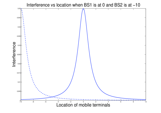
Figure 3: Interference as a function of location of mobile terminals when $\mathrm{BS}_{1}$ is at position $0$ (solid line) and $\mathrm{BS}_{2}$ at $-10$ (dotted line).

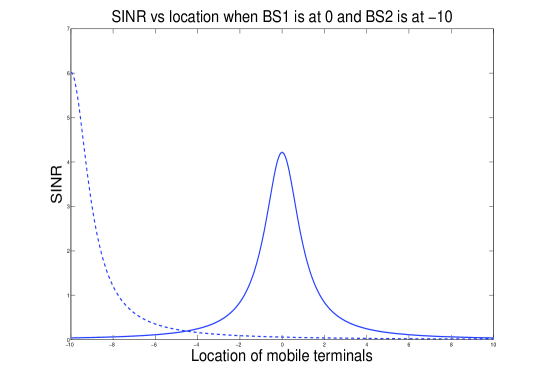
Figure 4: $\mathrm{SINR}$ as a function of location of mobile terminals when $\mathrm{BS}_{1}$ is at position $0$ (solid line) and $\mathrm{BS}_{2}$ at $-10$ (dotted line).

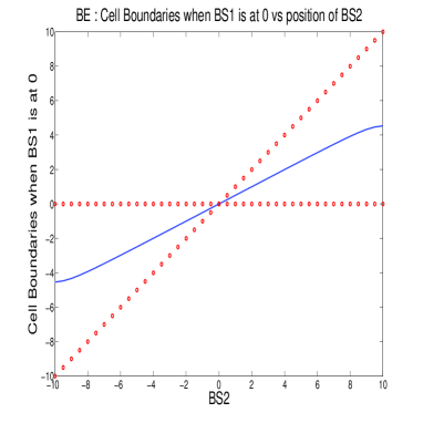
Figure 5: Wardrop Equilibrium: Thresholds determining the cell boundaries as a function of the location of the base stations. The network is deployed over the interval $[-10,10]$ (one-dimensional case) presented here vertically. We consider a uniform distribution of MTs and we find the threshold (solid line) determining the cell boundaries as a function of the base stations positions (dotted lines) by changing the position of one of them. $\mathrm{BS}_{1}$ is fixed at position $0$ and we change the position of $\mathrm{BS}_{2}$ from $-10$ to $+10$.

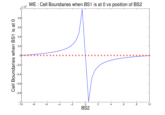
Figure 6: Worst Equilibrium: Thresholds determining the cell boundaries (vertical axis) that give the worst equilibrium in terms of the SINR as a function of the location of $\mathrm{BS}_{2}$ for $\mathrm{BS}_{1}$ at position $0$.

Notice that in problem $\mathrm{(P1)}$ if the functions $s_{i}\equiv 0$ the solution of the system $\mathrm{(S1)}$ becomes the well known Voronoi cells. In problem $\mathrm{(P2)}$ if we have that the functions $h_{i}\equiv 1$ we find again the Voronoi cells. In general however, the Voronoi configuration is far from being optimal.

4 Round Robin Scheduling Policy

We assume that a service provider wants to minimize the total power of the network while maintaining a certain average throughput of $\theta$ to each mobile terminal of the system using the round robin scheduling policy given by problem

$$(\mathrm{RR})\quad\operatorname*{Min}_{C_{i}}\sum_{i=1}^{K}\int\!\!\!\!\int_{C_{i}}\sigma^{2}(R^{2}+d_{i}(x,y)^{2})^{\xi/2}(2^{N_{i}\theta}-1)f(x,y)\,dx\,dy.$$ (34)

We see that this problem is an optimal transportation problem like the one in $\mathrm{(P1)}$ with cost function given by

$$F(d_{i}(x,y))=\sigma^{2}(R^{2}+d_{i}(x,y)^{2})^{\xi/2}\quad\text{and}$$ (35)

$$m_{i}(x,y)=(2^{N_{i}\theta}-1).$$ (36)

From the previous theorem, we can derive an explicit expression for this configuration.

Proposition.- There exist a unique optimum given by

$$C_{i}= \Big{\{}x_{0}\in\mathcal{D}\ :d_{i}(x_{0},y_{0})^{p}+h_{i}(N_{i})+N_{i}h_{i}^{\prime}(N_{i})$$

$$\leq d_{j}(x_{0},y_{0})^{p}+k_{j}(N_{j})+N_{j}k_{j}^{\prime}(N_{j}),\,\forall j\neq i\Big{\}}$$ (37)

$$N_{i}= \int\!\!\!\int_{C_{i}}f(x_{0},y_{0})\,dx_{0}\,dy_{0}.$$ (38)

Let’s see a direct application of our results:

Example 4.1

Consider a network of $N=2500$ mobile terminals distributed according to $f(x)$ in $[0,L]$ (for example, with $L=5.6$ miles for WiMAX radius cell). We consider two base stations at position $\mathrm{BS}_{1}=0$ and $\mathrm{BS}_{2}=L$ and $R=1$. Then, the mobile association threshold (the boundary between both cells, i.e., the location at which the mobile terminals obtain the same throughput by connecting to any of both base stations) is reduced to find $x$ such that the following equality holds:

$$(2^{N_{1}\theta}-1)(1+x^{2})f(x)+2^{N_{1}\theta}\theta\log 2\left[x+\frac{x^{3}}{3}\right]=$$

$$(2^{N_{2}\theta}-1)(1+(1-x)^{2})f(x)+2^{N_{2}\theta}\theta\log 2\left[\frac{4}{3}-2x+x^{2}-\frac{x^{3}}{3}\right]$$ (39)

Notice that this is a fixed point equation on $x$. If the mobile terminals are distributed uniformly, the optimal solution is given by $C_{1}=[0,1/2\leavevmode\nobreak\ L)$ and $C_{2}=[1/2\leavevmode\nobreak\ L,L]$, which is the solution that Voronoi cells would give us and in that case the number of mobile terminals connected to each base station would be given by

$$N_{1}=N_{2}=1250.$$ (40)

However, if the deployment distribution of the mobile terminals is more concentrated near $\mathrm{BS}_{2}$ than $\mathrm{BS}_{1}$, consider for example $f(x)=2x$, the optimal solution is given by $C_{1}=[0,q)$ and $C_{2}=[q,L]$ with $q=0.6027\leavevmode\nobreak\ L$ and

$$N_{1}=908\quad\textrm{and}\quad N_{2}=1592.$$ (41)

Notice that in the global optimization solution, the number of mobile terminals connected to $\mathrm{BS}_{1}$ is smaller that the number of mobile terminals connected to $\mathrm{BS}_{2}$. However, the cell size is bigger.

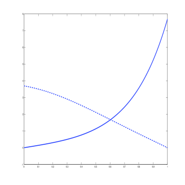
(a) Equilibrium in Non-Uniform distribution

Figure 7: Thresholds determining the cell boundaries (vertical axis) of the best equilibrium in terms of the SINR as a function of the location of $BS2$ for BS1 at position $0$ when we consider a non-homogeneous distribution given by $f(x)=(L-x)/2L^{2}$. Example: equilibrium when then distribution of mobile terminals is given by $f(x)=2x$ in the interval $[0,L]$ and the positions of the base stations are $\mathrm{BS}_{1}=0$ and $\mathrm{BS}_{2}=L$.

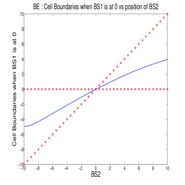
Figure 8: Wardrop Equilibrium in the Non-homogeneous case: The network is deployed over the interval $[-10,10]$ (one-dimensional case) presented here vertically. We find the threshold (solid line) determining the cell boundaries as a function of the base stations positions (dotted lines) by changing the position of one of them. $\mathrm{BS}_{1}$ is fixed at position $0$ and we change the position of $\mathrm{BS}_{2}$ from $-10$ to $+10$. The deployment distribution of the MTs is given by $f(x)=(L-x)/2L^{2}$.

5 Fairness problem

As we mention in section 2 the solution given by previous section 4 is optimal but may not be fair to all the mobile terminals since it will give higher throughput to the mobile terminals that are near the base stations. To deal with this problem we considered the fairness problem given by

$$\operatorname*{Min}\sum_{i=1}^{K}\int\!\!\!\!\int_{C_{i}}\frac{1}{\alpha-1}\left(\sigma^{2}(R^{2}+d^{2}_{i}(x,y))^{\xi/2}\right)^{\alpha-1}(2^{N_{i}\theta}-1)^{\alpha-1}f(x,y)\,dx\,dy.$$

As we can see this is also an optimal transportation problem $\mathrm{(P1)}$ where the functions considered in this setting are given by

$$F(d_{i}(x,y))=\frac{1}{\alpha-1}\left(\sigma^{2}(R^{2}+d^{2}_{i}(x,y))^{\xi/2}\right)^{\alpha-1}$$ (42)

$$m_{i}(x,y)=(2^{N_{i}\theta}-1)^{\alpha-1}.$$ (43)

Using Theorem 3.2 we are able to characterize the optimal cells for any $\alpha$ considered.

6 Rate fair allocation policy

In this framework, we give the possibility to mobile terminals to associate to the base station they prefer in order to minimize their power cost function while maintaining, as quality of service measurement, an average throughput of $\theta$.

As we presented in Section 2, this problem is equivalent to

$$(\mathrm{RF})\quad\operatorname*{Min}_{C_{i}}\sum_{i=1}^{K}\int\!\!\!\!\int_{C_{i}}\sigma^{2}(R^{2}+d^{2}_{i}(x,y))^{\xi/2}f(x,y)\,dx\,dy.$$ (44)

Notice that this problem is equivalent to $\mathrm{(P1)}$ where the functions

$$F(d_{i}(x,y))=\left(\sigma^{2}(R^{2}+d_{i}(x,y)^{2})^{\xi/2}\right),$$ (45)

and $s_{i}\equiv 1$. The problem has then a solution given by

Proposition.- There exist a unique optimum given by

$$\begin{array}[]{ll}C_{i}=&\Big{\{}x\in\mathcal{D}:\sigma^{2}(R^{2}+d^{2}_{i}(x_{0},y_{0}))^{\xi/2}\\ &\leq\sigma^{2}(R^{2}+d^{2}_{j}(x_{0},y_{0}))^{\xi/2},\forall j\neq i\Big{\}}\\ N_{i}=&\int\!\!\!\int_{C_{i}}f(x_{0},y_{0})\,dx_{0}\,dy_{0},\end{array}$$ (46)

which is represented by the Voronoi cells.

6.1 Penalization function

Notice that the penalization function or the case when the number of mobile terminals is greater than the number of carriers available in the cell in the rate fair allocation policy case is equivalent to $\mathrm{(P1)}$ where the functions

$$F(d_{i}(x,y))=\left(\sigma^{2}(R^{2}+d_{i}(x,y)^{2})^{\xi/2}\right).$$ (47)

$$s_{i}(N_{i})=\kappa_{i}(N_{i})=\left\{\begin{array}[]{cl}0&\textrm{ if }N_{i}\leq\mathrm{MAX}_{i},\\ \bar{\kappa}_{i}(N_{i}-\mathrm{MAX}_{i})&\textrm{ if }N_{i}>\mathrm{MAX}_{i}.\end{array}\right.$$ (48)

The problem has then a solution given by

Proposition.- There exist a unique optimum given by

$$\left\{\begin{array}[]{ll}C_{i}=&\big{\{}(x,y):\sigma^{2}(R^{2}+d^{2}_{i}(x_{0},y_{0}))^{\xi/2}+s_{i}(N_{i})+N_{i}\cdot s^{\prime}_{i}(N_{i})\\ &\leq\sigma^{2}(R^{2}+d^{2}_{i}(x_{0},y_{0}))^{\xi/2}+s_{j}(N_{j})+N_{j}\cdot s^{\prime}_{j}(N_{j})\big{\}}\\ N_{i}=&\int\!\!\!\int_{C_{i}}f(\omega,z)\,d\omega\,dz.\end{array}\right.$$ (49)

7 Performance Gap

As a second example consider again the case when the mobile terminals are uniformly distributed on $\mathcal{D}=[0,1]$ but this time the two antennas are located at coordinates $x_{1}=0$ and $x_{2}=1$. Consider the case when $p=1$ and

$$s_{1}(x)=100\quad\text{and}\quad s_{2}(x)=\left\{\begin{array}[]{ll}0&\quad\text{for}\quad 0\leq x\leq 0.999\\ 1&\quad\text{for}\quad 0.999\leq x\leq 1.\end{array}\right.$$

Then the equilibrium cell configuration $(C^{E}_{1},C^{E}_{2})$ is given by

$$C^{E}_{1}=\emptyset\quad\text{and}\quad C^{E}_{2}=[0,1],$$

and the optimum cell configuration $(C^{*}_{1},C^{*}_{2})$ is

$$C^{*}_{1}=[0,001[\quad\text{and}\quad C^{*}_{2}=]0.001,1].$$

The optimum is very unfair for mobile terminals living in the first cell $C^{*}_{1}$, who pay $x+100$, whereas the other mobile terminals just pay the distance from $1$. This is a toy example but it gives an idea of the performance gap between the centralized and the decentralized scenarios, also known as Price of Anarchy.

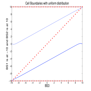
Figure 9: Wardrop Equilibrium with Multiple Base Stations: The grid area network is the interval $[-10,10]$ presented here vertically. We consider a uniform distribution of MTs. We find the threshold (solid and dashed lines) determining the cell boundaries as a function of the base stations positions (dotted lines) by changing the position of one of them. $\mathrm{BS}_{1}$ is fixed at position $-10$ and $\mathrm{BS}_{2}$ is fixed at position $10$ and we change the position of $\mathrm{BS}_{3}$ from $-10$ to $+10$.

8 Numerical Simulations

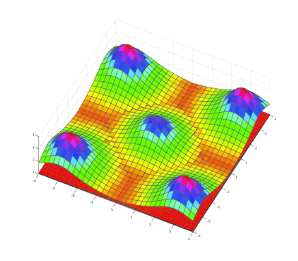
Figure 10: Wardrop Equilibrium in the 2D case: The grid area network is the square $[-4,4]\times[-4,4]$. We set the noise parameter $\sigma=0.3$ and we set four BSs at positions $\mathrm{BS}_{1}=(-3,-3)$ $\mathrm{BS}_{2}=(3,-3)$ $\mathrm{BS}_{3}=(3,3)$ $\mathrm{BS}_{4}=(-3,3)$ and one at the origin $\mathrm{BS}_{5}=(0,0)$. We determine the cell boundaries (deep lines) for the uniform distribution of users

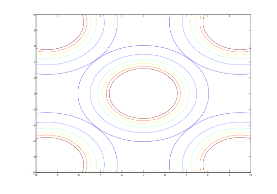
Figure 11: 2D case: Cell contours of the best equilibrium with uniform distribution of users.

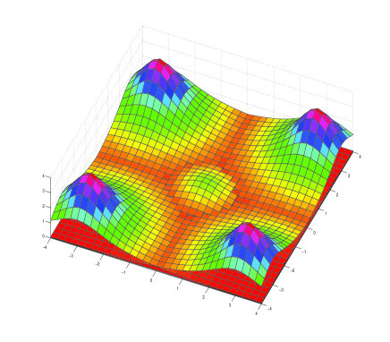
Figure 12: Wardrop Equilibrium in 2D Non-Uniform Case: The grid area network is the square $[-4,4]\times[-4,4]$. We set the noise parameter $\sigma=0.3$ and we set four BSs at positions $\mathrm{BS}_{1}=(-3,-3)$ $\mathrm{BS}_{2}=(3,-3)$ $\mathrm{BS}_{3}=(3,3)$ $\mathrm{BS}_{4}=(-3,3)$ and one at the origin $\mathrm{BS}_{5}=(0,0)$. We determine the cell boundaries (deep lines) for the non-uniform distribution of users given by $f(x,y)=(L^{2}-(x^{2}+y^{2}))/K$ where $K$ is a normalization factor. The latter situation takes into account when mobile terminals are more concentrated in the center and less concentrated in suburban areas.

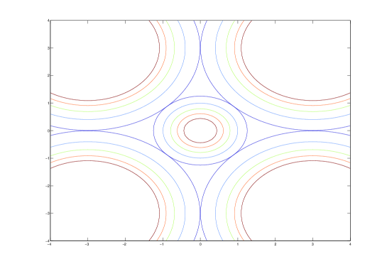
Figure 13: 2D Non-Uniform: Cell contours of the best equilibrium with non-uniform distribution of users.

In this section, we present several numerical results that validate our theoretical model.

8.1 One-dimensional case

We first consider the one-dimensional case and we consider a uniform distribution of users in the interval $[-10,10]$. We set the noise parameter $\sigma=0.3$. In Fig. 5, we fix one base station $\mathrm{BS}_{2}$ at position $0$ and take as parameter the position of base station $\mathrm{BS}_{1}$. We consider as path loss exponent $\xi=2$. Red lines shows the positions of the BSs. We are able to determine the cell boundary (solid blue curve) from $\mathrm{BS}_{1}$ and $\mathrm{BS}_{2}$ at different positions. In Fig. 9, we fix two base stations $\mathrm{BS}_{1}=-10$ and $\mathrm{BS}_{2}=10$ and we take as parameter the position of base station $\mathrm{BS}_{3}$. Red lines shows the positions of the BSs. We determine the cell boundary (solid blue curve) from $\mathrm{BS}_{1}$ and $\mathrm{BS}_{3}$ and the cell boundary (dotted blue curve) from $\mathrm{BS}_{2}$ and $\mathrm{BS}_{3}$.

8.2 Two-dimensional case: Uniform and Non-Uniform distribution of users

We consider the two-dimensional case. We consider the square $[-4,4]\times[-4,4]$ and the noise parameter $\sigma=0.3$. We set five base stations at positions $\mathrm{BS}_{1}=(-3,-3)$, $\mathrm{BS}_{2}=(3,-3)$, $\mathrm{BS}_{3}=(-3,3)$, $\mathrm{BS}_{4}=(3,3)$, and $\mathrm{BS}_{5}=(0,0)$. We determine the cell boundaries for the uniform distribution of MTs (see Fig. 11) and we compare it to the cell boundaries for the non-uniform distribution of MTs given by $f(x,y)=(L^{2}-(x^{2}+y^{2}))/K$ where $K$ is a normalization factor. The latter situation can be interpreted as the situation when mobile terminals are more concentrated in the center and less concentrated in suburban areas as in Paris, New York or London. We observe that the cell size of the base station $\mathrm{BS}_{5}$ at the center is smaller than the others at the suburban areas. This can be explained by the fact that as the density of users is more concentrated in the center the interference is greater in the center than in the suburban areas and then the $\mathrm{SINR}$ is smaller in the center. However the quantity of users is greater than in the suburban areas.

9 Conclusions and Future Perspectives

In the present work, we have studied the mobile association problem in the downlink scenario. The objective is to determine the spatial locations at which mobile terminals would prefer to connect to a given base station rather than to other base stations in the network if they were offered that possibility (denoted decentralized scenario). We are also interested in the spatial locations which are more convenient from a centralized or from a network operator point of view. In both approaches, the optimality depends upon the context. In the considered cases, we consider the minimization of the total power of the network, which can be considered as an energy-efficient objective, while maintaining a certain level of throughput for each user connected to the network. We have proposed a new approach using optimal transport theory for this mobile association problems and we have been able to characterize these mobile associations under different policies.

The present work can be extended in several different directions. One of these possible directions is to study the price of anarchy between the centralized and decentralized scenario. As we presented in Section 7, the considered example give us an indication that the price of anarchy should be unbounded but currently we don’t have precise bounds. The price of anarchy should be studied in both scenarios: the sum of a function and the multiplication. It should be interesting to study the application in the particular case when the network is an LTE network. Since our model is quite simplified in order to obtain exact solutions we could include the cases for the fading and shadowing effects. It is implicitly considered that the number of users in the network is stationary, but since at different times of the day there are different number of users, this management capabilities should be taken into account.

Appendix A

Consider the problem $\mathrm{(P1)}$

$$\operatorname*{Min}_{C_{i}}\sum_{i=1}^{K}\int\!\!\!\!\int_{C_{i}}\left[F(d_{i}(x,y))+s_{i}\left(\int\!\!\!\!\int_{C_{i}}f(\omega,z)\,d\omega\,dz\right)\right]f(x,y)\,dx\,\,dy,$$ (50)

where $C_{i}$ is the cell partition of $\mathcal{D}$. Suppose that $s_{i}$ are continuously differentiable, non-decreasing, and convex functions. The problem $\mathrm{(P1)}$ admits a solution that verifies

$$\mathrm{(S1)}\left\{\begin{array}[]{ll}C_{i}=&\big{\{}(x,y):F(d_{i}(x,y))+s_{i}(N_{i})+N_{i}\cdot s^{\prime}_{i}(N_{i})\\ &\leq F(d_{j}(x,y))+s_{j}(N_{j})+N_{j}\cdot s^{\prime}_{j}(N_{j})\big{\}}\\ N_{i}=&\int\!\!\!\int_{C_{i}}f(\omega,z)\,d\omega\,dz.\end{array}\right.$$ (51)

Proof.- The proof is based on Proposition 3.5 of Crippa et al. [15]. We include the proof for completeness and because part of it (mainly the existence of the solution) will be used in the proof of the following theorem. Notice that we have considered the case $F(d_{i}(x,y))=\lvert(x,y)-(x_{i},y_{i})\rvert^{p}$, but this holds for any continuous function $F$.

From Section 3, let us recall that Monge’s problem can be stated as follows: given two probability measures, $\mu$ and $\nu$, and a constant $p\geq 1$ we consider the minimization problem (denoted by $M_{p}(\mu,\nu)$):

$$M_{p}(\mu,\nu):=\inf\left\{\left(\int_{\mathcal{D}}\lvert x-T(x)\rvert^{p}\,d\mu(x)\right)^{1/p}\,:\,T:\mathcal{D}\to\mathcal{D}\,\,\textrm{Borel and such that}\,\,T\#\mu=\nu\right\}.$$ (52)

The relaxed formulation of Monge’s problem (denoted by $W_{p}(\mu,\nu)$) can be stated as follows

$$W_{p}(\mu,\nu):=\inf_{\gamma\in\Pi(\mu,\nu)}\left\{\left(\int_{\mathcal{D}\times\mathcal{D}}\lvert x-y\rvert^{p}\,d\gamma(x,y)\right)^{1/p}\right\},$$ (53)

where $\Pi(\mu,\nu)$ is the set of probability measures such that $\pi_{1}(\gamma)=\mu$ and $\pi_{2}(\gamma)=\nu$ where $\pi_{1}$ is the projection on the first component and $\pi_{2}$ is the projection on the second component.

If the probability measure $\mu$ can be written as $d\mu=f(x)\,dx$ (i.e. it is absolutely continuous with respect to the Lebesgue measure), then the optimal values of both problems coincide $M_{p}(\mu,\nu)=W_{F}(\mu,\nu)$, and there exists an optimal transport map from $\mu$ to $\nu$ which is unique $f$-a.e. if $p>1$. Another important characteristic of this relaxation is that it admits a dual formulation:

$$W_{p}^{p}(\mu,\nu)=\sup\left\{\int_{\mathcal{D}}u\,d\mu+\int_{\mathcal{D}}v\,d\nu:\begin{array}[]{c}u(x)+v(y)\leq\lvert x-y\rvert^{p}\quad\textrm{for}\,\mu\textrm{-a.e.}\,x\,\textrm{and}\,\nu\textrm{-a.e.}\,y\\ u\in L^{1}_{\mu}(\mathcal{D}),v\in L^{1}_{\nu}(\mathcal{D})\end{array}\right\}.$$ (54)

Moreover, there exists an optimal pair $(u,v)$ for this dual formulation, and when $\nu$ is an atomic probability measure (it can be written as $\nu=\sum_{i\in\mathbb{N}}b_{i}\delta_{y_{i}}$) the dual formulation becomes

$$W_{p}^{p}(\mu,\nu)=\sup\left\{\int_{\mathcal{D}}u\,d\mu+\sum_{i\in\mathbb{N}}b_{i}v(y_{i}):\begin{array}[]{c}u(x)+v(y_{i})\leq\lvert x-y_{i}\rvert^{p}\quad\textrm{for}\,\mu\textrm{-a.e.}\,x\,\textrm{and every}\,i\in\mathbb{N}\\ u\in L^{1}_{\mu}(\mathcal{D}),v\in L^{1}_{\nu}(\mathcal{D})\end{array}\right\}.$$ (55)

There exists another interesting characteristic when one of the measures is absolutely continuous with respect to the Lebesgue measure and the other measure is an atomic measure. If the probability measure $\mu$ can be written as $d\mu=f(x)\,dx$ where $f$ is a nonnegative function, $(y_{i})_{i\in\mathbb{N}}$ is a sequence of points in the domain $\mathcal{D}$ such that $\nu=\sum_{i\in\mathbb{N}}b_{i}\delta_{y_{i}}$, $(B_{i})_{i\in\mathbb{N}}$ is a partition of the domain such that the map $T(x)=\sum_{i\in\mathbb{N}}y_{i}\mathbf{1}_{B_{i}}(x)$ is an optimal transport map from $\mu$ to $\nu$, the pair $(u,v)$ is a solution of the dual formulation (54), then

$$u(x)=\inf_{i\in\mathbb{N}}(\lvert x-y_{i}\rvert^{p}-v(y_{i}))=\sum_{i\in\mathbb{N}}(\lvert x-y_{i}\rvert^{p}-v(y_{i}))\mathbf{1}_{B_{i}}(x)\,\textrm{for}\,f\textrm{-a.e.}\,x.$$ (56)

We also have a similar converse characteristic. If $(B_{i})_{i\in\mathbb{N}}$ is a partition of $\mathcal{D}$, we set $b_{i}=\int_{B_{i}}f(x)\,dx$, $\nu=\sum_{i\in\mathbb{N}}b_{i}\delta_{y_{i}}$ and $T(x)=\sum_{i\in\mathbb{N}}y_{i}\mathbf{1}_{B_{i}}(x)$, and there exists two functions $u\in L^{1}_{\mu}(\mathcal{D})$, $v\in L^{1}_{\nu}(\mathcal{D})$ satisfying the condition (56), then $T$ is optimal for $M_{p}(\mu,\nu)$ and the pair $(u,v)$ is optimal for the dual formulation (54).

In order to prove the existence and uniqueness of the solution we need to consider the following: We denote by $S$ the unit simplex in $\mathbb{R}^{k}$:

$$S=\left\{c=(c_{1},\ldots,c_{k})\in\mathbb{R}^{k}:\,c_{i}\geq 0,\,\sum_{i=1}^{k}c_{i}=1\right\}.$$ (57)

From Theorem 3.1, we deduce that

$$\inf_{\begin{subarray}{c}(A_{i})_{i\in\{1,\ldots,k\}}\\ \textrm{partition of}\,\mathcal{D}\end{subarray}}\left\{\sum_{i=1}^{k}\int_{A_{i}}\left[\lvert x-x_{i}\rvert^{p}+s_{i}\left(\int_{A_{i}}f(x)\,dx\right)\right]f(x)\,dx\right\}=\inf_{c\in S}\left\{W_{p}^{p}(f,\sum_{i=1}^{k}c_{i}\delta_{x_{i}})+\sum_{i=1}^{k}s_{i}(c_{i})c_{i}\right\}.$$ (58)

The function $F:S\to\mathbb{R}$ defined by $F(c_{1},\ldots,c_{k})=W_{p}^{p}\left(\mu,\sum_{i=1}^{k}c_{i}\delta_{x_{i}}\right)$ is continuous and convex.

If the functions $s_{i}$ are lower semi-continuous, then there exists an optimum and if in addition the maps $\eta_{i}(t):=th_{i}(t)$ are strictly convex, the optimum is unique.

We can then characterize the solution. If $(A_{i})_{i=1,\ldots,k}$ is an optimum, and $s_{i}$ are differentiable in $]0,1]$ and continuous in $0$, then the following holds:

$$C_{i}= \Big{\{}x\in\mathcal{D}\ :\lvert x-x_{i}\rvert^{p}+s_{i}(N_{i})+N_{i}s_{i}^{\prime}(N_{i})$$

$$\leq\lvert x-x_{j}\rvert^{p}+s_{j}(N_{j})+N_{j}s_{j}^{\prime}(N_{j}),\,\forall j\neq i\Big{\}}$$ (59)

$$N_{i}= \int_{C_{i}}f(x)\,dx.$$ (60)

Appendix B

Consider the problem $\mathrm{(P2)}$

$$\operatorname*{Min}_{C_{i}}\sum_{i=1}^{K}\int\!\!\!\!\int_{C_{i}}\left[F(d_{i}(x,y))\cdot m_{i}\left(\int\!\!\!\!\int_{C_{i}}f(\omega,z)\,d\omega\,dz\right)\right]\cdot f(x,y)\,dx\,dy,$$ (61)

where $C_{i}$ is the cell partition of $\mathcal{D}$. Suppose that $m_{i}$ are derivable. The problem $\mathrm{(P2)}$ admits a solution that verifies

$$\mathrm{(S2)}\left\{\begin{array}[]{ll}C_{i}=&\{x\,:\,m_{i}(N_{i})F(d_{i}(x,y))\,f(x,y)+U_{i}(x,y)\\ &\leq m_{j}(N_{j})F(d_{j}(x,y))\,f(x,y)+U_{j}(x,y)\}\\ U_{i}=&m^{\prime}_{i}(N_{i})\int\!\!\!\int_{C_{i}}F(d_{i}(x,y))f(x,y)\,dx\,dy\\ N_{i}=&\int\!\!\!\int_{C_{i}}f(\omega,z)\,d\omega\,dz.\end{array}\right.$$ (62)

Proof.- The proof is similar to Appendix A. The problem $\mathrm{(P2)}$ can be rewriten as follows:

$$\inf\left\{W_{c_{i}}\left(f\,dx,\sum_{i=1}^{k}c_{i}\delta_{x_{i}}\right):\,c_{i}\geq 0,\,\sum_{i=1}^{k}c_{i}=1\right\},$$ (63)

where

$$W_{c_{i}}\left(f\,dx,\sum_{i=1}^{k}c_{i}\delta_{x_{i}}\right)=\inf_{(A_{i})_{i=1}^{k}}\left\{\sum_{i=1}^{k}\int_{A_{i}}F(\lvert x-x_{i}\rvert)\cdot m_{i}(c_{i})f(x)\,dx:\int_{A_{i}}f\,dx=c_{i},(A_{i})_{i=1}^{k}\,\textrm{partition of}\,\mathcal{D}\right\}.$$ (64)

Let $\gamma$ be optimal for Monge-Kantorovich problem, then one can consider

$$\gamma(x,y)=\sum_{i=1}^{k}\gamma_{i}(x)\otimes\delta_{x_{i}}(y),\quad c_{i}=\gamma_{i}(\mathcal{D}),$$ (65)

where $\gamma_{i}$ is a positive measure such that $\gamma_{i}\leq f\,dx$

The function $F:S\to\mathbb{R}$ defined by $F(c_{1},\ldots,c_{k})=W_{p}^{p}\left(\mu,\sum_{i=1}^{k}c_{i}\delta_{x_{i}}\right)$ is lower semi-continuous. Then there exists a solution and it is unique almost surely.

Let $(c_{i})_{i=1}^{k}$ be a solution of $\mathrm{(P2)}$ and $(A_{i})_{i=1}^{k}$ the associated optimal partition. Let us fix two indices $i_{0}$, $j_{0}$ and a point $x_{0}\in A_{i_{0}}$. Let $\varepsilon\geq 0$. Let us consider the open ball of radius $\varepsilon$ and center $x_{0}$ that we denote as $B_{\epsilon}$. We denote its measure as $c_{\epsilon}$. We make a small variation of the optimal partition by taking from $A_{i_{0}}$ the ball $B_{\epsilon}$ and adding it to $A_{j_{0}}$. Since the partition $(A_{i})_{i=1}^{k}$ is optimal then

$$\int_{A_{i_{0}}}F(\lvert x-x_{i_{0}}\rvert)h_{i_{0}}(c_{i_{0}})f(x)\,dx+\int_{A_{j_{0}}}F(\lvert x-x_{j_{0}}\rvert)h_{j_{0}}(c_{j_{0}})f(x)\,dx$$

$$\leq\int_{A_{i_{0}}\setminus B_{\epsilon}}F(\lvert x-x_{i_{0}}\rvert)h_{i_{0}}(c_{i_{0}}-c_{\epsilon})f(x)\,dx+\int_{A_{j_{0}}\cup B_{\varepsilon}}F(\lvert x-x_{j_{0}}\rvert)h_{j_{0}}(c_{j_{0}}+c_{\varepsilon})f(x)\,dx,$$ (66)

which is equivalent to

$$\int_{A_{i_{0}}}F(\lvert x-x_{i_{0}}\rvert)(h_{i_{0}}(c_{i_{0}})-h_{i_{0}}(c_{i_{0}}-c_{\epsilon}))f(x)\,dx+\int_{B_{\epsilon}}F(\lvert x-x_{i_{0}}\rvert)h_{i_{0}}(c_{i_{0}}-c_{\epsilon})f(x)\,dx$$

$$\leq\int_{A_{j_{0}}}F(\lvert x-x_{i_{0}}\rvert)(h_{j_{0}}(c_{j_{0}}+c_{\epsilon})-h_{j_{0}}(c_{j_{0}}))f(x)\,dx+\int_{B_{\varepsilon}}F(\lvert x-x_{j_{0}}\rvert)h_{j_{0}}(c_{j_{0}}+c_{\varepsilon})f(x)\,dx.$$ (67)

Dividing the previous equation by $c_{\epsilon}$ and taking the limit when $\epsilon\to 0$, we obtain

$$\int_{A_{i_{0}}}F(\lvert x-x_{i_{0}}\rvert)h^{\prime}_{i_{0}}(c_{i_{0}})f(x)\,dx+F(\lvert x-x_{i_{0}}\rvert)h_{i_{0}}(c_{i_{0}})f(x_{0})$$

$$\leq\int_{A_{j_{0}}}F(\lvert x-x_{j_{0}}\rvert)h^{\prime}_{j_{0}}(c_{j_{0}})f(x)\,dx+F(\lvert x-x_{j_{0}}\rvert)h_{j_{0}}(c_{j_{0}})f(x_{0}).$$ (68)

Reorganizing the terms we obtain the desired result.

References

- [1] H. Hotelling, “Stability in competition,” The Economic Journal, vol. 39, no. 153, pp. 41–57, 1929.
- [2] F. Plastria, “Static competitive facility location: An overview of optimisation approaches,” European Journal of Operational Research, vol. 129, no. 3, pp. 461 – 470, 2001.
- [3] J. J. Gabszewicz and J.-F. Thisse, “Location,” in Handbook of Game Theory with Economic Applications (R. Aumann and S. Hart, eds.), vol. 1 of Handbook of Game Theory with Economic Applications, ch. 9, pp. 281–304, Elsevier, 1992.
- [4] E. Altman, A. Kumar, C. K. Singh, and R. Sundaresan, “Spatial SINR games combining base station placement and mobile association,” in INFOCOM, pp. 1629–1637, IEEE, 2009.
- [5] C. Villani, Optimal transport, vol. 338 of Grundlehren der Mathematischen Wissenschaften [Fundamental Principles of Mathematical Sciences]. Berlin: Springer-Verlag, 2009. Old and new.
- [6] G. Monge, “Mémoire sur la théorie des déblais et des remblais,” Histoire de l’Académie Royale des Sciences, 1871.
- [7] L. V. Kantorovich, “On the transfer of masses,” Dokl. Akad. Nauk., vol. 37, no. 2, pp. 227–229, 1942. Translated in Management Science, Vol. 5, pp. 1-4, 1959.
- [8] G. Buttazzo and F. Santambrogio, “A model for the optimal planning of an urban area,” SIAM J. Math. Anal., vol. 37, no. 2, pp. 514–530 (electronic), 2005.
- [9] G. Carlier and I. Ekeland, “The structure of cities,” J. Global Optim., vol. 29, no. 4, pp. 371–376, 2004.
- [10] G. Carlier and I. Ekeland, “Equilibrium structure of a bidimensional asymmetric city,” Nonlinear Anal. Real World Appl., vol. 8, no. 3, pp. 725–748, 2007.
- [11] Y. Yu, B. Danila, J. A. Marsh, and K. E. Bassler, “Optimal transport on wireless networks,” Mar. 28 2007. Comment: 5 pages, 4 figures.
- [12] F. Baccelli and B. Blaszczyszyn, Stochastic Geometry and Wireless Networks, Volume I - Theory, vol. 1 of Foundations and Trends in Networking Vol. 3: No 3-4, pp 249-449. NoW Publishers, 2009. Stochastic Geometry and Wireless Networks, Volume II - Applications; see http://hal.inria.fr/inria-00403040.
- [13] G. S. Kasbekar, E. Altman, and S. Sarkar, “A hierarchical spatial game over licenced resources,” in GameNets’09: Proceedings of the First ICST international conference on Game Theory for Networks, (Piscataway, NJ, USA), pp. 70–79, IEEE Press, 2009.
- [14] J. Wardrop, “Some theoretical aspects of road traffic research,” Proceedings of the Institution of Civil Engineers, Part II, vol. 1, no. 36, pp. 352–362, 1952.
- [15] G. Crippa, C. Jimenez, and A. Pratelli, “Optimum and equilibrium in a transport problem with queue penalization effect,” Adv. Calc. Var., vol. 2, no. 3, pp. 207–246, 2009.