Spatial-Dispersion Cancellation in Quantum Interferometry

Abstract

We investigate cancellation of spatial aberrations induced by an object placed in a quantum coincidence interferometer with type-II parametric down conversion as a light source. We analyze in detail the physical mechanism by which the cancellation occurs, and show that the aberration cancels only when the object resides in one particular plane within the apparatus. In addition, we show that for a special case of the apparatus it is possible to produce simultaneous cancellation of both even-order and odd-order aberrations in this plane.

I Introduction and background

I.1 Introduction

Aberration or spatial dispersion occurs when light passing through or reflecting off of an object gains unwanted phase-shifts that vary in the transverse spatial direction (orthogonal to the optical axis). These phase shifts are ”unwanted” in the sense that they differ from those obtained from Gaussian optics and cause distortions of the outgoing wavefronts. Mathematically, we can represent the aberrations by pure imaginary exponentials $e^{i\phi({\mathbf{x}})}$, where ${\mathbf{x}}$ is the transverse distance. Often $\phi({\mathbf{x}})$ may be expanded into a power series in $|{\mathbf{x}}|$ and separated into even and odd orders,

$$\phi({\mathbf{x}}) = \phi_{even}({\mathbf{x}})+\phi_{odd}({\mathbf{x}}),$$ (1)

$$\phi_{even}({\mathbf{x}}) = \sum_{j}a_{2j}r^{2j}P_{2j}(\theta),$$ (2)

$$\phi_{even}({\mathbf{x}}) = \sum_{j}a_{2j+1}r^{2j+1}P_{2j}(\theta).$$ (3)

Here, $r=|{\mathbf{x}}|$, while $P_{2j}(\theta)$ and $P_{2j+1}(\theta)$ are polynomials in $\sin\theta$ and/or $\cos\theta$. Usually, the expansion is expressed in terms of Seidel or Zernike polynomials (bornwolf (1, 2, 3)), but for our purposes the details of the expansion are not important. The important point here is simply that the even order terms are symmetric under reflection, $\phi_{even}({\mathbf{x}})=\phi_{even}(-{\mathbf{x}})$, while the odd terms are antisymmetric, $\phi_{odd}({\mathbf{x}})=-\phi_{odd}(-{\mathbf{x}})$.

In the papers bonato1 (4) and bonato2 (5), a particular type of interferometric device was described, and it was shown that if an object was placed in either arm of this device, then all even-order phase shifts introduced by the object will cancel in a temporal correlation experiment. The effect is very similar to the even-order frequency-dispersion cancellation first described in franson (6) and steinberg (7). As a light source, the aberration-cancellation experiment used photon pairs produced via spontaneous parametric downconversion (SPDC). The cancellation effect depended on the entanglement of the transverse spatial momenta in the resulting entangled photon pairs.

In this paper we reexamine the setup of bonato1 (4) and bonato2 (5) with two purposes in mind. After reviewing the apparatus and the even-order aberration cancellation effect in the next subsection, we first show (in section II) that for a special case of the apparatus we can in fact cancel all aberration, both even-order and odd-order. This cancellation only occurs when the sample is placed in one particular plane, and opens up the possibility of cancelling sample-induced abberation in dynamic light scattering berne (8, 9), fluorescence correlation spectroscopy maiti (10), or other temporal correlation-based experiments. Our second purpose (carried out in section III) is to analyze in more detail the results for the coincidence rate, in order to better understand the physical mechanisms involved in aberration cancellation. In section IV we discuss the conclusions that can be drawn from these results.

Note that, because we are motivated by the desire to cancel aberrations, we will use the phrase ”aberration-cancellation” for convenience throughout this paper, but in fact we mean the cancellation of all phase shifts arising in a given plane, not just the subset that differ from the predictions of Gaussian optics. In other words, ”aberration-cancellation” here means that only the intensity of the light is affected by the object, not the phase. So, for example, the placement in the object plane of an ideal lens, whose operation depends on second order phase shifts, should have no focusing power at this point; it will be as if the lens is not there.

I.2 Even-Order Aberration-Cancellation

Consider the setup shown in figure 1. In the main part of the apparatus, the two branches each consist of a Fourier transform system containing lenses of focal length $f$ and a sample providing a modulation $G_{j}({\mathbf{y}})$ of the beam, where $j=1,2$ labels the branch and ${\mathbf{y}}$ is the transverse distance from the optic axis. The $G_{j}$ represent objects or samples whose properties we wish to analyze, and the goal is to cancel optical aberrations introduced by the samples. The case where there is a sample only in branch 1 is included by simply setting $G_{2}=1$, but we will keep the more general two-sample case; we will see later that the extra generality pays off by allowing useful additional effects. A controllable time delay $\tau$ is inserted in one arm of the interferometer. Since we will be referring to it often, we give a name to the plane containing the samples, denoting this plane by $\Pi$. The $\Pi$-plane is simultaneously the back focal plane of the first lens and the front focal plane of the second. The two lenses together form a 4f Fourier transform system. We will examine in a later section what happens when the sample is moved out of the $\Pi$-plane. Throughout this paper, we assume that the sample is of negligible thickness compared to all of the other distances involved in the apparatus. We will refer to the photon in the upper branch (branch 1) as the signal and the photon in branch 2 as the idler. The polarizing beam splitter sends the horizontally polarized photon into the upper (signal) branch and the vertically polarized photon into the lower (idler) branch.

Photons are fed into the system by a continuous wave laser which pumps a $\chi^{(2)}$ nonlinear crystal, leading to collinear type II parametric downconversion. The frequencies of the two photons are $\Omega_{0}\pm\nu$, while the transverse momenta are $\pm{\mathbf{q}}$. For simplicity, assume the frequency bandwidth is narrow compared to $\Omega_{0}$. The two photons have total wavenumbers ${{\Omega_{0}\pm\nu}\over c}$, which will be approximated by $k={{\Omega_{0}}\over c}$ where appropriate. The downconversion spectrum is given by

$$\Phi({\mathbf{q}},\nu)=sinc\left[{{L\Delta({\mathbf{q}},\nu)}\over 2}\right]e^{i{{L\Delta({\mathbf{q}},\nu)}\over 2}}.$$ (4)

Here, $L$ is the thickness of the nonlinear crystal and for type-II downconversion we have

$$\Delta({\mathbf{q}},\nu)=-\nu D+M\hat{\mathbf{e}_{2}}\cdot{\mathbf{q}}+{{2|{\mathbf{q}}|^{2}}\over{k_{pump}}}.$$ (5)

$D$ is the difference between the group velocities of the ordinary and extraordinary waves in the crystal, and $M$ is the spatial walk-off in the direction $\hat{{\mathbf{e}_{2}}}$ perpendicular to the interferometer plane. The last term in $\Delta$ is due to diffraction as the wave propagates through the crystal.

The parametric downconversion process may be described by a Hamiltonian of the form

$$\hat{H}=i\hbar\chi\hat{a}_{s}^{\dagger}\hat{a}_{i}^{\dagger}+H.C.,$$ (6)

where $\hat{a}_{s}$ and $\hat{a}_{i}$ are annihilation operators for the signal and idler photons. The constant $\chi$ includes the amplitude of the classical pump field. Applying the time evolution operator $e^{-i\hat{H}t/\hbar}$ to the vacuum state, we find that the wavefunction entering the apparatus from the crystal can be written as

$$|\Psi(t)\rangle=(1-|\eta|^{2}/2)|0\rangle+\eta|\Psi_{2}\rangle+\eta^{2}|\Psi_{4}\rangle+\dots,$$ (7)

where $\eta=\chi t$, and $|\Psi_{2n}\rangle$ represents a term with $n$ photons in the signal mode and $n$ in the idler mode. For parametric downconversion we operate in the regime where $|\eta|<<1$, so that terms higher than $|\Psi_{2}\rangle$ may be neglected. In addition, the vacuum term may be ignored since it will not contribute to coincidence detection. Thus, effectively our wavefunction is given by

$$|\Psi\rangle\approx|\Psi_{2}\rangle=\int dq\;d\nu\;\Phi({\mathbf{q}},\nu)\hat{a}_{s}^{\dagger}({\mathbf{q}},\Omega_{0}+\nu)\hat{a}_{i}^{\dagger}(-{\mathbf{q}},\Omega_{0}-\nu)|0\rangle.$$ (8)

Note that $G_{1}$ and $G_{2}$ could be produced by two separate objects at two separate points in space, in which case we would need to use a polarizing beam splitter (PBS) to separate the incoming beams. Alternatively, $G_{1}$ and $G_{2}$ could both be produced by a single object which acts differently on the two polarization states, in which case we could dispense with the PBS.

In the detection stage, two bucket detectors $D_{1}$ and $D_{2}$ are connected in coincidence. We add adjustable irises with aperture functions $p_{1}({\mathbf{x}}_{1})$ and $p_{2}({\mathbf{x}}_{2})$ in front of the detectors. We will end up taking these apertures to be of infinite width, but initially we leave them in, for reasons to be explained below. A lens of focal length $f_{d}$ is placed one focal length in front of each detector. The distances from the Fourier plane of the main part of the apparatus to the aperture and from the aperture to the lens are $d_{1}$ and $d_{2}$. In order to erase path information for the photons reaching each detector, a polarizer at $45^{\circ}$ to the polarization directions of both incoming beams is placed in each path. The two polarizers are oriented orthogonal to each other.

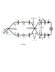
Figure 1: (Color online) Schematic view of aberration-cancellation setup. (Distances and angles not necessarily drawn in correct proportions.) The horizontally polarized signal travels in the upper branch and experiences modulation $G_{1}$, while the vertically polarized idler experiences modulation $G_{2}$ in the lower branch. $G_{1}$ and $G_{2}$ are both located in the plane $\Pi$, halfway between the lenses of focal length $f$. The beam splitter mixes the beams before they reach the detectors $D_{1}$ and $D_{2}$, which are connected by a coincidence circuit.

The full transfer function for each branch is bonato2 (5)

$$H_{j\alpha}({\mathbf{x}_{\alpha}},{\mathbf{q}_{j}},\omega)=G_{j}({f\over k}{\mathbf{q}_{j}})H_{D_{\alpha}}({\mathbf{x}_{\alpha}},{\mathbf{q}_{j}},\omega),$$ (9)

where the transfer function of the detection stage is

$$H_{D_{\alpha}}({\mathbf{x}_{\alpha}},{\mathbf{q}_{j}},\omega) = e^{ik(d_{1}+d_{2}+f_{D})}e^{-{{ik}\over{2f_{D}}}\left({{d_{2}}\over{f_{D}}}-1\right){\mathbf{x}_{\alpha}}^{2}}$$ (10)

$$\quad\cdot e^{-{{id_{1}}\over{2k}}{\mathbf{q}_{j}}^{2}}\tilde{\cal P}_{\alpha}\left({k\over{f_{D}}}{\mathbf{x}_{\alpha}}-{\mathbf{q}_{j}}\right).$$

$\tilde{\cal P}_{\alpha}$ is the Fourier transform of the aperture function,

$$\tilde{\cal P}_{\alpha}\left({k\over{f_{D}}}{\mathbf{x}_{\alpha}}-{\mathbf{q}_{j}}\right)=\int d^{2}x^{\prime}p_{\alpha}({\mathbf{x}}^{\prime})e^{-i\left({k\over{f_{D}}}{\mathbf{x}_{\alpha}}-{\mathbf{q}_{j}}\right)\cdot{\mathbf{x}^{\prime}}},$$ (11)

with $\alpha=\{1,2\}$ labelling the detector and $j=\{s,i\}$ labelling the signal or idler branch. In these expressions, $k$ is the longitudinal wavenumber, $k=\sqrt{(\omega/c)^{2}-q^{2}}\approx{\omega\over c}$ for $|{\mathbf{q}}|<<k$.

The nonpolarizing beam splitter mixes the incident beams, so each detector sees a superposition of the signal and idler beams. The positive-frequency part of the field entering detector $\alpha$ is given by

$$E_{\alpha}^{(+)}({\mathbf{x}}_{\alpha},t_{\alpha}) = \int dqd\omega e^{-i\omega t_{\alpha}}\left[H_{s\alpha}({\mathbf{x}_{\alpha}},{\mathbf{q}_{s}},\omega)\hat{a}_{s}({\mathbf{q}}_{s},\omega)\right.$$ (12)

$$\left.\quad+H_{i\alpha}({\mathbf{x}_{\alpha}},{\mathbf{q}_{i}},\omega)\hat{a}_{i}({\mathbf{q}}_{i},\omega)\right].$$

Using this field, we can compute the amplitude for coincidence detection:

$$A({\mathbf{x}}_{1},{\mathbf{x}}_{2},t_{1},t_{2})=\langle 0|E_{1}^{(+)}({\mathbf{x}}_{1},t_{1})E_{2}^{(+)}({\mathbf{x}}_{2},t_{2})|\Psi\rangle$$

$$\;=\int d^{2}q\;d\nu\;\Phi({\mathbf{q}},\nu)$$ (13)

$$\;\times\left[e^{-i(\Omega_{o}+\nu)t_{1}}e^{-i(\Omega_{o}-\nu)t_{2}}H_{s1}({\mathbf{x}}_{1},{\mathbf{q}},\nu)H_{i2}({\mathbf{x}}_{2},-{\mathbf{q}},-\nu)\right.$$

$$\;+\left.e^{-i(\Omega_{o}-\nu)t_{1}}e^{-i(\Omega_{o}+\nu)t_{2}}H_{i1}({\mathbf{x}}_{1},-{\mathbf{q}},-\nu)H_{s2}({\mathbf{x}}_{2},{\mathbf{q}},\nu)\right],$$

where $H_{j\alpha}({\mathbf{x}}_{\alpha},{\mathbf{q}}_{j},\Omega_{0}\pm\nu)$ have been abbreviated by $H_{j\alpha}({\mathbf{x}}_{\alpha},{\mathbf{q}}_{j},\pm\nu)$.

The coincidence rate as a function of time delay $\tau$ is

$$R(\tau)\;=\;\int d^{2}x_{1}d^{2}x_{2}dt_{1}dt_{2}|A({\mathbf{x}}_{1},{\mathbf{x}}_{2},t_{1},t_{2})|^{2}.$$ (14)

As was shown in rubin (11), $R(\tau)$ will generically be of the form

$$R(\tau)=R_{0}\left[1-\Lambda\left(1-{{2\tau}\over{DL}}\right)W(\tau)\right].$$ (15)

where $\Lambda(x)$ is the triangular function:

$$\Lambda(x)=\bigg{\{}\begin{array}[]{l}1-|x|,\qquad|x|\leq 1\\ 0,\qquad\qquad|x|>1\end{array}$$ (16)

The $\tau$-independent background term $R_{0}$ and $\tau$-dependent modulation term $W(\tau)$ were calculated in bonato2 (5) to be:

$$R_{0} = \int d^{2}qd^{2}q^{\prime}sinc[ML{\mathbf{e}}_{2}\cdot({\mathbf{q}}-{\mathbf{q}^{\prime}})]$$ (17)

$$\times\;G_{1}^{\ast}\left({{f{\mathbf{q}}}\over k}\right)G_{2}^{\ast}\left(-{{f{\mathbf{q}}}\over k}\right)G_{1}\left({{f{\mathbf{q}^{\prime}}}\over k}\right)G_{2}\left(-{{f{\mathbf{q}^{\prime}}}\over k}\right)$$

$$\times\;\tilde{\cal P}_{1}({\mathbf{q}}-{\mathbf{q}^{\prime}})\tilde{\cal P}_{2}(-{\mathbf{q}}+{\mathbf{q}^{\prime}})$$

$$\times\;e^{-{{iML}\over 2}{\mathbf{e}_{2}}\cdot({\mathbf{q}}-{\mathbf{q}^{\prime}})}e^{{{2id_{1}\over{k_{pump}}}}({\mathbf{q}}^{2}-{\mathbf{q}^{\prime 2}})}$$

$$W(\tau) = {1\over{R_{0}}}\int d^{2}qd^{2}q^{\prime}sinc\left[MLe_{2}\cdot({\mathbf{q}}+{\mathbf{q}^{\prime}})\Lambda\left(1-{{2\tau}\over{DL}}\right)\right]$$ (18)

$$\times\;G_{1}^{\ast}\left({{f{\mathbf{q}}}\over k}\right)G_{2}^{\ast}\left(-{{f{\mathbf{q}}}\over k}\right)G_{1}\left({{f{\mathbf{q}^{\prime}}}\over k}\right)G_{2}\left(-{{f{\mathbf{q}^{\prime}}}\over k}\right)$$

$$\times\;\tilde{\cal P}_{1}({\mathbf{q}}+{\mathbf{q}^{\prime}})\tilde{\cal P}_{2}(-{\mathbf{q}}-{\mathbf{q}^{\prime}})$$

$$\times\;e^{-{{iM}\over D}\tau{\mathbf{e}_{2}}\cdot({\mathbf{\mathbf{q}}}-{\mathbf{\mathbf{q}^{\prime}}})}e^{{{2id_{1}\over{k_{pump}}}}({\mathbf{q}}^{2}-{\mathbf{q}^{\prime 2}})}.$$

Now let the apertures be large, so that the $\tilde{\cal P}_{j}$ become delta functions, reducing equations (17) and 18 to:

$$R_{0} = \int d^{2}q\left|G_{1}\left({{f{\mathbf{q}}}\over k}\right)G_{2}\left(-{{f{\mathbf{q}}}\over k}\right)\right|^{2}$$ (19)

$$W(\tau) = {1\over{R_{0}}}\int d^{2}qe^{-{{2iM\tau}\over D}{\mathbf{e}_{2}}\cdot{\mathbf{q}}}G_{1}^{\ast}\left({{f{\mathbf{q}}}\over k}\right)G_{1}\left(-{{f{\mathbf{q}}}\over k}\right)$$ (20)

$$\qquad\times\;G_{2}^{\ast}\left(-{{f{\mathbf{q}}}\over k}\right)G_{2}\left({{f{\mathbf{q}}}\over k}\right).$$

Suppose that $G_{j}({\mathbf{x}})=t_{j}({\mathbf{x}})e^{i\phi_{j}({\mathbf{x}})}$, where $t_{j}$ is real and the effects of aberrations are contained in the phase factor $\phi_{j}$. Disregarding the background term for the moment, we see from the presence in equation (20) of the factors

$$G_{1}^{\ast}\left({{f{\mathbf{q}}}\over k}\right)G_{1}\left(-{{f{\mathbf{q}}}\over k}\right)$$

$$\quad=t_{1}^{\ast}\left({{f{\mathbf{q}}}\over k}\right)t_{1}\left(-{{f{\mathbf{q}}}\over k}\right)e^{-i\left[\phi_{1}\left({{f{\mathbf{q}}}\over k}\right)-\phi_{1}\left(-{{f{\mathbf{q}}}\over k}\right)\right]}$$ (21)

that even order aberration terms arising from sample 1 cancel from the modulation term. The even order aberrations from sample 2 cancel similarly. This is the even order cancellation effect of references bonato1 (4) and bonato2 (5).

It should be remarked that the setup of figure 1 may be simplified by removing the lenses immediately in front of the detectors. We have left both the lenses and the apertures in the setup because together they lead to the presence of the Fourier transformed aperture functions $\tilde{\cal P}_{j}$ in equations (17) and (18); the delta functions that arise from the $\tilde{\cal P}_{j}$ when the apertures become large will serve as convenient bookkeeping devices in the following sections as we trace various terms back to their origins. If we choose to simplify the apparatus and remove the lenses, then equation (10) will be replaced by

$$H_{D_{\alpha}}({\mathbf{x}}_{\alpha},{\mathbf{q}}_{j},\omega) = e^{ik(d_{1}+d)}e^{{-id_{1}{\mathbf{q}}^{2}_{j}}\over{2k}}$$

$$\;\times\;\int p({\mathbf{x}^{\prime}})e^{{{ik}\over{2d}}({\mathbf{x}^{\prime}}-{\mathbf{x}}_{\alpha})^{2}}e^{i{\mathbf{q}}\cdot{\mathbf{x}^{\prime}}}d^{2}x^{\prime},$$

where $d$ is the total aperture-to-detector distance, with corresponding changes in equations (17) and (18). However, in the large-aperture limit this does not affect the coincidence rate, which will still be given by expressions (15), (19), and (20).

II All-order cancellation

II.1 Aberration cancellation to all orders

Now, consider the background term $R_{0}$ in equation (19). It depends on $G_{1}$ and $G_{2}$ only through the squared modulus of each. Thus any phase changes introduced by $G_{1}$ or $G_{2}$ cancel completely; in particular, the background term $R_{0}$ exhibits cancellation of aberrations of all orders, not just even orders. In the current situation, this $R_{0}$ is of no importance, simply being a constant and having no effect on the $\tau$-dependence of the correlation. However, the fact that all orders of aberration can be cancelled in the background term raises the question as to whether it can be arranged for this to happen in the modulation term as well.

It turns out that the answer to this question is positive: it is possible to use this apparatus to cancel all aberrations induced by a thin sample, of both even and odd orders. The means for doing so is evident from examining equation (20). Suppose that $G_{1}({\mathbf{x}})=G_{2}({\mathbf{x}})$, as shown schematically in figure 2. This can can happen in one of two ways: either two identical samples may be placed in the two arms, or it may be arranged so that the two beams both pass through the same sample; in either case it is necessary for the sample to act in the same manner on both polarization states. The second possibility will usually be of more practical interest, since identical samples will often not be available. For $G_{1}=G_{2}$, equations (17) and (18) give

$$R_{0} = \int d^{2}q\left|G_{1}\left({{f{\mathbf{q}}}\over k}\right)G_{1}\left(-{{f{\mathbf{q}}}\over k}\right)\right|^{2}$$ (23)

$$W(\tau) = {1\over{R_{0}}}\int d^{2}qe^{-{{2iM\tau\hat{\mathbf{e}_{2}}\cdot{\mathbf{q}}}\over D}}\left|G_{1}\left({{f{\mathbf{q}}}\over k}\right)G_{1}\left(-{{f{\mathbf{q}}}\over k}\right)\right|^{2}$$ (24)

Setting $G_{1}({\mathbf{x}})=t({\mathbf{x}})e^{i\phi({\mathbf{x}})},$ we see that all phases now cancel from the $\tau$-modulated term $W$. Thus, all aberrations induced by the sample, of any order, will completely cancel from the coincidence rate.

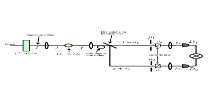
Figure 2: (Color online) Schematic view of apparatus in figure 1, with $G_{1}$ set equal to $G_{2}$. (Distances and angles not necessarily drawn in correct proportions.) Here $G_{1}$ and $G_{2}$ are being produced by a single object. The signal and idler are collinear. It is also possible for $G_{2}$ and $G_{2}$ to be produced by two identical but spatially separate objects interacting with noncollinear signal and idler.

II.2 Condition for All-Order Cancellation

Up to this point, we have assumed that the objects providing the modulation were located in the plane labelled $\Pi$ in figure 1. Now we consider what happens if the modulation objects (the samples) are moved out of the $\Pi$-plane by some distance $z\neq 0$. Consider a single arm of the apparatus, as shown in figure 3. We will take the distance $z$ from $\Pi$ to be positive if the sample is moved toward the source, and negative if moved toward the detector. Now, the impulse response functions for the first and second lens respectively in each branch of the system will be:

$$h_{1}({\mathbf{\xi}},{\mathbf{y}}) = {1\over{i\lambda f}}\cdot{1\over{i\lambda(f-z)}}\int e^{{{ik}\over 2}\left({{{\mathbf{y}}^{2}}\over{f-z}}+{{{\mathbf{\xi}}^{2}}\over f}\right)}$$ (25)

$$\times\;e^{{{ik}\over 2}\left({1\over{f-z}}\right){\mathbf{x}^{\prime 2}}}e^{-ik{\mathbf{x}^{\prime}}\cdot\left({{\mathbf{y}}\over{f-z}}+{{\mathbf{\xi}}\over f}\right)}\;d^{2}x^{\prime}$$

$$h_{2}({\mathbf{y}},{\mathbf{x}}) = {1\over{i\lambda f}}\cdot{1\over{i\lambda(f+z)}}\int e^{{{ik}\over 2}\left({{{\mathbf{y}}^{2}}\over{f+z}}+{{{\mathbf{x}}^{2}}\over f}\right)}$$ (26)

$$\times\;e^{{{ik}\over 2}\left({1\over{f+z}}\right){\mathbf{x}}^{\prime\prime 2}}e^{-ik{\mathbf{x}^{\prime\prime}}\cdot\left({{\mathbf{y}}\over{f+z}}+{{\mathbf{x}}\over f}\right)}\;d^{2}x^{\prime\prime}$$

${\mathbf{y}}$, ${\mathbf{x}^{\prime}}$, ${\mathbf{x}^{\prime\prime}}$, and ${\mathbf{\xi}}$ are the transverse distances at the points shown in figure 2. The integrals can be carried out, giving us the result that:

$$h_{1}({\mathbf{\xi}},{\mathbf{y}}) = {1\over{i\lambda f}}e^{{{ik}\over{2f}}\left[{z\over f}{\mathbf{\xi}}^{2}-2{\mathbf{\xi}}\cdot{\mathbf{y}}\right]}$$ (27)

$$h_{2}({\mathbf{y}},{\mathbf{x}}) = {1\over{i\lambda f}}e^{-{{ik}\over{2f}}\left[{z\over f}{\mathbf{x}}^{2}+2{\mathbf{x}}\cdot{\mathbf{y}}\right]}\;=\;-h_{1}^{\ast}(-{\mathbf{x}},{\mathbf{y}}).$$ (28)

So the impulse response for one branch of the apparatus from source to Fourier plane (not including the detection stage) is

$$h_{j}^{\prime}({\mathbf{\xi}},{\mathbf{x}}) = \int h_{1}({\mathbf{\xi}},{\mathbf{y}})G_{j}({\mathbf{y}})h_{2}({\mathbf{y}},{\mathbf{x}})d^{2}y$$ (29)

$$= {{e^{{{ik}\over{2f^{2}}}z({\mathbf{\xi}}^{2}-{\mathbf{x}}^{2})}}\over{(i\lambda f)^{2}}}\int e^{-{{ik}\over{f}}\left({\mathbf{\xi}}+{\mathbf{x}}\right)\cdot{\mathbf{y}}}G_{j}({\mathbf{y}})d^{2}y.$$ (30)

Fourier transforming to find the transfer function leads to:

$$H_{j}^{\prime}({\mathbf{x}},{\mathbf{q}},\omega) = \int h({\mathbf{\xi}},{\mathbf{x}})\;e^{i{\mathbf{q}}\cdot{\mathbf{\xi}}}d^{2}\xi$$ (33)

$$= {1\over{(i\lambda f)^{2}}}\int d^{2}y\;G_{j}({\mathbf{y}})\;e^{-{{ik}\over f}{\mathbf{x}}\cdot{\mathbf{y}}}e^{-{{ik}\over{2f^{2}}}z{\mathbf{x}}^{2}}$$

$$\qquad\times\int d^{2}{\mathbf{\xi}}\;e^{{{ikz}\over{2f^{2}}}{\mathbf{\xi}}^{2}}e^{i{\mathbf{\xi}}\left({\mathbf{q}}-{{k{\mathbf{x}}}\over f}\right)}$$

$$= -{1\over{\lambda z}}e^{-i{\mathbf{q}}\cdot{\mathbf{x}}}\int d^{2}y\;G_{j}\left({\mathbf{y}}+{{f{\mathbf{q}}}\over k}\right)$$

$$\qquad\times\;e^{-{{ik}\over f}{\mathbf{x}}\cdot{\mathbf{y}}}e^{-{{ik}\over{2z}}{\mathbf{y}}^{2}}e^{-{{ikz}\over{2f^{2}}}{\mathbf{x}}^{2}}.$$

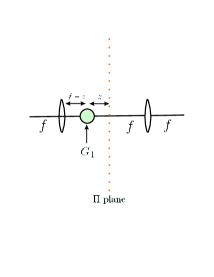
Figure 3: (Color online) Blown up version of a portion of one branch from apparatus of figure 1 (or figure 2), with the object moved a distance $z$ out of the central plane, $\Pi$.

Previously, for $z=0$, this transfer function was simply given by

$$H_{j}^{\prime}({\mathbf{x}},{\mathbf{q}},\omega)=(constants)\cdot G_{j}\left({{f{\mathbf{q}}}\over k}\right)e^{-i{\mathbf{q}}\cdot{\mathbf{x}}}.$$ (34)

Therefore, for $z\neq 0$, we must make the replacement (up to overall constants)

$$G\left({{f{\mathbf{q}}}\over k}\right) \longrightarrow \int d^{2}y\;G\left({\mathbf{y}}+{{f{\mathbf{q}}}\over k}\right)$$

$$\qquad\times\;e^{-{{ik}\over f}{\mathbf{x}}\cdot{\mathbf{y}}}e^{-{{ikz}\over{2f^{2}}}{\mathbf{x}}^{2}}\left({1\over z}e^{-{{ik}\over{2z}}{\mathbf{y}}^{2}}\right)$$

in all previous results, and equation (9) now involves an integral instead of a simple product. (For $z=0$, the factors in the last set of parentheses become proportional to $\delta^{(2)}({\mathbf{y}})$, leading back to the previous results.) In particular, in equations (23) and (24), the factor $\left|G_{1}\left({{f{\mathbf{q}}}\over k}\right)\right|^{2}$ becomes

$$\int d^{2}y\;d^{2}y^{\prime}\;G_{1}\left({\mathbf{y}}+{f\over{f_{D}}}{\mathbf{x}}\right)G_{1}^{\ast}\left({\mathbf{y}}^{\prime}+{f\over{f_{D}}}{\mathbf{x}}\right)e^{-{{ik}\over{2z}}({\mathbf{y}}^{2}-{\mathbf{y}^{\prime 2}})}.$$ (36)

Clearly, the phase of $G_{1}$ no longer cancels out of this expression since nothing forces ${\mathbf{y}}$ to equal ${\mathbf{y}^{\prime}}$. The arguments of the two factors of $G_{1}$ are now unrelated, so that aberration cancellation no longer occurs.

So any cancellation that occurs can hold exactly only for phases arising in the $\Pi$-plane of the Fourier transform system. The cancellation is approximate in the vicinity of this plane. For samples of finite thickness, the degree of approximate cancellation will diminish as the thickness increases.

Defining ${\mathbf{\epsilon}}={\mathbf{y}}-{\mathbf{y}^{\prime}}$, the exponential term in equation (36) becomes

$$e^{-{{ik}\over{2z}}\left(2{\mathbf{\epsilon}}\cdot{\mathbf{y}}-{\mathbf{\epsilon}}^{2}\right)}.$$ (37)

Assuming that $G_{1}^{\ast}\left({\mathbf{y}}-\epsilon+{f\over{f_{d}}}{\mathbf{x}}\right)$ is slowly varying in ${\mathbf{\epsilon}}$ compared to the variation of the exponential, we may obtain an estimate of the distance $z$ over which the sample may be moved out of the plane while still maintaining a high degree of abberation cancellation. The aberration cancels when ${\mathbf{\epsilon}}=0$, so we may use the maximum size of ${\mathbf{\epsilon}}$ as a measure of the degree of failure of the aberration cancellation. As $z\to 0$, the rapid oscillations of the exponential term cause the integral of equation (36) to go to zero, unless $k\left|2{\mathbf{\epsilon}}\cdot{\mathbf{y}}-{\mathbf{\epsilon}}^{2}\right|$ also goes to zero at least as fast as $|z|$. So, we must have

$$\left|2{\mathbf{\epsilon}}\cdot{\mathbf{y}}-{\mathbf{\epsilon}}^{2}\right|\lesssim\left|{z\over k}\right|\sim|z\lambda|.$$ (38)

From this, we have

$$|z|\sim{{{\mathbf{\epsilon}}_{M}\;|{\mathbf{y}}|}\over\lambda},$$ (39)

where ${\mathbf{\epsilon}}_{M}$ is the maximum value of ${\mathbf{\epsilon}}$. Let $r_{s}$ be the maximum illuminated radius of the sample. Then, by requiring that $|{\mathbf{\epsilon}}_{M}|<<r_{s}$, we have the estimate that

$$|z|<<{{r_{s}^{2}}\over\lambda}.$$ (40)

This is essentially a limit on how far from stationarity we may be and still safely apply a stationary-phase approximation. Actually, we may make this limit a bit more precise. Since two sample points ${\mathbf{y}}$ and ${\mathbf{y}^{\prime}}$ inside the Airy disk of the lens can not be distinguished from each other, we may require that $|{\mathbf{\epsilon}}_{M}|\sim R_{airy}$, where

$$R_{airy}={{1.22f\lambda}\over a}$$ (41)

is the radius of the Airy disk. By substituting this into equation (39), we can thus conclude that, at most, the order of magnitude of $|z|$ may be given by

$$|z|\lesssim{{fr_{s}}\over a}.$$ (42)

Taking for example the values $r_{s}\sim 10^{-4}m$, $a\sim 1\;cm$, $f\sim 10\;cm$, and $\lambda\sim 10^{-7}\;m$, this gives us an upper limit of about $1\;mm$.

II.3 Comparison with Dispersion Cancellation

The idea of aberration cancellation via entangled-photon interferometry arose in analogy to the similar dispersion cancellation effect franson (6), steinberg (7). It is known that even-order and odd-order dispersion effects may be separated so that either even-order terms or odd-order terms may be cancelled minaeva1 (12), but that it is impossible to simultaneously cancel both sets of terms together. Thus, it is a surprise that in the case of aberrations such a simultaneous cancellation should be possible.

The fact that aberration cancellation only occurs in a single plane sheds some light on the difference between aberration cancellation and dispersion cancellation. Aberrations are caused by phase differences between different points in a plane transverse to the propagation direction of the light, while dispersion comes about as a result of phase differences accumulating along the propagation direction. We have managed to cancel all orders of aberration produced by a single transverse plane. But since dispersive effects accumulate longitudinally, we cannot arrange their cancellation in all of the infinite number of transverse planes the photon travels through; thus, although even-order and odd-order dispersion may each occur separately, simultaneous all-order dispersion cancellation will not occur.

A more physical explanation can be given for the inability in principle to cancel all orders of dispersion. Suppose that the index of refraction is expanded about some frequency $\omega_{0}$,

$$n(\omega)=n_{0}+n_{1}(\omega-\omega_{0})+n_{2}(\omega-\omega_{0})^{2}+\dots$$ (43)

The phase and group velocities are

$$v_{p} = {c\over{n(\omega)}}$$ (44)

$$v_{g} = \left({{dk}\over{d\omega}}\right)^{-1}\;=\;c\left[n(\omega)+\omega{{dn(\omega)}\over{d\omega}}\right]^{-1}$$ (45)

$$= c\left[n_{0}+2n_{1}(\omega-\omega_{0})+3n_{2}(\omega-\omega_{0})^{2}+\dots\right]^{-1}.$$

If both the odd-order and even-order dispersion coefficients vanish simultaneously (including the zeroth-order term), then $n(\omega)$ and ${{dn}\over{d\omega}}$ both vanish. In consequence, the phase and group velocities both diverge. This is in contradiction to special relativity, which requires a finite group velocity. In contrast, no similar obstacle exists to prevent the spatially distributed phase shift $\phi({\mathbf{x}})$ from vanishing, so there is no fundamental principle preventing all-order aberration cancellation.

One further point to note is that the dispersive and aberrative cases considered here are not entirely analogous, in the sense that one is not simply obtained from the other by interchanging time and space. In the aberration case, the phase is a function of the transverse position ${\mathbf{x}}$ in the physical coordinate space. In contrast, for the dispersive case the phase is due to a frequency-dependent index of refraction; i.e. the source of the effect is in the Fourier transform space, not in the (temporal) coordinate space. However, in both cases the cancellation occurs in the Fourier space. Thus, for aberration cancellation an optical Fourier transform system is required to move from the coordinate space (where the source of aberration is) to the Fourier space (where the cancellation occurs). For the dispersive case, the source of the dispersion already operates in the Fourier space so it is not necessary to introduce an extra Fourier transform via the optical system.

III Physical Interpretation

We now wish to develop a better understanding of how aberration cancellation occurs in the polarization-based coincidence interferometer that we are using to illustrate this effect.

Let ${\mathbf{q}}$ and ${\mathbf{q}^{\prime}}$ be the ingoing and outgoing momenta in the upper branch at the beam splitter. The ingoing and outgoing momenta for the lower branch will be $-{\mathbf{q}}$ and $-{\mathbf{q}^{\prime}}$, as in figures 4 and 5 below.

Note first of all that the coincidence detection amplitude in transverse momentum space may be written in the form $A({\mathbf{q}})=A_{r}({\mathbf{q}})+A_{t}({\mathbf{q}})$, where $A_{t}$ represents the amplitude for both photons to be transmitted at the beam splitter and $A_{r}$ is the amplitude for both to be reflected. The counting rate involves the integrated and squared amplitude; if the momenta ${\mathbf{q}}$ and ${\mathbf{q}^{\prime}}$ were independent variables, we could write this as

$$\left|\int A({\mathbf{q}})d^{2}q\right|^{2}=\int A({\mathbf{q}})A^{\ast}({\mathbf{q}^{\prime}})d^{2}qd^{2}q^{\prime},$$ (46)

which has terms $A_{r}({\mathbf{q}})A_{t}({\mathbf{q}^{\prime}})^{\ast}+A_{t}({\mathbf{q}})A_{r}^{\ast}({\mathbf{q}^{\prime}})$ involving interference between reflection and transmission (see figure 4), as well as non-interference terms $A_{r}({\mathbf{q}})A_{r}({\mathbf{q}^{\prime}})^{\ast}+A_{t}({\mathbf{q}})A_{t}^{\ast}({\mathbf{q}^{\prime}})$ (figure 5). However, ${\mathbf{q}}$ and ${\mathbf{q}^{\prime}}$ are not independent variables; momentum conservation and the fact that the photons are produced from downconversion together force the requirement ${\mathbf{q}^{\prime}}=\pm{\mathbf{q}}$. These constraints are explicitly enforced in the current context by the factors of $\tilde{\cal P}_{j}$ in equations (17) and (18), which become delta functions in the large aperture limit. The delta functions sew together the amplitudes $A_{r}$ and $A_{t}$ as shown in the figures.

Suppose again that $G_{j}({\mathbf{x}})=t_{j}({\mathbf{x}})e^{i\phi_{j}({\mathbf{x}})}$. Since we are unconcerned with effects related to amplitude modulation we henceforth set $t_{j}({\mathbf{x}})=1$. Examining equations (17) and (18), we then note that even-order and odd-order aberration cancellation arise from different sources. Even-order cancellation arises from the combination of the following ingredients:

A1. The Fourier transforming property of the lens in the focal plane. This converts the transverse momentum entanglement into spatial entanglement in the $\Pi$-plane.

A2. The condition ${\mathbf{q}}=-{\mathbf{q}^{\prime}}$ satisfied by the non-background half of the terms (those that comprise $W$). These terms arise from the interference part of the squared amplitude, as in figure 4.

A3. The $G_{j}\left({{f{\mathbf{q}}}\over k}\right)G_{j}^{\ast}\left({{f{\mathbf{q}^{\prime}}}\over k}\right)$ structure that arises from taking the absolute square of the amplitude to find counting rates in quantum mechanics $(j=1,2)$. Combined with the momentum constraint of A2, this becomes $G_{j}\left({{f{\mathbf{q}}}\over k}\right)G_{j}^{\ast}\left(-{{f{\mathbf{q}}}\over k}\right)=e^{i\left[\phi_{j}({\mathbf{q}})-\phi_{j}(-{\mathbf{q}})\right]}.$

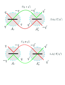
Figure 4: (Color online) Schematic representation of interference terms. In the squared amplitude $\int dq\;dq^{\prime}A(q)A^{\ast}(q^{\prime})$, the part of the amplitude in which both photons undergo reflection at the beam splitter ($A_{r}$) interferes with the portion in which both photons are transmitted at the beam splitter $(A_{t})$. For these terms, $q=-q^{\prime}$, due to the delta function that connects the amplitudes.

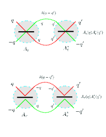
Figure 5: (Color online) Schematic representation of noninterference terms. In the top part of the figure the transmission portion of the amplitude $A_{t}$ interacts only with itself, while in the bottom part the same is true of the reflection amplitude $A_{r}$. For these terms, $q=q^{\prime}$

In contrast, odd-order cancellation occurs when the following combination of ingredients is present:

B1. The Fourier transforming action of the lens, as in A1.

B2. For every photon of transverse momentum ${\mathbf{q}}$ there is a photon of $-{\mathbf{q}}$ present due to downconversion.

B3. $G_{1}=G_{2}$, so that the product $G_{1}\left({{fq}\over k}\right)G_{2}\left(-{{f{\mathbf{q}}}\over k}\right)$ becomes $G_{1}\left({{f{\mathbf{q}}}\over k}\right)G_{1}\left(-{{f{\mathbf{q}}}\over k}\right)=e^{i\left[\phi_{1}({\mathbf{q}})+\phi_{1}(-{\mathbf{q}})\right]}.$ (Note that the cancellation is taking place between different terms of equation (20) than were involved in the cancellation of A3.)

In order to have all-order cancellation, there are two possibilities. Either both of the above sets of conditions may be satisfied simultaneously, or else a third set of conditions may be satisfied:

C1. Same as A1 and B1.

C2. The condition ${\mathbf{q}}={\mathbf{q}^{\prime}}$ must be satisfied, as in the background term $R_{0}$. This occurs in the noninterference terms of figure 5.

C3. Similar to A3, the $G_{j}\left({{f{\mathbf{q}}}\over k}\right)G_{j}^{\ast}\left({{f{\mathbf{q}^{\prime}}}\over k}\right)$ structure arises from the quantum mechanical absolute squaring of the amplitude. But now, coupled with C2, we have $G_{j}\left({{f{\mathbf{q}}}\over k}\right)G_{j}^{\ast}\left({{f{\mathbf{q}}}\over k}\right)=e^{i\left[\phi_{j}({\mathbf{q}})-\phi_{j}({\mathbf{q}})\right]}=1$, giving cancellation of all orders.

In A3 and C3 the phase from a single arm of the interferometer cancels with itself, whereas B3 is a cancellation between the two different (but identical in this case) arms. Cases A and B both involve interference between the amplitudes $A_{r}$ and $A_{t}$ (shown schematically in figure 4), while case C comes from the non-interference terms of figure 5, and so will occur even if only one of the two amplitudes $A_{r}$ and $A_{t}$ is present.

IV Conclusions

To summarize the main results of this paper, for the apparatus of figure 1 we have found that:

$\bullet$ Even-order aberrations induced by the samples $G_{1}$ and $G_{2}$ cancel.

$\bullet$ If the two beams overlap so that $G_{1}=G_{2}$, then all orders of aberration cancel.

$\bullet$ These cancellations only occur if $G_{1}$ and $G_{2}$ are confined to the $z=0$ plane.

These results open up the possibility of using quantum interferometry to eliminate the effects of sample-induced aberration in experiments using temporal correlation-based methods such as dynamical light scattering or fluorescence correlation spectroscopy.

Through the continued study of aberration-cancellation and dispersion-cancellation, it is hoped that a better understanding of the effects of objects or materials placed in an optical system, and better methods of controlling those effects, will gradually emerge. The results reported here are one more step along that path.

The effects described in this paper make essential use of the spatial entanglement (or equivalently the transverse momentum entanglement) between the photons in the downconversion pair. In contrast, the frequency entanglement played no essential role. Similarly, the anticorrelation of the polarizations was used primarily to control the paths of the photons and then to erase the path information; but these functions could be accomplished by other means. So only the spatial entanglement was essential. On the other hand, it is the frequency entanglement that is essential for dispersion cancellation. A question for future investigation is whether use of the simultaneous entanglement of frequency, momentum, and polarization variables (so-called hyperentanglement) may allow control over further optical effects of materials.

- (1) M. Born and E. Wolf, Principles of Optics, 7th edition, Cambridge University Press (1999).
- (2) H.A. Buchdahl, Optical Aberration Coefficients, Dover Publications (1968).
- (3) J.C. Wyant and K. Creath, Basic Wavefront Aberration Theory for Optical Metrology, in Applied Optics and Optical Engineering, Vol. XI, Academic Press (1992).
- (4) C. Bonato, A.V. Sergienko, B.E.A. Saleh, S. Bonora, P. Villoresi, Phys. Rev. Lett. 101 233603 (2008).
- (5) C. Bonato, D.S. Simon, P. Villoresi, A.V. Sergienko, Phys. Rev. A 79 062304 (2009).
- (6) J.D. Franson, Phys. Rev. A 45 3126 (1992).
- (7) A.M. Steinberg, P.G. Kwiat, R.Y. Chiao, Phys. Rev. Lett. 68 2421 (1992).
- (8) B.J. Berne and R. Pecora, Dynamic Light Scattering; with Applications to Chemistry, biology, and Physics, Wiley, New York (1976).
- (9) R. Pecora ed., Dynamic Light Scattering: Applications to Photon Correlation Spectroscopy, Plenum Press, New York, (1985).
- (10) S. Maiti, U. Haupts, W.W. Webb, Proc. Nat.Acad. Sci. USA 94, 11757 (1997).
- (11) M.H. Rubin, D.N. Klyshko, Y.H. Shih, A.V. Sergienko, Phys. Rev. A 50 5122 (1994).
- (12) O. Minaeva, C. Bonato, B.E.A. Saleh, D.S. Simon, A.V. Sergienko, Phys. Rev. Lett. 102 100504 (2009).