Large deviations and ensembles of trajectories in stochastic models

Abstract

We consider ensembles of trajectories associated with large deviations of time-integrated quantities in stochastic models. Motivated by proposals that these ensembles are relevant for physical processes such as shearing and glassy relaxation, we show how they can be generated directly using auxiliary stochastic processes. We illustrate our results using the Glauber-Ising chain, for which biased ensembles of trajectories can exhibit ferromagnetic ordering. We discuss the relation between such biased ensembles and quantum phase transitions.

1 Introduction

This article is concerned with ensembles of trajectories (time-realisations) of stochastic model systems, in which we impose constraints on time-integrated quantities. For example, one might consider an system coupled to two particle reservoirs over a time period $t$, and insist that the total current through the system takes a given value [1]. Such ensembles underlie a range of general results in non-equilibrium systems [2, 3, 8, 4, 5, 6, 7] and have been used to investigate transport properties in simple models and specific non-equilibrium steady states [1, 9]. Recently, they have also been employed in studies of the glass transition [10, 11, 14, 13, 12], where adjusting constraints on such ensembles can drive ergodic ‘model fluids’ into non-ergodic states that resemble ‘ideal glasses’.

The language of ensembles and constraints indicates that our methods will be related to those of equilibrium thermodynamics. The crucial difference is that we consider constraints on time-integrated quantities, while thermodynamics is concerned with constraints that apply at all times in a system. While these definitions may sound similar, they typically lead to quite different behaviour. To understand this difference in a qualitative way, we observe that macrostates in constrained thermodynamic systems may be obtained by minimising the free energy, which corresponds to a minimisation of the work required to introduce the macroscopic constraints. On the other hand, when time-integrated quantities are being constrained, one must instead minimise a ‘dynamical free energy’ that corresponds to the power required to maintain the constraints, in the face of thermal fluctuations [5]. For a constraint on a given quantity, minimising the work and the power are not equivalent: to minimise the dissipated power, it is preferable for the system to enter states from which spontaneous relaxation to equilibrium is very slow, even if the work required to generate such states is relatively large. For example, we show below that in a $1d$ Ising chain, the power required to stabilise low energy states is minimised if the system develops ferromagnetic order, while the work required to attain the same instantaneous value of the energy is minimised by a paramagnetic state – after all, constraining the energy to low values corresponds to considering low temperature, which in $1d$ only ever produces paramagnetic states.

Thus, the ensembles of trajectories that we consider here are not straightforwardly related to thermodynamic ensembles. Nevertheless, studies of the glass transition [10, 11] and of boundary-driven sheared systems [9] have proposed that ensembles of trajectories generated in this way are relevant for the results of physical experiments. Establishing a connection between constrained ensembles of trajectories and experimental systems is a complicated task. For example, the most natural representation of the constrained ensemble does not have a Markov form for the transition rates. Further, causality may be broken, in the sense that applying a perturbation at time $t_{\mathrm{w}}$ may incur a response at times $t<t_{\mathrm{w}}$. Here, we describe some general features of such constrained ensembles of trajectories, aiming to understand what physical protocol might lead to the same behaviour as a constraint on a time-averaged quantity.

Our results are organised into two sections. In Section 2, we review some general aspects of the large deviation formalism that we will use, and we define an ‘auxiliary model’ that is a Markov stochastic process whose steady state trajectories are close to those of the constrained ensembles (in a sense discussed below). A similar result was described by Evans [9]: we show how the rules discussed in that work can be derived through a similarity transformation between master operators for stochastic processes. For cases where the constrained ensemble of trajectories is time-reversal invariant, the auxiliary model can be obtained though a modification of the energy function for the original model. We discuss the extent to which these auxiliary models represent physical realisations of the constrained ensembles described above. Then, in Section 3, we investigate spontaneous breaking of ergodicity in constrained ensembles of trajectories, for the (one-dimensional) Glauber-Ising chain. Despite its $1d$ nature, constraining ensembles of trajectories in this model may induce long-ranged order and spontaneous symmetry breaking. The mechanism is identical to that behind quantum phase transitions, where real time in the stochastic model plays the role of imaginary time in a path integral representation of the density matrix. We discuss the interpretation of the auxiliary stochastic model in this context.

2 Biased ensembles of trajectories

2.1 Definitions

We consider stochastic models in continuous time. A model is defined through a (discrete) set of configurations $\{\mathcal{C}_{1},\mathcal{C}_{2},\dots\}$ and stochastic transition rates $W(\mathcal{C}^{\prime}\to\mathcal{C})$. Then, if $p(\mathcal{C},t)$ is the probability of finding the system in configuration $\mathcal{C}$ at time $t$, the master equation of the model is

$$\frac{\partial}{\partial t}p(\mathcal{C},t)=-r(\mathcal{C})p(\mathcal{C},t)+\sum_{\mathcal{C}^{\prime}\neq\mathcal{C}}W(\mathcal{C}^{\prime}\to\mathcal{C})p(\mathcal{C}^{\prime},t)$$ (1)

where $r(\mathcal{C})=\sum_{\mathcal{C}^{\prime}\neq\mathcal{C}}W(\mathcal{C}\to\mathcal{C}^{\prime})$ is the escape rate from configuration $\mathcal{C}$. Writing $|P(t)\rangle=\sum_{\mathcal{C}}p(\mathcal{C},t)|\mathcal{C}\rangle$, the master equation can be written as $\frac{\partial}{\partial t}|P(t)\rangle=\mathbb{W}|P(t)\rangle$ where the matrix elements of the operator $\mathbb{W}$ are simply $\langle\mathcal{C}|\mathbb{W}|\mathcal{C}^{\prime}\rangle=W(\mathcal{C}^{\prime}\to\mathcal{C})-\delta_{\mathcal{C},\mathcal{C}^{\prime}}r(\mathcal{C})$.

We consider large deviations of time-integrated quantities of the form

$$\mathcal{B}_{t}=\int_{0}^{t}\!\mathrm{d}t^{\prime}B(t^{\prime})$$ (2)

where $B(t)$ is an observable that depends only the configuration of the system at time $t$. (In Section 3, we will take $B(t)$ to be simply the energy of the system.) Alternatively, one can consider large deviations fluxes or dynamical activities. That is, assume that an observable $\mathcal{A}_{t}$ acquires contributions whenever the system changes configuration: if the sequence of configurations in a trajectory is $\mathcal{C}_{0},\mathcal{C}_{1},\dots,\mathcal{C}_{K}$ then $\mathcal{A}_{t}$ can be written in the form

$$\mathcal{A}_{t}=\sum_{k=0}^{K-1}\alpha(\mathcal{C}_{k},\mathcal{C}_{k+1}).$$ (3)

For example, one might take $\alpha(\mathcal{C}_{k},\mathcal{C}_{k+1})=1$ for all pairs of distinct configurations, so that $\mathcal{A}_{t}$ counts the number of configuration changes between time $0$ and time $t$ [10, 11]. Alternatively, one might take $\alpha(\mathcal{C}_{k},\mathcal{C}_{k+1})$ to be the contribution of the stochastic transition $\mathcal{C}_{k}\to\mathcal{C}_{k+1}$ to a total current [1], accumulated shear [9], entropy current [6], or dynamical entropy [15]. For convenience, we concentrate on observables of the form $\mathcal{B}_{t}$, but most of our results generalise straightforwardly[14, 15] to time-extensive observables of the form $\mathcal{A}_{t}$.

Following the discussion in the introduction, we are interested in ensembles of trajectories where $\mathcal{B}_{t}$ is constrained to be far from its average value $\langle\mathcal{B}_{t}\rangle_{0}$, where $\langle\cdot\rangle_{0}$ indicates an average in the steady state of the stochastic model. However, it is convenient to exploit an equivalence of ensembles in the spirit of microcanonical/canonical equivalence in statistical mechanics: instead of a constrained ensemble, we define a ‘biased ensemble’ by assigning to each trajectory $\pi$ a probability that depends on a ‘biasing field’ $g$:

$$P[\pi,g]=Z(g,t)^{-1}P[\pi,0]\exp\left[-g\mathcal{B}_{t}\right]$$ (4)

where $P[\pi,0]$ is the probability of observing trajectory $\pi$ in the (unbiased) steady state of the stochastic model and

$$Z(g,t)=\left\langle\exp\left[-g\mathcal{B}_{t}\right]\right\rangle_{0}$$ (5)

is the partition function for the new ensemble. Our formalism and notation closely follows Ref. juanpe-fred-jpa, and we refer to that paper for further technical details. We note that the field $g$ was denoted by $s$ in Refs. s-glass, juanpe-fred-jpa,p2-paper,rom-paper, and the resulting biased ensembles accordingly referred to as $s$-ensembles. We prefer $g$ in this article to avoid confusion with Ising spins $s_{i}$ in later sections. Averages within the biased ensemble are given by

$$\langle O\rangle_{g}=Z(g,t)^{-1}\left\langle O\exp\left[-g\mathcal{B}_{t}\right]\right\rangle_{0}$$ (6)

where $O$ may be any trajectory-dependent observable, and the average depends implicitly on the time $t$ as well as on $g$.

From a mathematical point of view, one may identify $Z(g,t)$ as the generating function for the moments of $\mathcal{B}_{t}$. Physically, we note that the effect of $g$ is to bias the average $\langle\mathcal{B}_{t}\rangle_{g}$. Then, we appeal to equivalence of ensembles: the ensemble defined by (4) is equivalent to an ensemble in which $\mathcal{B}_{t}$ is constrained to take the value $\langle\mathcal{B}_{t}\rangle_{g}$, where equivalence holds in the same sense as for the canonical and microcanonical ensembles in statistical mechanics.

Finally, we obtain the ‘dynamical free energy’ of the biased ensemble. Let $p^{\mathrm{ss}}(\mathcal{C})$ be the probability of observing configuration $\mathcal{C}$ in the (unbiased) steady state of the original model. Then, one may write [15]

$$Z(g,t)=\langle e|\mathrm{e}^{\mathbb{W}(g)t}|\mathrm{ss}\rangle$$ (7)

where $\langle e|=\sum_{\mathcal{C}}\langle\mathcal{C}|$ is a projection state, $|\mathrm{ss}\rangle=\sum_{\mathcal{C}}p^{\mathrm{ss}}(\mathcal{C})|\mathcal{C}\rangle$, and

$$\mathbb{W}(g)=\mathbb{W}-g\sum_{\mathcal{C}}|\mathcal{C}\rangle\langle\mathcal{C}|b(\mathcal{C})$$ (8)

where $b(\mathcal{C})$ is the value of the observable $B$ in configuration $\mathcal{C}$. Assuming for convenience that the original stochastic model is irreducible and has a finite state space, one makes a spectral decomposition of $\mathbb{W}(g)=\sum_{i}|V_{i}\rangle\omega_{i}\langle U_{i}|$, and it follows from (7) that the dynamical free energy is [6, 15]

$$\psi(g)\equiv-\lim_{t\to\infty}t^{-1}\log Z(g,t)=-\max_{i}\omega_{i}.$$ (9)

We note that while we assumed an irreducible model and a finite system, these are not necessary for (9) to hold. However, infinite systems with spontaneously broken ergodicity [16, 13] or absorbing states [17] require some additional assumptions on the operator $\mathbb{W}(g)$.

If we wish to consider the large deviations of observables $\mathcal{A}_{t}$ defined as in (3), the analysis is very similar: Equs. (4)-(9) still hold, with $\mathcal{B}_{t}$ simply replaced by $\mathcal{A}_{t}$. However, the operator $\mathbb{W}(g)$ has a different form in this case [15, 14]: its matrix elements are

$$\langle\mathcal{C}|\mathbb{W}(g)|\mathcal{C}^{\prime}\rangle=\left\{\begin{array}[]{ll}W(\mathcal{C}^{\prime}\to\mathcal{C})\mathrm{e}^{-g\alpha(\mathcal{C}^{\prime},\mathcal{C})},&\mathcal{C}\neq\mathcal{C}^{\prime},\\ -r(\mathcal{C}),&\mathcal{C}=\mathcal{C}^{\prime}.\end{array}\right.$$ (10)

2.2 Time-translational invariance, and an auxiliary stochastic process that generates the biased ensemble

We now turn to physical features of the biased ensemble of (4). Averages $\langle O\rangle_{0}$ in the steady state of the stochastic model are clearly time-translational invariant. However, this invariance is broken for observables such as $\langle O\rangle_{g}$. For example, if one takes a configuration-dependent observable $F$, averages such as $\langle F(t^{\prime})\rangle_{g}$ may depend on $t^{\prime}$ since the bias in (4) breaks time-translation invariance (TTI). However, as long as the operator $\mathbb{W}(g)$ is not at a critical point (in a sense defined below), we have

$$\langle F(t^{\prime})\rangle_{g}=\left\{\begin{array}[]{ll}F_{\infty},&\tau\ll t^{\prime},\ \tau\ll t-t^{\prime}\\ F_{\mathrm{f}}&t^{\prime}=t\gg\tau\end{array}\right.$$ (13)

where $\tau$ is a relaxation time into the TTI regime, discussed below. In general, the biased ensembles are TTI for a range of times $t^{\prime}$ such that $\tau\ll t^{\prime}$ and $\tau\ll t-t^{\prime}$.

To understand the TTI regime in more detail, we consider the operator $\mathbb{W}(g)$. This operator is not Hermitian, so it has separate left and right eigenvectors associated with its largest eigenvalue, which we denote by $\langle U|=\sum_{\mathcal{C}}\langle\mathcal{C}|u(\mathcal{C})$ and $|V\rangle=\sum_{\mathcal{C}}v(\mathcal{C})|\mathcal{C}\rangle$ respectively. (We normalise such that $\langle e|V\rangle=1=\langle U|V\rangle$. This is possible since the $u(\mathcal{C})$ and $v(\mathcal{C})$ are non-negative, as will become clear from the probability interpretation derived below.) Then, for long times $t^{\prime}$, we have

$$\mathrm{e}^{\mathbb{W}(g)t^{\prime}}=\mathrm{e}^{-\psi(g)t^{\prime}}\left[|V\rangle\langle U|+\mathcal{O}(\mathrm{e}^{-\Delta\omega t^{\prime}})\right],$$ (14)

where $\Delta\omega$ is the difference between the largest and second-largest eigenvalues of $\mathbb{W}(g)$. If we restrict to irreducible stochastic models with finite state spaces then $\Delta\omega>0$ and we identify $\tau=(\Delta\omega)^{-1}$. However, in the limit of large system size, $\Delta\omega$ may vanish. In some cases, this signifies a critical point for the operator $\mathbb{W}(g)$, while in other cases, the analysis of this section may be generalised and the TTI regime still exists. Examples of both cases are discussed in Section 3.

In any case, one has from (13) that

$$F_{\infty} = \lim_{t\to\infty}\langle e|\mathrm{e}^{\mathbb{W}(g)(t-t^{\prime})}\hat{F}\mathrm{e}^{\mathbb{W}(g)t^{\prime}}|\mathrm{ss}\rangle Z(g,t)^{-1}$$ (15)

$$F_{\mathrm{f}} = \lim_{t\to\infty}\langle e|\hat{F}\mathrm{e}^{\mathbb{W}(g)t}|\mathrm{ss}\rangle Z(g,t)^{-1}$$ (16)

where $\hat{F}=\sum_{\mathcal{C}}|\mathcal{C}\rangle\langle\mathcal{C}|f(\mathcal{C})$, with $f(\mathcal{C})$ being the value of observable $F$ in configuration $\mathcal{C}$. Then, as long as the corrections in (14) are small, one has $Z(g,t)=\mathrm{e}^{-\psi(g)t}\langle U|\mathrm{ss}\rangle$ and so

$$F_{\infty}=\langle U|\hat{F}|V\rangle=\sum_{\mathcal{C}}f(\mathcal{C})u(\mathcal{C})v(\mathcal{C}),\qquad F_{\mathrm{f}}=\langle e|\hat{F}|V\rangle=\sum_{\mathcal{C}}f(\mathcal{C})v(\mathcal{C})$$ (17)

Taking then $F$ to be simply an indicator function for configuration $\mathcal{C}$, one sees that the probability of observing this configuration in the TTI regime of the biased ensemble is

$$p^{\mathrm{TTI}}(\mathcal{C})=u(\mathcal{C})v(\mathcal{C}),$$ (18)

while the probability of observing the same configuration at the final time $t$ is simply $v(\mathcal{C})$. Indeed, as $t^{\prime}$ is reduced from $t$, $\langle F(t^{\prime})\rangle_{g}$ decays exponentially from $F_{\mathrm{f}}$ to $F_{\infty}$, on a time scale $\tau=(\Delta\omega)^{-1}$.

We now construct an auxiliary stochastic model whose (unbiased) trajectories coincide with those of the biased ensemble of (4), within the TTI regime. We will show that, in terms of the diagonal operator $\hat{U}=\sum_{\mathcal{C}}|\mathcal{C}\rangle\langle\mathcal{C}|u(\mathcal{C})$, the master operator of this auxiliary model is

$$\mathbb{W}^{\mathrm{aux}}=\hat{U}\mathbb{W}(g)\hat{U}^{-1}+\psi(g).$$ (19)

The off-diagonal matrix elements of this operator must then be the transition rates between the configurations of the system. For biased ensembles defined as in (4), these rates are

$$W^{\mathrm{aux}}(\mathcal{C}^{\prime}\to\mathcal{C})\equiv\langle\mathcal{C}|\mathbb{W}^{\mathrm{aux}}|\mathcal{C}^{\prime}\rangle=u(\mathcal{C})W(\mathcal{C}^{\prime}\to\mathcal{C})\frac{1}{u(\mathcal{C}^{\prime})},$$ (20)

which are non-negative as they should be. The model is also stochastic: $\sum_{\mathcal{C}}\langle\mathcal{C}|\mathbb{W}^{\mathrm{aux}}=\langle e|\mathbb{W}^{\mathrm{aux}}=0$ which follows since $\langle U|=\langle e|\hat{U}$ is a left eigenvector of $\mathbb{W}(g)$ with eigenvalue $-\psi(g)$. Thus, the diagonal elements of $\mathbb{W}^{\mathrm{aux}}$ are simply $\langle\mathcal{C}|\mathbb{W}^{\mathrm{aux}}|\mathcal{C}\rangle=-\sum_{\mathcal{C}^{\prime}}W^{\mathrm{aux}}(\mathcal{C}\to\mathcal{C}^{\prime})$.

Two comments are in order. Firstly, if the bias in (4) uses an observable $\mathcal{A}_{t}$ in place of $\mathcal{B}_{t}$, the auxiliary rates are modified to

$$W^{\mathrm{aux}}(\mathcal{C}^{\prime}\to\mathcal{C})\equiv\langle\mathcal{C}|\mathbb{W}^{\mathrm{aux}}|\mathcal{C}^{\prime}\rangle=u(\mathcal{C})W(\mathcal{C}^{\prime}\to\mathcal{C})\mathrm{e}^{-g\alpha(\mathcal{C}^{\prime},\mathcal{C})}\frac{1}{u(\mathcal{C}^{\prime})}.$$ (21)

Secondly, applying this generalised result to an ensemble biased by the total shear, one obtains the result of Evans [9]: we identify our $u(\mathcal{C})$ with his $\mathrm{e}^{q_{\mathcal{C}}}$, where $q_{\mathcal{C}}$ is defined as a measure of “the propensity [of configuration $\mathcal{C}$] to exhibit flux in the future”, via $\mathrm{e}^{q_{\mathcal{C}}}=\lim_{t^{\prime}\to\infty}\frac{1}{Z(t^{\prime})}\sum_{\mathcal{C}^{\prime}}\langle\mathcal{C}^{\prime}|\mathrm{e}^{\mathbb{W}(g)t^{\prime}}|\mathcal{C}\rangle=u(\mathcal{C})/\langle U|\mathrm{ss}\rangle\propto u(\mathcal{C})$.

We also note that $|\mathrm{TTI}\rangle=\sum_{\mathcal{C}}p^{\mathrm{TTI}}(\mathcal{C})|\mathcal{C}\rangle$ is a right eigenvector of $\mathbb{W}^{\mathrm{aux}}$ with eigenvalue zero, and we identify this as the steady state distribution of the auxiliary model, consistent with our assertion that the steady state trajectories of the auxiliary model are those of the biased ensemble of (4) in the TTI regime.

To demonstrate that the auxiliary model is valid, we now need to show that this correspondence holds for all trajectories and not simply for the steady state distribution over configurations. Consider, then, the probability that a given path occurs within the TTI regime of the biased ensemble. We define the path $\pi$ by discretising time in the manner of a path integral. That is, we state the configuration of the system at a sequence of equally-spaced times: taking the spacing $\Delta t$ to zero then allows us to specify the path with arbitrary precision. Let the sequence of configurations be $\mathcal{C}_{0},\mathcal{C}_{1},\dots,\mathcal{C}_{M}$, where $\mathcal{C}_{0}$ occurs at a time $t_{0}$ so that $\mathcal{C}_{M}$ occurs at time $t_{0}+M\Delta t$. To ensure that we are in the TTI regime we take $\tau\ll t_{0}$ and $\tau\ll t-(t_{0}+M\Delta t)$. Then, the probability of the path $\pi$ in the biased ensemble is simply

$$P[\pi,g]=\left[\sum_{\mathcal{C}}G_{\mathcal{C},\mathcal{C}_{M}}(t-t_{0}-M\Delta t)\right]\left[\prod_{i=1}^{M}G_{\mathcal{C}_{i},\mathcal{C}_{i-1}}(\Delta t)\right]\sum_{\mathcal{C}}G_{\mathcal{C}_{0},\mathcal{C}}(t_{0})p^{\mathrm{ss}}(\mathcal{C})\frac{1}{Z(g,t)}$$ (22)

where $G_{\mathcal{C},\mathcal{C}^{\prime}}(t^{\prime})=\langle\mathcal{C}|\mathrm{e}^{\mathbb{W}(g)t^{\prime}}|\mathcal{C}^{\prime}\rangle$ is akin to a propagator in the biased ensemble and $p^{\mathrm{ss}}(\mathcal{C})$ was defined above to be the probability of observing configuration $\mathcal{C}$ in the (unbiased) steady state of the original model. We emphasise that this representation of the path-probability does not correspond directly to a Markov chain since $G_{\mathcal{C},\mathcal{C}^{\prime}}(t^{\prime})$ is not a stochastic matrix [$\sum_{\mathcal{C}}G_{\mathcal{C},\mathcal{C}^{\prime}}\neq 1$ because $\mathbb{W}(g)$ is not a stochastic master operator].

Then, within the TTI regime of the biased ensemble, we have from (14) that

$$P[\pi,g]\approx u(\mathcal{C}_{M})\left[\prod_{i=1}^{M}G_{\mathcal{C}_{i},\mathcal{C}_{i-1}}(\Delta t)\right]v(\mathcal{C}_{0})\frac{1}{\mathrm{e}^{-\psi(g)M\Delta t}}$$ (23)

where the approximate equality is exact in the TTI regime, with the exponentially small corrections given in (14). Finally, we define the propagator of the auxiliary model, and using the definition of $\mathbb{W}^{\mathrm{aux}}$, we have

$$G^{\mathrm{aux}}_{\mathcal{C},\mathcal{C}^{\prime}}(t^{\prime})\equiv\langle\mathcal{C}|\mathrm{e}^{\mathbb{W}^{\mathrm{aux}}(g)t^{\prime}}|\mathcal{C}^{\prime}\rangle=u(\mathcal{C})G_{\mathcal{C},\mathcal{C}^{\prime}}(t^{\prime})\frac{1}{u(\mathcal{C}^{\prime})}\mathrm{e}^{\psi(g)t^{\prime}}$$ (24)

This represents a stochastic propagator, in the sense that $\sum_{\mathcal{C}}G^{\mathrm{aux}}_{\mathcal{C},\mathcal{C}^{\prime}}(t)=1$. Thus, the path probability in the biased ensemble is

$$P[\pi,g]\approx\left[\prod_{i=1}^{M}G^{\mathrm{aux}}_{\mathcal{C}_{i},\mathcal{C}_{i-1}}(\Delta t)\right]p^{\mathrm{TTI}}(\mathcal{C}_{0})$$ (25)

where the approximate equality is exact in the TTI regime, as above. We recognise the right hand side of (25) as the path probability for the (stochastic) auxiliary model in its steady state.

Thus, we have shown that the steady state associated with the biased ensemble of trajectories can be interpreted as the steady state of an auxiliary stochastic model that is Markov and TTI. Transition rates that are non-zero in the original model are also non-zero in the auxiliary model, and vice versa. (For example, if the original model has only single spin flip moves then so does the auxiliary model, and if some moves are forbidden by kinetic constraints in the original model [18, 11] then these constraints are preserved in the auxiliary model.) However, we note that the auxiliary model may be unphysical in the sense that the dynamical rules are non-local. For example, in stochastic spin models the rate for flipping a given spin typically depends only on the states of that spin and of a few spins in its neighbourhood. Even if the original model $\mathbb{W}$ is constructed in this way, the auxiliary model $\mathbb{W}^{\mathrm{aux}}$ typically does not share this feature. In general, it is not clear if such non-local interactions render these biased ensembles unphysical, or if they might arise from non-trivial fluctuation forces in non-equilibrium states, as proposed by Evans [9].

We end this section with a note about causality: if we consider an unbiased ensemble of trajectories that begins at equilibrium but is perturbed (by a change in its transition rates) at some time $t_{\mathrm{w}}$, then the response to the perturbation is zero for all times $t^{\prime}<t_{\mathrm{w}}$. However, if we then use these perturbed trajectories to generate a biased ensemble as in (4), then one will generically observe a response to the perturbation for times $t^{\prime}<t_{\mathrm{w}}$. This is the violation of causality that was mentioned in the introduction. Clearly then, a perturbation to the original transition rates at time $t_{\mathrm{w}}$ cannot be taken into account through a perturbation at time $t_{\mathrm{w}}$ in the auxiliary model.

2.3 Time-reversal invariance and a variational result

So far, we have considered a general stochastic model. We now focus on ensembles of trajectories that are time-reversal invariant. For the unbiased ensemble of trajectories, this condition is met for stochastic models obeying detailed balance: $W(\mathcal{C}\to\mathcal{C}^{\prime})\mathrm{e}^{-\beta E(\mathcal{C})}=W(\mathcal{C}^{\prime}\to\mathcal{C})\mathrm{e}^{-\beta E(\mathcal{C}^{\prime})}$ where $E(\mathcal{C})$ is the energy of configuration $\mathcal{C}$, and $\beta$ is the inverse temperature, as above. In this case, biased ensembles of trajectories defined as in (4) are also time-reversal invariant, and the operator $\mathbb{W}(g)$ may be symmetrised by a similarity transformation:

$$\mathbb{H}(g)=\mathrm{e}^{\beta\hat{E}/2}\mathbb{W}(g)\mathrm{e}^{-\beta\hat{E}/2}$$ (26)

where $\hat{E}$ is the (diagonal) energy operator. Such a symmetrisation is possible because the bias introduced in (4) is itself time-reversal symmetric. One may also consider biasing ensembles according to observables $\mathcal{A}_{t}$ defined as in (3). In this case, if the unbiased model obeys detailed balance then the biased ensemble is time-reversal symmetric only if the bias is also time-reversal symmetric: $\alpha(\mathcal{C},\mathcal{C}^{\prime})=\alpha(\mathcal{C}^{\prime},\mathcal{C})$. An example is the case where $\mathcal{A}_{t}$ is simply the number of configuration changes in the trajectory, with $\alpha(\mathcal{C},\mathcal{C}^{\prime})=1$ for all pairs of distinct configurations. However, if $\mathcal{A}_{t}$ is a current or a flux then time-reversal symmetry is typically broken, and $\mathbb{W}(g)$ may not be symmetrised.

We also note that if the rates $W(\mathcal{C}\to\mathcal{C}^{\prime})$ obey detailed balance then so do the rates of the auxiliary model. Since $\mathbb{H}(g)$ is symmetric, the left and right eigenvectors of $\mathbb{W}(g)$ are related through $v(\mathcal{C})=u(\mathcal{C})\mathrm{e}^{-\beta E(\mathcal{C})}$. Expressing $\mathbb{H}(g)$ in terms of $\mathbb{W}^{\mathrm{aux}}$ and multiplying it from both sides first by $\mathrm{e}^{-\beta\hat{E}/2}$ and then by $\hat{U}$ also shows that $\mathbb{W}^{\mathrm{aux}}\hat{U}\mathrm{e}^{-\beta\hat{E}}\hat{U}$ is symmetric, i.e.

$$W^{\mathrm{aux}}(\mathcal{C}^{\prime}\to\mathcal{C})u(\mathcal{C}^{\prime})v(\mathcal{C}^{\prime})=W^{\mathrm{aux}}(\mathcal{C}\to\mathcal{C}^{\prime})u(\mathcal{C})v(\mathcal{C})$$ (27)

Thus, the auxiliary rates $W^{\mathrm{aux}}(\mathcal{C}\to\mathcal{C}^{\prime})$ obey detailed balance with respect to the steady state distribution $p^{\mathrm{TTI}}(\mathcal{C})$ defined above, as claimed. We therefore define an auxiliary energy function $E^{\mathrm{aux}}$ through

$$\mathrm{e}^{-\beta E^{\mathrm{aux}}(\mathcal{C})}=u(\mathcal{C})v(\mathcal{C})=\mathrm{e}^{-\beta E(\mathcal{C})}u(\mathcal{C})^{2}$$ (28)

so that the difference in the energy of a configuration between unbiased and auxiliary models is $E^{\mathrm{aux}}(\mathcal{C})-E(\mathcal{C})=(-2/\beta)\ln u(\mathcal{C})$.

We emphasise that the transition rates in the auxiliary model can be obtained from the rates of the original model using only the auxiliary energy function as additional information. Further, since the operator $\mathbb{H}(g)$ is symmetric, one may obtain the dynamical free energy through a variational principle

$$-\psi(g)=\max_{|\phi\rangle}\frac{\langle\phi|\mathbb{H}(g)|\phi\rangle}{\langle\phi|\phi\rangle}$$ (29)

with equality when $|\phi\rangle=\sum_{\mathcal{C}}\sqrt{u(\mathcal{C})v(\mathcal{C})}|\mathcal{C}\rangle$. This may be interpreted as an extremisation over variational estimates for the steady state distribution through $|\phi\rangle=\sum_{\mathcal{C}}\sqrt{p^{\mathrm{var}}(\mathcal{C})}|\mathcal{C}\rangle$, with equality when $p^{\mathrm{var}}(\mathcal{C})=p^{\mathrm{TTI}}(\mathcal{C})$. Equivalently, one may consider an extremisation over energy functions $|\phi\rangle=\sum_{\mathcal{C}}\mathrm{e}^{-\beta E^{\mathrm{var}}(\mathcal{C})/2}|\mathcal{C}\rangle$ with equality when $E^{\mathrm{var}}(\mathcal{C})=E^{\mathrm{aux}}(\mathcal{C})$. However, as noted above, models with short-ranged interactions have energy functions consisting of sums over local contributions, but there is no reason to suppose that $E^{\mathrm{aux}}(\mathcal{C})$ can be written in this way. A specific example will be given in the next section.

3 $1d$ Glauber-Ising chain, and link with quantum-Ising chain

To illustrate the general features described above, we consider the $1d$ Glauber-Ising chain. We take a periodic chain of $N$ Ising spins, $s_{i}=\pm 1$ with an energy function $E=-\frac{1}{2}\sum_{i}s_{i}s_{i+1}$. Spins flip with Glauber rates, respecting detailed balance: the rate for flipping spin $i$ is $W_{i}=[1+\exp(h_{i}s_{i})]^{-1}$ where $h_{i}=\beta(s_{i-1}+s_{i+1})$. It will also be useful to define domain wall variables $n_{i+\frac{1}{2}}=\frac{1}{2}(1-s_{i}s_{i+1})$, so that $n_{i+\frac{1}{2}}=1$ if there is a domain wall between sites $i$ and $i+1$ while $n_{i+\frac{1}{2}}=0$ otherwise. Periodic boundaries ensure that the total number of domain walls in the system is even, while we note that every configuration of the domain walls corresponds to two different configurations of the spins, related by flipping all of the spins at once. In terms of the domain wall variables, the energy is simply $E=\sum_{i}(n_{i+\frac{1}{2}}-\frac{1}{2})$.

3.1 Large deviations of the energy and a dynamical phase transition

Starting from the Glauber-Ising chain, we define a biased ensemble of trajectories as in (4), taking the observable $B(t)$ to be the energy $E(t)$. We write the master equation in terms of domain-wall variables, respresenting states by associating a spin-half degree of freedom with each bond on the chain. Thus, a domain wall on bond $i+\frac{1}{2}$ corresponds to an up spin, while bonds with $n_{i+\frac{1}{2}}=0$ correspond to down spins. Then, the operator (8) for the biased ensemble has a representation in terms of Pauli matrices $\sigma^{x}_{i+\frac{1}{2}},\sigma^{y}_{i+\frac{1}{2}},\sigma^{z}_{i+\frac{1}{2}}$:

$$\mathbb{W}(g) =\frac{1}{2}\sum_{i}\Big{[} \sigma^{+}_{i-\frac{1}{2}}\sigma^{-}_{i+\frac{1}{2}}+\sigma^{+}_{i-\frac{1}{2}}\sigma^{-}_{i+\frac{1}{2}}+\gamma\sigma^{-}_{i-\frac{1}{2}}\sigma^{-}_{i+\frac{1}{2}}+\lambda\sigma^{+}_{i-\frac{1}{2}}\sigma^{+}_{i+\frac{1}{2}}$$ (30)

$$+(\lambda-1-g)\sigma^{z}_{i+\frac{1}{2}}-1\Big{]}$$

with $\sigma^{\pm}_{i+\frac{1}{2}}=\frac{1}{2}(\sigma_{i+\frac{1}{2}}^{x}\pm\mathrm{i}\sigma_{i+\frac{1}{2}}^{y})$ as usual, $\gamma=2/(1+\mathrm{e}^{-2\beta})$ and $\lambda=2-\gamma=2/(1+\mathrm{e}^{2\beta})$. We note that large deviations of the energy in a similar model with an antiferromagnetic interaction potential may be obtained by taking $\beta<0$ and flipping the sign of $g$ (since $E=+\frac{1}{2}\sum_{i}s_{i}s_{i+1}$ in that case). Symmetrising $\mathbb{W}(g)$ as in (26), one may diagonalise $\mathbb{H}(g)$ using a Jordan-Wigner transformation (as, for example, in section 4.2 of Ref. SachdevQPT, leading to

$$\mathbb{H}(g)=\sum_{k}\left[\Omega_{k}(c_{k}c^{\dagger}_{k}-c^{\dagger}_{k}c_{k})-\frac{1}{2}\right]$$ (31)

where $c^{\dagger}$ and $c$ are fermionic creation and annihilation operators, labelled by a wave vector $k=2m\pi/N$, the sum runs over integer $m$ in the first Brillouin zone, $-\frac{N}{2}<m\leq\frac{N}{2}$, and

$$\Omega_{k}=\sqrt{(g-\lambda+1-\cos k)^{2}+\lambda\gamma\sin^{2}k}.$$ (32)

We have $\Omega_{k}\geq 0$ so that the largest eigenvalue of $\mathbb{H}$ is $-\psi(g)=\sum_{k}(\Omega_{k}-\frac{1}{2})$. The fermion vacuum state has such an eigenvalue, and we identify the difference between the largest and next-largest eigenvalues as $\Delta\omega=\min_{k}(2\Omega_{k})$. Finally, taking the limit of large system size,

$$\psi(g)=\frac{N}{2}\int_{-\pi}^{\pi}\frac{\mathrm{d}k}{2\pi}(1-2\Omega_{k})$$ (33)

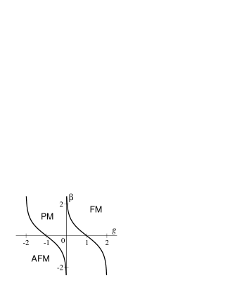
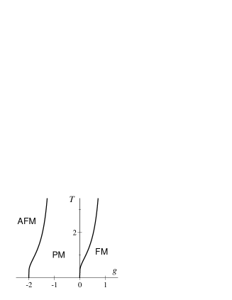
Figure 1: Dynamical phase diagram for the 1d Glauber-Ising chain, as a function of biasing parameter $g$. Solid lines correspond to second-order (critical) phase transitions. (Left) We show the behaviour as a function of inverse temperature $\beta$: the regime with $\beta<0$ corresponds to an antiferromagnetic chain, while $\beta=0$ is the chain at infinite temperature. The equilibrium steady state corresponds to $g=0$ and is always paramagnetic (PM). Large positive $g$ drives the system into a ferromagnetic (FM) phase while large negative $g$ leads to an antiferromagnetic (AFM) phase. On the right, we show the same figure as a function of temperature, to emphasise that both transitions persist all the way to $T=0$. However, the nature of the critical points changes at $T=0$ since the system is no longer time-reversal symmetric.

As well as the dynamical free energy $\psi(g)$, we emphasise that we have obtained the full spectrum of the operator $\mathbb{W}(g)$. A particularly important case for large system sizes is obtained when $\min_{k}\Omega_{k}=0$, so that there are eigenvalues of $\mathbb{W}(g)$ that are arbitrarily close to its maximal eigenvalue $-\psi(g)$. The essential point here is that $\Omega_{k}>0$ except in certain special cases: (i) when $k=0$ and $g=\lambda$, (ii) when $k=\pi$ and $g=-\gamma$ (recall $\gamma+\lambda=2$) and (iii) when $\lambda=0$ is equal to zero and $\cos k=1+g$ (or $\gamma=0$ and $\cos k=g-1$). Case (iii) corresponds to the zero-temperature dynamics of the Ising model, which we do not consider in this work. However, we will consider the cases $g=\gamma>0$ and $g=-\lambda<0$, for which the system becomes critical. It may be verified that the second derivative of $\psi(g)$ diverges at these critical points (note that we have taken this derivative after the limit of large $N$). This divergence signals a (continuous) phase transition in the space of trajectories. In particular, (14) breaks down, and the existence of the TTI regime described in Section 2.2 is no longer assured (this point will be discussed further in Sec. 3.3 below).

Now, the $1d$ Ising model clearly has no phase transition at any finite temperature, so the equilibrium ensembles of trajectories with $g=0$ are those of ergodic paramagnets. However, for $g>\lambda$, the biased ensembles of trajectories are dominated by ferromagnetic configurations: the system acquires long-ranged order in space, and it also breaks ergodicity, exhibiting long-ranged order in time. A similar effect occurs for $g<-\gamma$, for which the system enters an antiferromagnetic state. The ‘dynamical phase diagram’ for this system is shown in Fig. 1. Similar critical phase transitions in biased ensembles have been found in higher-dimensional ferromagnets, for temperatures above their critical points [12, 15]. However, to explain how the physical conclusions described in this section can be drawn directly from the form of $W(g)$, we now show that biased ensembles of trajectories in the $1d$ Ising chain have already been studied extensively in the context of quantum phase transitions [19]. This allows us to identify the universality class of the (continuous) phase transitions at $g=\gamma$ and $g=-\lambda$: as long as we take $T>0$ in the stochastic model, this is the universality class of the (classical) $2d$ Ising model.

3.2 Link with quantum Ising model in a transverse field and hence with the $2d$ Ising model

We begin by taking $\beta=0$ in the original Ising chain, corresponding to infinite temperature, so that all single spin-flip transitions take place with rate $\frac{1}{2}$. In this case, we have, using the superscript ($n$) to emphasize that we are in the domain wall basis,

$$\mathbb{H}^{(n)}(g)=\mathbb{W}^{(n)}(g)=\frac{1}{2}\sum_{i}\left[\sigma^{x}_{i+\frac{1}{2}}\sigma^{x}_{i-\frac{1}{2}}-1-g\sigma^{z}_{i+\frac{1}{2}}\right]$$ (34)

One may also work in the spin basis, using a spin-half degree of freedom for each of the original Ising spins: for $\beta=0$, one has a master operator

$$\mathbb{H}^{(s)}(g)=\mathbb{W}^{(s)}(g)=\frac{1}{2}\sum_{i}\left[\sigma^{x}_{i}-1+g\sigma^{z}_{i}\sigma^{z}_{i+1}\right]$$ (35)

These operators are familiar from studies of quantum spin chains. To be precise, $[-\mathbb{H}^{(s)}(g)]$ is the Hamiltonian for an Ising ferromagnet in transverse field, a canonical model for quantum phase transitions (QPTs) [19]. In $[-\mathbb{H}^{(s)}(g)]$, one identifies $g$ as an Ising coupling between spins, while the term proportional to $\sigma^{x}$ is a ‘transverse field’ that frustrates ferromagnetic ordering. As $g$ is tuned through $g=1$, the ground state energy $\psi(g)$ has a singularity, and the system acquires long-ranged ferromagnetic order. The point $g=1$ is critical in that it exhibits a diverging correlation length [19]. Representing the partition function for the quantum system as an imaginary time path integral, one sums over an ensemble of periodic trajectories of the Ising chain. The temporal extent of these trajectories is given by $\beta_{Q}\hbar$ where $\beta_{Q}$ is the inverse temperature of the quantum system and $\hbar$ is Planck’s constant divided by $2\pi$. In the limit of large $\beta_{Q}$ (small temperature in the quantum system), one may consider paths of length $M\Delta t\ll\beta_{Q}\hbar$ and show that the (real-valued) weight associated with a path $\pi$ in the quantum path integral is proportional to the path probability in the biased ensemble of the Glauber-Ising chain, defined as in (22). [The constant of proportionality is simply the partition function $Z(g,t)$.]

Further, the dynamical free energy $\psi(g)$ can also be identified as the thermodynamic free energy of a two-dimensional Ising model on a square lattice. To arrive at this standard result [19], consider a $2d$ Ising model with energy $E=-\sum_{ij}(Js_{ij}s_{i+1,j}+Ks_{ij}s_{i,j+1})$ where the Ising spins $s_{ij}$ now carry two indices, indicating their co-ordinates on a square lattice. Starting from a system with $J=K$, one may take the lattice spacing in the $y$-direction to zero, with the couplings $J$ and $K$ being adjusted to keep a constant free energy density. The result is a model with a continuous $y$ co-ordinate: one then identifies this co-ordinate with the time $t$ in the quantum model or the Glauber-Ising chain [19]. Comparing (34) and (35), there is clearly a duality between models with biasing parameters $g$ and $1/g$: the mapping to the square lattice Ising model allows us to identify this as the Kramers-Wannier duality of the $2d$ Ising model. We note in passing that while the free-fermion solution for the large deviation function $\psi(g)$ is possible only for the $1d$ Glauber-Ising model, the mapping from a $d$-dimensional Glauber-Ising model to a $d$-dimensional quantum spin model applies in all dimensions, and the critical properties of these $d$-dimensional models are the same as those of a $d+1$-dimensional classical Ising model [19]. (However, the mapping in $d>1$ takes place at the level of an effective field theory, so it applies only to universal quantities.)

If one now works at finite temperature for the Glauber-Ising chain, one obtains $\mathbb{H}^{(n)}(g)$ by symmetrising the operator $\mathbb{W}^{(n)}(g)$ given in (30), and one may also write down the operators $\mathbb{W}^{(s)}(g)$ and $\mathbb{H}^{(s)}(g)$. Compared to the infinite temperature case, the symmetrised operators contain extra terms, but these are all irrelevant in the renormalisation group sense. It follows that for $T>0$, the dynamical phase transitions shown in Fig. 1 are in the universality class of the quantum-Ising chain or, equivalently, the $2d$ Ising model.

Finally, we note that these mappings break down in the special case where $T=0$ in the Glauber-Ising chain: this model corresponds to a reaction-diffusion system $A+A\to 0$. This is a non-equilibrium critical system in the sense that the decay of finite-density initial conditions towards the ground state occurs in a power-law fashion and involves a dynamical scaling length that grows as a power of the time. In this case, detailed balance is not obeyed and the operator $\mathbb{W}(g)$ may not be symmetrised. However, the model may still be solved by free fermions and the phase diagrams show that paramagnetic, ferromagnetic and antiferromagnetic phases may all be observed at zero temperature. We postpone a discussion of these biased enembles to a later study.

3.3 Physical interpretation of the biased ensemble in the Glauber-Ising chain

It follows from the above analysis that if we take a large Glauber-Ising chain and select long trajectories with a small value of the time-integrated energy, this ensemble is dominated by ferromagnetic trajectories that spontaneously break the $Z_{2}$ symmetry of the Ising chain. To understand the effects of this symmetry breaking, It is instructive to consider the master operator in the basis of the original Ising spins. The paramagnetic phase corresponds to a non-degenerate largest eigenvalue of $\mathbb{W}^{(s)}(g)$ and (32) indicates that there is a finite gap between the largest and second-largest eigenvalues. Thus, (14) holds, and the analysis of Sec. 2.2 follows. On the other hand, at the critical point, there is no gap in the spectrum, and both (14) and the TTI regime break down (for large system size $N$). Then, in the ferromagnetic phase, spontaneous symmetry breaking means that the largest eigenvalue of $\mathbb{W}^{(s)}(g)$ is now doubly degenerate, but all other eigenvalues are separated from these two by a finite gap. In that case, (14) may be generalised into a projection onto the lowest two eigenvectors of $\mathbb{W}^{(s)}(g)$, and the existence of a TTI regime may again be proven. This illustrates the point that we made in Sec. 2.2, that a non-degenerate largest eigenvalue of $\mathbb{W}(g)$ is sufficient to ensure the existence of a TTI regime, but it is not necessary.

Furthermore, from the analysis of Section 2, the ensemble of trajectories that we have defined here by biasing the time-integrated energy can also be generated by an auxiliary (Markov) stochastic model that respects detailed balance with respect to its steady-state distribution. Since $1d$ systems with short-ranged interactions do not permit ferromagnetic states, it follows that the effective energy function $E^{\mathrm{aux}}$ associated with the auxiliary model must contain long-ranged interactions. In fact, the form of $E^{\mathrm{aux}}$ has been discussed quite extensively in the mathematical physics literature for the closely-related case of a single-layer in a $2d$ Ising model on a square lattice [20].

4 Conclusion

In this article, we have brought together several results for biased ensembles, defined as in (4). Our main interest concerns the degree to which these ensembles represent physically-reasonable dynamics that might be sampled by some experimental procedure.

For general biased ensembles, we showed that one may always construct an auxiliary Markov process whose steady state reproduces the TTI regime of the biased ensembles. Transition rates in the auxiliary models are modified from their original values by factors that depend only on a single left-eigenvector of a master operator $\mathbb{W}(g)$. (Of course, obtaining this eigenvector is likely to be impossible except in relatively simple exactly-soluble models). In any case, the biased ensembles are Markov, although the rates for local processes may depend on configurations of the system in far away regions.

For biased ensembles that respect time-reversal symmetry, we showed that this auxiliary Markov process may always be constructed in terms of an auxiliary energy function, and we established a variational bound on this energy function. However, it is likely that this auxiliary energy function typically contains non-local interactions. The presence of such interactions is proven for the Glauber-Ising chain since the model undergoes a phase transition to a ferromagnetic state.

The crucial question arising from Refs. merolle,s-glass is whether the presence of phase transitions in biased ensembles of trajectories can be used to explain the properties of the original (unbiased) stochastic model. In the Ising chain, one may intepret the low temperature behaviour in terms of patches of the two ferromagnetic phases, while noting that large enough ferromagnetic domains are always unstable to thermal fluctuations. We have shown that biased ensembles of trajectories can stabilise the ferromagnetic phases, and reveal the symmetry between them. In the context of the glass transition, one might argue that biased ensembles are similarly effective in revealing states that are eventually unstable to thermal fluctuations, but nonetheless persist for long enough to explain the large relaxation times observed in glass-forming liquids. It would certainly be very interesting to understand what terms appear in the auxiliary energy function as glassy systems break ergodicity, and to study how these interactions stabilise the amorphous solid phase.

References

- [1] T. Bodineau and B. Derrida, Phys. Rev. Lett. 92 (2004), 180601.
- [2] D. Ruelle, “Thermodynamic Formalism” (Addison-Wesley, Reading, 1978); J.-P. Eckmann and D. Ruelle, Rev. Mod. Phys. 57 (1985), 617.
- [3] G. Gallavotti and E. G. D. Cohen, J. Stat. Phys. 80 (1995), 931; C. Jarzynski, Phys. Rev. Lett. 78 (1997), 2690; J. Kurchan, J. Phys. A 31 (1998), 3719; G. E. Crooks, Phys. Rev. E 61 (2000), 2361.
- [4] L. Bertini, A. De Sole, D. Gabrielli, G. Jona-Lasinio and C. Landim, J. Stat. Phys. 135 (2009), 857.
- [5] L. Bertini, A. De Sole, D. Gabrielli, G. Jona-Lasinio and C. Landim, J. Stat. Phys. 116 (2004), 831.
- [6] J.L. Lebowitz and H. Spohn, J. Stat. Phys. 95 (1999), 333.
- [7] C. Maes, J. Stat. Phys. 95 (1999), 367; C. Maes and M. H. Wieren, Phys. Rev. Lett. 96 (2006), 240601.
- [8] D. J. Evans, E. G. D. Cohen and G. P. Morriss, Phys. Rev. Lett. 71 (1993), 2401.
- [9] R. M. L. Evans, Phys. Rev. Lett. 92 (2004), 150601; A. Simha, R. M. L. Evans and A. Baule, Phys. Rev. E 77 (2008), 031117.
- [10] M. Merolle, J.P. Garrahan and D. Chandler, Proc. Natl. Acad. Sci. USA 102 (2005), 10837; R.L. Jack, J.P. Garrahan and D. Chandler, J. Chem. Phys. 125 (2006), 184509.
- [11] J.P. Garrahan et al., Phys. Rev. Lett. 98 (2007), 195702; L. O. Hedges et al., Science 323 (2009), 1309.
- [12] K. van Duijvendijk, R. L. Jack and F. van Wijland, Phys. Rev. E 81 (2010), 011110.
- [13] R. L. Jack and J. P. Garrahan, Phys. Rev. E 81 (2010), 011111.
- [14] J.P. Garrahan et al., J. Phys. A 42 (2009), 075007.
- [15] V. Lecomte, C. Appert-Roland and F. van Wijland, J. Stat. Phys. 127 (2007), 51.
- [16] B. Gaveau and L. S. Schulman, J. Math. Phys. 39 (1998), 1517.
- [17] H. Hinrichsen, Adv. Phys. 49 (2000), 815.
- [18] F. Ritort and P. Sollich, Adv. Phys. 52 (2003), 219.
- [19] S. Sachdev, “Quantum Phase Transitions” (Cambridge University Press, Cambridge, UK, 1999).
- [20] C. Maes and F. Redig and A. van Moffaert, J. Stat. Phys. 96 (1999), 69.