Duality symmetries in driven one-dimensional hopping models

Abstract

We consider some duality relations for models of non-interacting particles hopping on disordered one-dimensional chains. In particular, we discuss symmetries of bulk-driven barrier and trap models, and relations between boundary-driven and equilibrium models with related energy landscapes. We discuss the relationships between these duality relations and similar results for interacting many-body systems.

1 Introduction and general hopping model

Among the simplest models of non-equilibrium statistical mechanics are one-dimensional transport models. For example, one may consider models of particles hopping on a chain, where a current is forced through a system either by coupling to reservoirs at the boundaries, or by forces acting in the bulk. Despite their simplicity, these models exhibit rich behaviour, and are the subject of ongoing studies [1].

Here, we are interested in duality relations between pairs of one-dimensional models. The properties of the related models may be quite different: for example, one may sometimes relate non-equilibrium models to equilibrium ones [2, 3, 4, 5] or one may find mappings between models with different realisations of disordered rates [3, 6, 7, 8]. Our recent work has focussed on propagation of single (or non-interacting) particles in one dimension [7, 8], motivated originally by properties of glassy model systems [9]. However, such models have a broad range of applications, and have been the subject of many analytic studies [10]. The purpose of this article is to comment on some relations between the simple mappings that we have found and mappings in interacting (many-body) systems. In particular, a relation based on an inversion of the energy landscape occurs in several many-body systems [6, 3] a well as in our analysis [8]. We aim to elucidate the origins of these mappings, particularly a duality between sites and bonds of 1d chains: this is facilitated by studies of simple models for which the ‘heavy machinery’ of many-body theory is not required.

After reviewing our previous work, which concentrated on systems at equilibrium, we discuss a set of disordered models where a uniform driving force acts in the bulk. We show how symmetries of these models result in a factorisation of their master operators that resemble the supersymmetric form used for time-reversible systems. We discuss the reasons for this, despite the breaking of time-reversibility by the driving force. Then, discuss duality relations between boundary-driven systems and systems with conserved particles. These results are related to recent works by Tailleur, Kurchan and Lecomte [2, 3].

We first define a disordered one-dimensional hopping model for non-interacting particles by specifying rates for hops from site $i$ to sites $i-1$ and $i+1$, which we denote by $\ell_{i}$ and $r_{i}$ respectively. Let $n_{i}(t)$ be the density of particles on site $i$ at time $t$, with equations of motion

$$\frac{\partial}{\partial t}n_{i}(t)=\ell_{i+1}n_{i+1}(t)+r_{i-1}n_{i-1}(t)-(\ell_{i}+r_{i})n_{i}(t).$$ (1)

for $i=1\dots N$. It remains to fix the boundary conditions. The simplest case is to use periodic boundaries, identifying site $0$ with site $N$. In that case, the equations conserve the total number of particles, $\frac{\partial}{\partial t}\sum_{i=1}^{N}n_{i}(t)=0$, and the equations of motion can be interpreted as a master operator as in Ref. JS-jstat. However, we also consider an alternative case where we consider $n_{0}$ and $n_{N+1}$ as time-independent reservoir densities, allowing a boundary-driven system without a conserved density [3].

We will use an operator notation, exploiting the linearity of the equations of motion. We define a state $|n(t)\rangle=\sum_{i}n_{i}(t)|i\rangle$, with a basis such that $\langle i|j\rangle=\delta_{ij}$ for integer $i$. The equations of motion are $\frac{\partial}{\partial t}|n(t)\rangle=W|n(t)\rangle$ with

$$W = \sum_{i=1}^{N}|i\rangle\big{(}\ell_{i+1}\langle i+1|+r_{i-1}\langle i-1|-(\ell_{i}+r_{i})\langle i|\big{)}$$ (2)

(The interpretation of the states $\langle 0|$ and $\langle N+1|$ which appear in this operator depends on the boundary conditions, as described above.)

2 Duality relations in models with conserved density and periodic boundaries

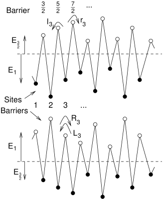
Figure 1: (Top) Illustration of an ‘energy landscape’, defined in terms of site energies $E_{i}$ and transition state energies $E_{i+\frac{1}{2}}$. The rate for hopping from a site is related to the sum of the site energy (measured downwards as shown) and the adjacent transition state energy (measured upwards). (Bottom) On inversion of the potential, the transition state energies become energies of new sites with half-integer indices: transition rates between these sites are controlled by the energies $E_{i}$ which now have an interpretation as transition state energies. From Ref. JS-jstat.

In this section, we review some previous results [8], restricting our analysis to periodic chains. In this case we have, writing $W$ as $W^{(1)}$ to distinguish from the dual operator $W^{(1/2)}$ below,

$$W^{(1)}=\sum_{i=1}^{N}\big{(}|i+1\rangle-|i\rangle\big{)}\big{(}r_{i}\langle i|-\ell_{i+1}\langle i+1|\big{)}.$$ (3)

from which conservation of particles is apparent as $\sum_{i}\langle i|W^{(1)}=0$. This allows us to intepret $W^{(1)}$ as a master equation for stochastic motion of a single particle.

This hopping model is dual to a second model which is of the same form, but with hopping on sites with half-integer indices. That is, one has densities $n_{\frac{1}{2}}(t),n_{\frac{3}{2}}(t),\dots$, from which we construct a state $|\tilde{n}(t)\rangle=\sum_{i}n_{i-\frac{1}{2}}(t)|i-{\textstyle{\frac{1}{2}}}\rangle$ whose evolution is given by a master operator

$$W^{(1/2)}=\sum_{i=1}^{N}\left(|i+{\textstyle{\frac{1}{2}}}\rangle-|i-{\textstyle{\frac{1}{2}}}\rangle\right)\left(R_{i}\langle i-{\textstyle{\frac{1}{2}}}|-L_{i}\langle i+{\textstyle{\frac{1}{2}}}|\right).$$ (4)

Since the particles reside on half-integer sites, we associate integer indices with barriers between the sites. Thus, $L_{i}$ and $R_{i}$ are rates for motion to left and right across the $i$th barrier. Then, $W^{(1)}$ is dual to $W^{(1/2)}$ if we take

$$L_{i}=r_{i},\qquad R_{i}=\ell_{i}$$ (5)

whose physical interpretation as an inversion of the energy landscape will be discussed below (see also Fig. 1).

To reveal the duality between the models, we write

$$D = \sum_{i=1}^{N}\big{(}|i\rangle-|i+1\rangle\big{)}\langle i+{\textstyle{\frac{1}{2}}}|,$$

$$J = \sum_{i=1}^{N}|i+{\textstyle{\frac{1}{2}}}\rangle\big{(}r_{i}\langle i|-\ell_{i+1}\langle i+1|\big{)},$$ (6)

so that

$$W^{(1)}=-DJ,\qquad W^{(1/2)}=-(JD)^{\dagger}.$$ (7)

This factorisation means that $W^{(1)}$ and $W^{(1/2)}$ have the same eigenspectra. For example, if $\langle\psi|$ is a left eigenvector of $W^{(1)}$ with eigenvalue $\lambda\neq 0$ then $D^{\dagger}|\psi\rangle$ is a right eigenvector of $W^{(1/2)}$ with the same eigenvalue. To express this duality in a more standard form, we could write

$$W^{(1)}D=-DJD=D(W^{(1/2)})^{\dagger}.$$ (8)

Despite the simple form of (5), we emphasise that this duality relates distinct pairs of hopping models. To illustrate this, we parameterise the rates in a region of the chain as

$$\ell_{i}=\mathrm{e}^{-E_{i}-E_{i-\frac{1}{2}}},\qquad r_{i}=\mathrm{e}^{-E_{i}-E_{i+\frac{1}{2}}}$$ (9)

where we interpret the $E_{i}$ and $E_{i+\frac{1}{2}}$ as site and transition state energies. The duality condition (5) can then be interpreted as a swap of transition state and site energies, or equivalently as an inversion of the energy landscape, as in Fig. 1. Our sign convention is that the $E_{i}$ are measured downwards from an arbitrary baseline, so that site and transition energies are dual to each other. We note that a parameterisation of the rates in the form (9) is always possible on any subsection of the chain, but applying it to the whole set of rates requires additionally a global constraint of detailed balance: $\prod_{i}r_{i}=\prod_{i}\ell_{i}$.

In addition, one may relate the propagators within the two models. Interpreting the equations of motion (1) as a master equation for a single particle we identify the propagator $G^{(1)}_{ij}(t)=\langle i|\mathrm{e}^{W^{(1)}t}|j\rangle$ as the probability that the particle is on site $i$ given that it was on site $j$ a time $t$ earlier. In the description in terms of non-interacting particles, the steady state two-point connected correlation function is simply

$$\langle n_{i}(t)n_{j}(0)\rangle_{\mathrm{ss}}-\langle n_{i}\rangle_{\mathrm{ss}}\langle n_{j}\rangle_{\mathrm{ss}}=G_{ij}(t)\langle n_{j}\rangle_{\mathrm{ss}}$$ (10)

where we use the label ‘ss’ to indicate a steady state average. Starting from (8), we consider the matrix elements $\langle i|\mathrm{e}^{W^{(1)}t}D|j-\frac{1}{2}\rangle=\langle i|D\mathrm{e}^{(W^{(1/2)})^{\dagger}t}|j-\frac{1}{2}\rangle$, arriving at

$$G^{(1)}_{ij}(t)-G^{(1)}_{i,j-1}(t)=G^{(1/2)}_{j-\frac{1}{2},i-\frac{1}{2}}-G^{(1/2)}_{j-\frac{1}{2},i+\frac{1}{2}}$$ (11)

where $G^{(1/2)}_{i+\frac{1}{2},j+\frac{1}{2}}(t)=\langle i+{\textstyle{\frac{1}{2}}}|\mathrm{e}^{W^{(1/2)}t}|j+{\textstyle{\frac{1}{2}}}\rangle$ is the propagator in the dual model. We emphasise that such results have application beyond single-particle models: for example, the same relation applies to models of diffusing and annihilating defects in random potentials [6] (with some restrictions on boundary conditions).

Importantly, Equ. (11) allows the propagator in the dual model to be calculated from that of the original model, without any knowledge of the disorder. If one then chooses the $r_{i}$ and $\ell_{i}$ from (different) distributions that are independent under translation in space then one may prove that the disorder-averaged propagators satisfy

$$\overline{G}^{(1)}_{ij}(t)=\overline{G}^{(1/2)}_{ij}(t)$$ (12)

with both sides depending only on the difference $i-j$.

Returning to models with detailed balance, $\prod_{i}\ell_{i}=\prod_{i}r_{i}$, we now define an operator $\hat{E}^{(1)}$ such that $\hat{E}^{(1)}|i\rangle=E_{i}|i\rangle$ and similarly $\hat{E}^{(1/2)}$ such that $\hat{E}^{(1/2)}|i+{\textstyle{\frac{1}{2}}}\rangle=E_{i+\frac{1}{2}}|i+{\textstyle{\frac{1}{2}}}\rangle$. Then, taking

$$S=-D\mathrm{e}^{-\hat{E}^{(1/2)}} = \sum_{i=1}^{N}\left(|i+1\rangle-|i\rangle\right)\langle i+{\textstyle{\frac{1}{2}}}|\mathrm{e}^{-E_{i+\frac{1}{2}}}$$ (13)

$$\overline{S}=D^{\dagger}\mathrm{e}^{-\hat{E}^{(1)}} = \sum_{i=1}^{N}\left(|i+{\textstyle{\frac{1}{2}}}\rangle-|i-{\textstyle{\frac{1}{2}}}\rangle\right)\langle i|\mathrm{e}^{-E_{i}}$$ (14)

we arrive at a more symmetric factorisation of the master operators [8]:

$$W^{(1)}=S\overline{S},\qquad W^{(1/2)}=\overline{S}S.$$ (15)

We previously considered consequences of this symmetric factorisation [8], and defined a renormalisation scheme that acts symmetrically on $S$ and $\overline{S}$. For the purposes of this paper, the key point is that detailed balance ensures that $W^{(1/2)}\mathrm{e}^{-\hat{E}^{(1/2)}}=\mathrm{e}^{-\hat{E}^{(1/2)}}(W^{(1/2)})^{\dagger}$ (and similarly for $W^{(1)}$). This additional symmetry of the master operators allows the symmetric factorisation of (15), which also implies additional ‘duality’ relations $W^{(1)}S=SW^{(1/2)}$ and $\overline{S}W^{(1)}=W^{(1/2)}\overline{S}$. This structure appears in supersymmetric field theories [8, 11, 12]. In supersymmetric models the two symmetry relations are linked to time-translation invariance and time-reversal invariance [12] (via detailed balance and the fluctuation-dissipation theorem.)

3 Bulk-driven pure trap and barrier models

We now consider disordered systems with uniform driving forces applied throughout the system. This clearly breaks detailed balance and time-reversal symmetry. It is therefore somewhat surprising that we can identify a restricted set of such models for which a factorisation similar to (15) is possible. We will discuss how this factorisation reflects symmetries of the models under a change in the direction of the bias, at fixed disorder.

In this section, we restrict the form of the disorder to ‘pure trap’ and ‘pure barrier’ models. The former are obtained by setting $E_{i+\frac{1}{2}}=0$ for all $i$, but choosing the $E_{i}$ freely. Then, $W^{(1)}$ describes a pure trap model with $r_{i}=\ell_{i}=\mathrm{e}^{-E_{i}}$: site $i$ represents a trap from which particles hop to left and right with equal probability, but the overall rate depends on the trap depth $E_{i}$. We add a bias to this model by taking

$$r_{i}=x\mathrm{e}^{-E_{i}},\qquad\ell_{i}=y\mathrm{e}^{-E_{i}}.$$ (16)

We take $x+y=2$ for convenience since this factor simply rescales time, and we assume $x>1$ for concreteness. Pure barrier models are dual to pure trap models, so their sites have half-integer indices and their master operators are of the form $W^{(1/2)}$. In the absence of a bias, all sites have the same energy $E_{i}=0$, but rates for hopping between sites depend on the barrier being crossed. In the presence of a bias, right- and left-going rates are multiplied by $x$ and $y$ respectively.

The master operator for the trap model is constructed as in (7):

$$W^{\mathrm{rT}}=W^{(1)}=-DJ_{xy}$$ (17)

where the label ‘rT’ indicates that we consider a trap model biased to the right, and we indicate explicitly that the current operator $J$ depends on $x$ and $y$ (as well as on the $E_{i}$). One can then construct a master operator, $W^{\mathrm{\ell B}}=-(J_{xy}D)^{\dagger}$ that is dual to $W^{\mathrm{rT}}$, in accordance with (7). It has barrier-crossing rates $R_{i}=\ell_{i}=y\mathrm{e}^{-E_{i}}$ and $L_{i}=r_{i}=x\mathrm{e}^{-E_{i}}$ and is therefore biased to the left, justifying our notation $W^{\mathrm{\ell B}}$.

As noted above, these biased models do not respect detailed balance, so they may not be factorised as in (15). However, let $W^{\mathrm{\ell T}}$ be the master operator for a trap model with a bias to the left (that is, $W^{\mathrm{\ell T}}=-DJ_{yx}$). It may then be verified that

$$W^{\mathrm{\ell T}}=S^{\prime}_{yx}\overline{S},\qquad W^{\mathrm{\ell B}}=\overline{S}S^{\prime}_{yx}$$ (18)

where $\overline{S}$ was defined above, and

$$S^{\prime}_{yx} = \sum_{i=1}^{N}\left(y|i+1\rangle-x|i\rangle\right)\langle i+{\textstyle{\frac{1}{2}}}|$$ (19)

Thus, $W^{\mathrm{\ell B}}$ has two alternative factorisations, as $-(J_{xy}D)^{\dagger}$ from (7) and as $\overline{S}S^{\prime}_{yx}$. These relations show that it is dual both to $W^{\mathrm{rT}}$ and $W^{\mathrm{\ell T}}$, and all three operators share the same eigenspectrum. By eliminating $W^{\mathrm{\ell B}}$, one can then also write a simple duality between trap models with opposite biases,

$$W^{\mathrm{\ell T}}\mathrm{e}^{\hat{E}^{(1)}}=\mathrm{e}^{\hat{E}^{(1)}}(W^{\mathrm{rT}})^{\dagger}$$ (20)

This reflects a physical relation between time-reversed trajectories: a trajectory $\pi(t)$ in the right-biased trap model and the time-reversed trajectory $\bar{\pi}(t)$ in the left-biased model have the same probabilities in the steady state. Note here that both models have the same steady state densities as an unbiased trap model, $\langle n_{i}\rangle_{\mathrm{ss}}\propto\mathrm{e}^{E_{i}}$.

In an analogous manner we can eliminate $W^{\mathrm{\ell T}}$ from the duality relations that link it to $W^{\mathrm{rB}}$ and $W^{\mathrm{\ell B}}$ to get a duality relation between left- and right-biased barrier models:

$$W^{\mathrm{\ell B}}\overline{S}D=\overline{S}D(W^{\mathrm{rB}})^{\dagger}$$ (21)

where $\overline{S}D=D^{\dagger}\mathrm{e}^{-\hat{E}^{(1)}}D$. This equation also expresses a relation between propagation in the models, under inversion both of the bias and of the direction of time. However, we did not find any simple physical interpretaton of this relation.

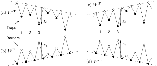
Figure 2: Illustration of (local) energy landscape for biased trap and barrier models, following Fig. 1. A landscape inversion as in Fig. 1 relates (a), a trap model biased to the right, to (b), a barrier model biased to the left. However, Equ. (20) means that (a) is also dual to (c), a trap model biased to the left. Finally, inverting the landscape (c) leads to (d), a barrier model biased to the right. Thus all four landscapes represent models with the same spectrum, as described in the text. We emphasise that the pairs (a,c) and (b,d) are related by an inversion of the bias, but with the disordered rates $E_{i}$ remaining invariant. The energy $E_{3}$ is identified for all four landscapes.

To understand the relationships between the four biased trap and barrier models, it is helpful to think in terms of tilted energy landscapes as shown in Fig. 2. Of course the bulk bias on an entire periodic chain cannot be represented in this way, but if we restrict attention to propagation over finite times $t$ and therefore finite regions of the chain, this is not an issue. For example, to parameterise the rates (16) of $W^{\mathrm{rT}}$ in terms of site and barrier energies as in (9), one may define $E_{j}^{\prime}=E_{j}+jF$ and $E_{j+\frac{1}{2}}^{\prime}=-(j+\frac{1}{2})F-\delta$ where $F=\ln(x/y)$ is the driving force (in units where the temperature and lattice spacing are unity) and $\delta=\frac{1}{2}\ln(x/y)$ is an offset to the transition state energies that simply acts to rescale the time in accordance with $x+y=2$. The situation is illustrated in Fig. 2(a). The factorization $W^{\mathrm{rT}}=-DJ_{xy}$ leads to the dual model $W^{\mathrm{\ell B}}=-(J_{xy}D)^{\dagger}$, a pure barrier model biased to the left as shown in Fig. 2(b). This model can alternatively be factorized as $\overline{S}S^{\prime}_{yx}$, which has as its dual $W^{\mathrm{\ell T}}=S^{\prime}_{yx}\overline{S}$, a trap model biased to the left (Fig. 2(c)).

These various symmetries also result in relations between propagators in the various models. If the propagator for one model (say the right-biased trap model) is known then those of its three dual models may be constructed. For example, (11) reads in the notation of this section

$$G^{\mathrm{rT}}_{ij}(t)-G^{\mathrm{rT}}_{i,j-1}(t)=G^{\mathrm{\ell B}}_{j-\frac{1}{2},i-\frac{1}{2}}(t)-G^{\mathrm{\ell B}}_{j-\frac{1}{2},i+\frac{1}{2}}(t)$$ (22)

independently of both bias and disorder; the labels on the propagators are the same as those on the associated operators $W$. However, noting that $W^{\mathrm{rT}}S^{\prime}_{xy}=S^{\prime}_{xy}W^{\mathrm{rB}}$ one may derive by a similar method

$$xG^{\mathrm{rT}}_{i,j+1}(t)-yG^{\mathrm{rT}}_{i,j}(t)=xG^{\mathrm{rB}}_{i-\frac{1}{2},j+\frac{1}{2}}(t)-yG^{\mathrm{rB}}_{i+\frac{1}{2},j+\frac{1}{2}}(t).$$ (23)

which is again independent of disorder but now depends on the bias. One may also use $\overline{S}W^{\mathrm{rT}}=W^{\mathrm{rB}}\overline{S}$ to arrive at a relation that depends on disorder but not on the bias. However, this last relation reduces to (22) if one notes simply that

$$G^{\mathrm{\ell T}}_{ij}(t)\mathrm{e}^{E_{j}}=G^{\mathrm{rT}}_{ji}(t)\mathrm{e}^{E_{i}}$$ (24)

which follows from (20). The latter relation between propagation in left- and right-biased trap models can also be written in a disorder-independent manner: for finite $t$ and hence $i-j$, the propagators obey detailed balance with respect to the effective energy landscape defined above, i.e. $G^{\mathrm{rT}}_{ji}\mathrm{e}^{E^{\prime}_{i}}=G^{\mathrm{rT}}_{ij}\mathrm{e}^{E^{\prime}_{j}}$. This transforms our last relation into

$$G^{\mathrm{\ell T}}_{ij}(t)=\left(\frac{y}{x}\right)^{i-j}G^{\mathrm{rT}}_{ij}(t)$$ (25)

which holds independently of the disorder as anticipated.

Finally, using (12) and taking the disorder average of (23), it may readily be shown that the disorder-averaged diffusion fronts in the various models are related as

$$\overline{G}^{\mathrm{rT}}_{i-j}(t)=\overline{G}^{\mathrm{rB}}_{i-j}(t)=\overline{G}^{\mathrm{\ell T}}_{j-i}(t)=\overline{G}^{\mathrm{\ell B}}_{j-i}(t)$$ (26)

Thus, in this section and the preceding one, we have shown how symmetries under time-reversal (detailed balance) or bias-inversion may be combined with the general relation (7), leading to symmetric factorisations such as (15) and (18). These relations allow the propagators of the models to be related to one another. They also reveal an intuitively reasonable link between left- and right-biased trap models, and a somewhat more surprising relation between left- and right-biased barrier models.

4 Boundary-driven case

We now turn to the boundary-driven hopping models described in Sec. 1. That is, the equations of motion are given by (1) for $i=1\dots N$ but we introduce two new time-independent reservoir densities, $n_{0}$ and $n_{N+1}$. The model depends on the rates $r_{0},\ell_{1},\dots,r_{N},\ell_{N+1}$ which may always be parameterised in terms of site and transition state energies as in (9). The dependence on the reservoir densities appears only through the combination $n_{0}r_{0}$ and $n_{N+1}\ell_{N+1}$, or equivalently, through $n_{0}\mathrm{e}^{-E_{0}}$ and $n_{N+1}\mathrm{e}^{-E_{N+1}}$. Since the particles are non-interacting, if we increase both $n_{0}$ and $n_{N+1}$ by a multiplicative factor this simply increases the total particle number by the same factor. Further, if the two reservoirs are at different chemical potentials, $n_{0}\mathrm{e}^{-E_{0}}-n_{N+1}\mathrm{e}^{-E_{N+1}}\neq 0$, there is a current proportional to this difference.

Writing $|n(t)\rangle=\sum_{i=0}^{N+1}n_{i}(t)|i\rangle$ as above (but now with reservoir sites included), the equation of motion takes the form $\frac{\partial}{\partial t}|P(t)\rangle=W^{\mathrm{d}}|P(t)\rangle$ where $W^{\mathrm{d}}$ is of the form given in (2). Since the sum in (2) runs only from $1$ to $N$, we have $\langle 0|W^{\mathrm{d}}=\langle N+1|W^{\mathrm{d}}=0$, consistent with time-independent reservoir densities. It may be verified that the total density in the model is no longer conserved, so that $W^{\mathrm{d}}$ is not a stochastic operator: $\sum_{i}\langle i|W^{\mathrm{d}}\neq 0$.

4.1 Duality relations

Recently, Tailleur, Kurchan and Lecomte [2, 3] considered boundary-driven models of interacting particles, and showed that they are dual to ‘equilibrium’ models that respect detailed balance. They further showed that this duality can be demonstrated for disordered non-interacting systems, in a many-body representation. Here, we use the methods of the previous sections to analyse the non-interacting case. Since we use a basis of one-particle densities instead of a many-body basis, our analysis is simpler.

We begin by factorising $W^{\mathrm{d}}$ as

$$W^{\mathrm{d}}=\Lambda S^{\mathrm{d}}\overline{S}^{\mathrm{d}}$$ (27)

with

$$S^{\mathrm{d}} = \sum_{i=0}^{N}(|i+1\rangle-|i\rangle)\langle i+{\textstyle{\frac{1}{2}}}|\mathrm{e}^{-E_{i+\frac{1}{2}}},$$ (28)

$$\overline{S}^{\mathrm{d}} = \sum_{i=0}^{N+1}|i-{\textstyle{\frac{1}{2}}}\rangle(\langle i-1|\mathrm{e}^{-E_{i-1}}-\langle i|\mathrm{e}^{-E_{i}}),$$ (29)

$$\Lambda = \sum_{i=1}^{N}|i\rangle\langle i|=1-|0\rangle\langle 0|-|N+1\rangle\langle N+1|.$$ (30)

In $\overline{S}^{\mathrm{d}}$, we identify site $-1$ with site $N+1$: we imagine a periodic chain with the reservoirs sites being adjacent, but we forbid direct hopping between the reservoirs by formally setting $\mathrm{e}^{-E_{-\frac{1}{2}}}=0$. This makes the duality relations simpler since there are then equal numbers of sites $i$ and transition states $i+\frac{1}{2}$. See Fig. 3.

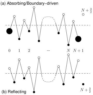
Figure 3: Illustration of energy landscape for boundary-driven models and models with reflecting and absorbing boundaries. We show only regions near the ends of the chain. (a) The boundary-driven and absorbing models have the same disorder: the large circles on sites $0$ and $N+1$ represent reservoirs for the driven case (operator $W^{\mathrm{d}}$) and absorbing sites for the absorbing boundaries (operators $W^{\mathrm{a}}$). There is an extra transition state on site $N+\frac{3}{2}$ to facilitate comparison of dual operators. (b) The model with reflecting boundaries (operator $W^{\mathrm{r}}$). The landscape is obtained by inverting that for the driven/absorbing systems, following the procedure of Fig. 1. There is an isolated site $N+\frac{3}{2}$, with no hopping in or out. This ensures that all operators act in spaces of dimension $N+2$.

Then, we define two new operators

$$W^{\mathrm{r}}=\overline{S}^{\mathrm{d}}\Lambda S^{\mathrm{d}},\qquad W^{\mathrm{a}}=S^{\mathrm{d}}\overline{S}^{\mathrm{d}}\Lambda$$ (31)

These operators describe hopping for conserved particles, with energy landscapes illustrated in Fig. 3. They all have equal eigenspectra: if $|\psi\rangle$ is a right eigenvector of $W^{\mathrm{d}}$ with eigenvalue $\lambda\neq 0$ then $\overline{S}^{\mathrm{d}}|\psi\rangle$ is a right eigenvector of $W^{\mathrm{r}}$ and $S^{\mathrm{d}}\overline{S}^{\mathrm{d}}|\psi\rangle$ is a right eigenvector of $W^{\mathrm{a}}$, all with the same eigenvector. These duality relations lead to the same conclusions as the many-body analysis of Ref. TKL-08 (for the non-interacting disordered case). Indeed, the many-body duality transformation considered there can be written compactly in terms of the matrix elements of $S^{\mathrm{d}}$ and $\overline{S}^{\mathrm{d}}$ [13]. Whether any similar transformation may be exploited in the systems of interacting particles considered in Refs. TKL-07,TKL-08 remains a question for future work.

4.2 Consequences of the duality symmetry

The duality symmetry allows relations between propagators in the models to be determined. In particular, for the steady state in the boundary-driven model, we have $\langle n_{i}(t)n_{j}(0)\rangle_{\mathrm{ss}}-\langle n_{i}\rangle_{\mathrm{ss}}\langle n_{j}\rangle_{\mathrm{ss}}=G^{\mathrm{d}}_{ij}(t)\langle n_{j}\rangle_{\mathrm{ss}}$ with $G^{\mathrm{d}}_{ij}(t)=\langle i|\mathrm{e}^{W^{\mathrm{d}}t}|j\rangle$. From the relation $\Lambda W^{\mathrm{a}}=W^{\mathrm{d}}\Lambda$, it follows that for $1\leq i,j\leq N$,

$$G^{\mathrm{d}}_{ij}(t)=G^{\mathrm{a}}_{ij}(t)$$ (32)

where $G^{\mathrm{a}}_{ij}(t)=\langle i|\mathrm{e}^{W^{\mathrm{a}}t}|j\rangle$ is the propagator for the model with absorbing states on sites $0$ and $N+1$. That is, steady state correlations in the boundary-driven steady state of the model $W^{\mathrm{d}}$ are equal to propagation probabilities between sites of a model with absorbing boundaries. Similar results for interacting models can also be derived [4]. Physically, one notes that once a particle visits a reservoir, all correlations associated with it are lost, so the non-trivial correlations in the boundary-driven and absorbing models are the same.

Further, the duality between models with reflecting and absorbing boundaries can be obtained by a factorisation, either as (7) or as (15). In the notation of this section, (11) reads:

$$G^{\mathrm{r}}_{i-\frac{1}{2},j-\frac{1}{2}}(t)-G^{\mathrm{r}}_{i-\frac{1}{2},j+\frac{1}{2}}(t) = G^{\mathrm{a}}_{ji}(t)-G^{\mathrm{a}}_{j,i-1}(t)$$ (33)

$$= G^{\mathrm{d}}_{ji}(t)-G^{\mathrm{d}}_{j,i-1}(t)$$

where we used (32) in the second equality and assumed $1\leq i,j\leq N$. Remarkably, this allows the two-point correlations of boundary-driven models to be constructed from the equilibrium correlations of a dual model ($W^{\mathrm{r}}$) with an inverted energy landscape but no net current.

5 Conclusion

We have discussed duality symmetries of non-interacting hopping models that are revealed by factorising their equations of motion. These factorisations indicate symmetries of the models. For example, if particles are conserved, master operators may be written as $W^{(1)}=-DJ$, allowing a dual model $W^{(1/2)}=-D^{\dagger}J^{\dagger}$ to be constructed as in (7). If the models have additional symmetry, these may be revealed through alternative factorisations such as $W^{(1)}=S\overline{S}$ for models obeying detailed balance, or $W^{\mathrm{rT}}=S^{\prime}_{xy}\overline{S}$ for driven trap models, leading to new dual models $W^{(1/2)}=\overline{S}S$ or $W^{\mathrm{rB}}=\overline{S}S^{\prime}_{xy}$. These factorisations and duality relations allow relationships between propagators within the various models to be derived.

For boundary-driven models without conserved currents, a factorisation of the master operator exists which reveals its duality with a model where particles are conserved and boundary conditions are reflecting, which we intepret as an ‘equilibrium’ model. This then also allows a further relation to be derived between the boundary-driven model and one with absorbing boundaries.

Several of these relations are known in models of interacting particles [2, 3, 5, 4, 6], although derivations in such models require considerably more detailed calculations. Whether the methods presented here can be used to interpret and generalise such relations remains a topic for future study.

References

- [1] For a review, see, for example, B. Derrida, J. Stat. Mech (2007) P07023.
- [2] J. Tailleur, J. Kurchan and V. Lecomte, Phys. Rev. Lett. 99 (2007), 150602.
- [3] J. Tailleur, J. Kurchan and V. Lecomte, J. Phys. A 41 (2008), 505001.
- [4] C. Giardina, J. Kurchan, F. Redig and K. Vafayi, J. Stat. Phys. 135 (2009), 25.
- [5] A. Imparato, V. Lecomte and F. van Wijland, Phys. Rev. E 80 (2009), 011131.
- [6] G. M. Schütz, Z. Phys. B 104 (1997), 583; G. M. Schütz and K. Mussawisade, Phys. Rev. E 57 (1998), 2564.
- [7] R. L. Jack and P. Sollich, J. Phys. A 41 (2008), 324001.
- [8] R. L. Jack and P. Sollich, J. Stat. Mech (2009), P11011.
- [9] E. Bertin, J.-P. Bouchaud and F. Lequeux, Phys. Rev. Lett. 95 (2005), 015702; R. L. Jack, P. Sollich and P. Mayer, Phys. Rev. E 78 (2008), 061107.
- [10] For reviews, see S. Alexander et al., Rev. Mod. Phys. 53 (1981), 175; J.-P. Bouchaud and A. Georges, Phys Rep 195 (1990), 127; R. Metzler and J. Klafter, Phys. Rep. 339 (2000), 1.
- [11] S. Tanase-Nicola and J. Kurchan, Phys. Rev. Lett. 91 (2003), 188302; S. Tanase-Nicola and J. Kurchan, J. Stat. Phys. 116 (2004), 1201.
- [12] J. Zinn-Justin, Quantum Field Theory and Critical Phenomena, chapter 17 (Oxford University Press, Oxford, 2002)
- [13] R. L. Jack and P. Sollich, unpublished.