Two-photon and one photon-one vector meson decay widths of the $f_{0}(1370)$, $f_{2}(1270)$, $f_{0}(1710)$, $f^{\prime}_{2}(1525)$, and $K^{*}_{2}(1430)$

Abstract

We calculate the radiative decay widths, two-photon ($\gamma\gamma$) and one photon-one vector meson ($V\gamma$), of the dynamically generated resonances from vector meson-vector meson interaction in a unitary approach based on the hidden-gauge Lagrangians. In the present paper we consider the following dynamically generated resonances: $f_{0}(1370)$, $f_{0}(1710)$, $f_{2}(1270)$, $f_{2}^{\prime}(1525)$, $K^{*}_{2}(1430)$, two strangeness=0 and isospin=1 states, and two strangeness=1 and isospin=1/2 states. For the $f_{0}(1370)$ and $f_{2}(1270)$ we reproduce the previous results for the two-photon decay widths and further calculate their one photon-one vector decay widths. For the $f_{0}(1710)$ and $f_{2}^{\prime}(1525)$ the calculated two-photon decay widths are found to be consistent with data. The $\rho^{0}\gamma$, $\omega\gamma$ and $\phi\gamma$ decay widths of the $f_{0}(1370)$, $f_{2}(1270)$, $f_{0}(1710)$, $f^{\prime}_{2}(1525)$ are compared with the results predicted by other approaches. The $K^{*+}\gamma$ and $K^{*0}\gamma$ decay rates of the $K^{*}_{2}(1430)$ are also calculated and compared with the results obtained in the framework of the covariant oscillator quark model. The results for the two states with strangeness=0, isospin=1 and two states with strangeness=1, isospin=1/2 are predictions that need to be tested by future experiments.

I Introduction

One of the central topics in studies of low-energy strong interaction is to understand how quarks and gluons combine into hadronic objects that we observe experimentally, in other words, to understand low-energy meson and baryon spectroscopy. Unfortunately, the non-perturbative nature of QCD at low-energies has made a complete solution of this problem from first principles almost impossible (admittedly, lattice QCD has made remarkable progress in recent years, and may provide a solution in the future). Furthermore, most of the observed hadronic states are not asymptotic states, and as such, they appear only in invariant mass distributions, phase shifts, etc. This latter feature then implies that in many cases one can not ignore final state interaction among their decay products.

A prominent example is the existence and nature of the $f_{0}(600)$. For a comprehensive discussion and references, see the mini-review “Note on scalar mesons” of Ref. Amsler:2008zzb . Although its existence has long been hypothesized, it took quite a long time until different experiments have finally pinned it down unanimously. Its nature is even more troubling, i.e., whether it is a genuine $q\bar{q}$ state, $qq\bar{q}\bar{q}$ state, or molecular state. In this context, the unitarization technique in combination with the chiral Lagrangians, the so-called unitary chiral theories, have provided a self-consistent picture where the $f_{0}(600)$ may be due to the $\pi\pi$ final state interactions Oller:1997ti ; Kaiser:1998fi ; Markushin:2000a ; Dobado:1997a ; ramonet . The same approach has been used to study various other hadronic systems, e.g., the kaon-nucleon system Kaiser:1995eg ; Oset:1998a ; ollerulf ; Recio:2004a ; Jido:2003a ; Recio:2006a ; Hyodo:2003a ; Borasoy:2005a ; Oller:2005a ; Borasoy:2006a , heavy-light systems Kolomeitsev:2003ac and three body systems MartinezTorres:2007sr .

The unitary chiral approach, however, can only be employed to study interactions among the Goldstone-bosons themselves and those between them and other hadrons, because chiral symmetry only defines the interactions involving the Goldstone-bosons. One may think about applying the same unitarization technique to study other systems by employing phenomenological Lagrangians. In Refs. Molina:2008jw ; Gonzalez:2008pv ; Sarkar:2009kx ; Molina:2009eb ; Oset:2009vf ; Geng:2008gx , by combining the phenomenologically successful hidden-gauge Lagrangians with the above-mentioned unitarization technique, the interactions of vectors mesons among themselves and with octet- and decuplet-baryons have been studied. In the framework of this approach many interesting results have been obtained, which all compare rather favorably with existing data. The dynamically generated resonances should contain sizable meson-meson or meson-baryon components in their wave-functions, thus qualifying as “molecular states.”

Whether such a picture is correct or partially correct has ultimately to be judged either by data or by studies based on first principles (e.g., lattice QCD calculations). From the first perspective, one should test as extensively as possible whether the proposed picture is consistent with (all) existing data, make predictions, and propose experiments where such predictions can be tested. These would provide further support to, or reject, the proposed nature of these states as being dynamically generated.

In the case of the vector meson–vector meson molecular states obtained in Refs. Molina:2008jw ; Geng:2008gx , several such tests have been passed: In Refs. Geng:2008gx ; Geng:2009gb it has been shown that the branching ratios into pseudoscalar-pseudoscalar and vector-vector final states of the $f_{0}(1370)$, $f_{0}(1710)$, $f_{2}(1270)$, $f_{2}^{\prime}(1525)$, and $K_{2}^{*}(1430)$ are all consistent with data. In Ref. Nagahiro:2008um , the two-photon decay widths of the $f_{0}(1370)$ and $f_{2}(1270)$ have been calculated and found to agree with data. Furthermore, in Ref. MartinezTorres:2009uk , the ratios of the $J/\psi$ decay rates into a vector meson ($\phi$, $\omega$, or $K^{*}$) and one of the tensor states [$f_{2}(1270)$, $f_{2}^{\prime}(1525)$, and $K^{*}_{2}(1430)$] have been calculated, and the agreement with data is found to be quite reasonable. Following the same approach, in Ref. Geng:2009iw it is shown that the ratio of the $J/\psi$ decay rates into $\gamma f_{2}(1270)$ and $\gamma f^{\prime}_{2}(1525)$ also agrees with data.

The radiative decay of a mesonic state has long been argued to be crucial in determinations of the nature of the state Pennington:2008qa . For instance, the non-observation of the $f_{0}(1500)$ decaying into two photons has been used to support its dominant glue nature Amsler:2002ey . In Ref. Nagahiro:2008um , the two-photon decay widths of the $f_{0}(1370)$ and $f_{2}(1270)$ have been calculated and found to agree with data which therefore provides further support to the proposed $\rho\rho$ molecular nature of these states Molina:2008jw . In the present paper, we extend our previous work to the $f_{0}(1710)$, $f_{2}^{\prime}(1525)$, $K^{*}_{2}(1430)$, and four other states dynamically generated from vector meson – vector meson interaction Geng:2008gx . By taking into account all the SU(3) allowed coupled channels, we also recalculate the two-photon decay widths of the $f_{0}(1370)$ and $f_{2}(1270)$, which confirms the earlier results of Ref. Nagahiro:2008um and provides a natural estimate of inherent theoretical uncertainties. We will also calculate the one photon-one vector meson decay widths of these resonances. As we will show below, in contrast to the results obtained in other theoretical models, our results show some distinct patterns, which should allow one to distinguish between different models once data are available.

This paper is organized as follows: In Section 2, we explain in detail how to calculate the two-photon and one photon-one vector meson decay widths of the dynamically generated states. In Section 3, we compare the results with those obtained in other approaches and available data, followed by a brief summary in Section 4.

II Formalism

II.1 Dynamically generated resonances from the vector meson-vector meson interaction

In the following, we briefly outline the main ingredients of the unitary approach (details can be found in Refs. Molina:2008jw ; Geng:2008gx ). There are two basic building-blocks in this approach: transition amplitudes provided by the hidden-gauge Lagrangians Bando:1984ej and a unitarization procedure. We adopt the Bethe-Salpeter equation method $T=(1-VG)^{-1}V$ to unitarize the transition amplitudes $V$ for $s$-wave interactions, where $G$ is a diagonal matrix of the vector meson-vector meson one-loop function

$$i\int\frac{d^{4}q}{(2\pi)^{4}}\frac{1}{q^{2}-M_{1}^{2}}\frac{1}{q^{2}-M_{2}^{2}}$$ (1)

with $M_{1}$ and $M_{2}$ the masses of the two vector mesons.

In Refs. Molina:2008jw ; Geng:2008gx three mechanisms, as shown in Fig. 1, have been taken into account for the transition amplitudes $V$: the four-vector contact term, the t(u)-channel vector exchange amplitude, and the direct box amplitude with two intermediate pseudoscalar mesons. Other possible mechanisms, e.g. s-channel vector exchange, crossed box amplitudes and box amplitudes involving anomalous couplings, have been neglected, since their contribution was found to be quite small in the detailed study of $\rho\rho$ scattering in Ref. Molina:2008jw .

Figure 1: Transition amplitudes $V$ appearing in the coupled-channel Bethe-Salpeter equation.

Among the three mechanisms considered for $V$, the four-vector contact term and $t(u)$-channel vector exchange one are responsible for the formation of resonances or bound states provided that the interaction generated by them is strong enough. In this sense, the dynamically generated states can be thought of as “vector meson-vector meson molecules.” On the other hand, the consideration of the imaginary part of the direct box amplitude allows the generated states to decay into two pseudoscalars. It should be stressed that in the present approach these two mechanisms play quite different roles: the four-vector contact interaction and the $t(u)$-channel vector exchange term are responsible for generating the resonances or bound states, whereas the direct box amplitude mainly contributes to their decays. This particular feature has an important consequence for the calculation of the radiative decay widths of the dynamically generated states as shown below.

The one-loop function, Eq. (1), is divergent and has to be regularized. In Ref. Geng:2008gx , both dimensional regularization method and cutoff method have been used. The couplings of the dynamically generated states to their coupled channels are given in Tables I, II, and III of Ref. Geng:2008gx , which we need to calculate the radiative decay widths of these resonances as explained below. In Ref. Geng:2008gx , the couplings were obtained on the second Riemann sheet using the dimensional regularization method without including the box diagrams in the model. If, instead, the loop functions were regularized using the cutoff method, one had to calculate the couplings from the modulus of amplitude squared on the real axis as done in Ref. Nagahiro:2008um . These two approaches were found to yield consistent values for the couplings. One has also some freedom in the values of the subtraction constants due to data uncertainty and the coupled-channel nature of the problem. An analysis of the resulting uncertainties has been performed in Refs. MartinezTorres:2009uk ; Geng:2009iw . They, however, were found to translate into small uncertainties (at the order of a few percent) in the present calculation.

We take advantage here to clarify a question often raised in connection with the dynamically generated states. Since we all accept that quarks are present in the physical mesons, the obvious question is what happens to the ordinary $q\bar{q}$ states? The answer to this can be found in the works of Refs. tornqvist1 ; tornqvist2 ; beveren ; boglione . In those works, where the study of the scalar mesons is addressed, one starts with a seed of $q\bar{q}$ states representing scalar states around $1.4$ GeV. Yet, these states unavoidably couple to meson meson components. This is a necessity imposed by unitarity, since the meson meson decay channels certainly couple to the physical states. Invoking symmetries, like SU(3), other meson meson channels, even those closed for the decay, will also couple to those $q\bar{q}$ components. For instance the $f_{0}(980)$ resonance decays into $\pi\pi$, so this must be a necessary coupled channel. However, the underlying SU(3) symmetry of the strong interactions will impose also the coupling to the $K\bar{K}$ component. One rightly guesses that other channels with masses far away from that of the $f_{0}(980)$ will play a minor role and can be neglected (actually they can be accounted for, as we shall discuss below). Then one has a coupled channel problem with $q\bar{q}$, $\pi\pi$ and $K\bar{K}$. According to Refs. tornqvist1 ; tornqvist2 ; beveren ; boglione the solution of the coupled channel problem leads to the scalar states where the original $q\bar{q}$ states are represented by a component of the wave function of minor importance, since the meson meson cloud has taken over and represents the bulk of the wave function. In simple words we can give a picture for this situation. As is well known, when we give energy to a hadron to break it and eventually see the quark components, we do not see the quarks, we see mesons produced. This seems to be the case not only when we break the hadron but when we excite it, such that the creation of mesons becomes energetically more favorable that the excitation of the quarks. One can easily visualize this in the baryon spectrum: either the Roper or the N*(1535) resonances would require 500-600 MeV of quark excitation energy, if they correspond to genuine quark excitations. It is clear that the introduction of a pion on top of the nucleon is energetically more favorable, so one should investigate the pion nucleon dynamics (together with other SU(3) related coupled channels) to see if this dynamics is able to produce these states. Indeed, the N*(1535) appears as dynamically generated from the meson baryon interaction in coupled channels kaiser ; inoue .

One can then still rightfully ask where the quark states go. Are there within this picture states that are mostly of $q\bar{q}$ nature? The answer is yes in principle, but nothing can guarantee it. One might think that they should appear at higher energies given the large energy needed to excite quarks. However, this is not necessarily true as we shall comment at the end of this section. On the other hand, the meson meson channels of smaller energy will be open. This detail should not go unnoticed. Indeed, let us think of a single channel problem with an attractive potential. One can get many discrete bound states in principle. Let us add another channel with an attractive potential, which by itself also generates discrete bound states. When we allow some coupling among these two channels then the earlier initial states give rise to two orthogonal combinations of the two channels. One might expect the same thing when we put together meson and quark channels. Yet, the counting of states does not follow here because for higher energies the meson meson channel will be unbound and then we can have a continuum of states. We can of course find out resonances, but this is not guaranteed nor is there any rule on how many resonances should appear. It all depends on the dynamics. The problem is indeed very interesting, but as far as one restricts oneself to low-lying resonances the meson meson nature is prominent and the effective Lagrangians used to take care of their interaction lead naturally to some bound states, which are those we consider. As to whether there are other states of simpler quark nature, in our approach we cannot say anything since these components are not part of our coupled channels states. However, apart from the works mentioned earlier tornqvist1 ; tornqvist2 ; beveren there are works in this direction in Refs. vijande ; vijande2 , which also conclude that the states of lower energy are mostly of mesonic nature.

Continuing with these observations, in connection with the quark components one can say that even the small admixture of these quark components could change the mass and other properties of the resonances. This might be so to some extent, but the studies with chiral dynamics and only hadron components have an element in the formalism which allows one to take this into account in an effective way. This is the subtraction constant in the $G$ function when the dimensional regularization formula is used, or the cut off in the cut off method. The basic idea of having the hadronic components as main building blocks is that the spectra is obtained using a natural value for the cut off or the subtraction constant ollerulf . Fine tuning of these subtraction constant or cut off can take into account the contribution from additional channels not explicitly considered in the approach, like the quark states hyodo ; bugg . In fact sometimes one needs a massive change of the cut off to reproduce the mass of a particle, which is a clear manifestation that the state under consideration is not of hadronic, but more of quark nature. This is the case for the $\rho$ meson, which does not come as an object made of $\pi\pi$. In the study of $\pi\pi$ scattering using the lowest-order chiral Lagrangians it would require a cut off of the order of several TeV, which is obviously far away from the natural scale of 1 GeV in effective theories of the low energy hadron spectra ramonet ; jose1 ; jose2 .

Actually the case of the $\rho$ is a good example of warning concerning the dynamical generation of resonances. If in the $\pi\pi$ interaction one takes the leading- and next-to-leading-order of the $s$-channel $\rho$-exchange amplitude and unitarizes it with the IAM (inverse amplitude method) or the Bethe Salpeter equation, one obtains the full amplitude (see section III of Ref. ramonet ). This is further elaborated in Ref. giacosa1 , which warns that this can happen in unitarization procedures, inducing one to think that one obtains a dynamically generated resonance, when in fact one is merely regenerating a preexisting resonance, which has been integrated out of the original Lagrangian and is not contained in the effective Lagrangian as a fundamental field. Although this warning should be kept in mind, one should also note that apart from regenerating a preexisting resonance, one can, and does in practice, generate other non-preexisting ones due to other terms in the potential, different from those directly associated to the $s$-channel exchange of the preexisting resonance, like contact terms and $t$- and $u$-channel exchange of those preexisting resonances. This is particularly clear in the case of the low-lying scalar mesons, which have different quantum numbers than the $\rho$. The latter, as mentioned above, would be “regenerated” in the unitarization scheme using the leading- and next-to-leading-order terms in the potential.

Nevertheless, in spite of all the arguments given in favor of the dynamically generated vector-vector states, the fact remains that the tensor states $f_{2}(1270)$, $f^{\prime}_{2}(1525)$, $a_{2}(1320)$, $K^{*}_{2}(1430)$ are well reproduced in the quark model, including many of their decay modes (see, e.g., Ref. Li:2000zb ; klempt ; crede ; isgur ; Barnes:1996ff ; Barnes:2002mu ; Anisovich:2002im ). This success in both models may reflect the fact that the constituent quarks in quark models are objects effectively dressed with meson clouds and the overlap between the molecular picture and the quark model picture could be bigger than expected in some cases gonzalez . Yet, even in this case, using one picture or the other could be more suited for other observables than those where the two models succeed. It is thus worth working with both models to make predictions. As we shall see in Section III, there are some observables where the predictions of the two models are indeed rather different.

II.2 Radiative decays, $\gamma\gamma$ and $V\gamma$, of the dynamically generated resonances

A detailed explanation of the two-photon decay mechanism has been given in Ref. Nagahiro:2008um . Here, we follow closely Ref. Nagahiro:2008um and extend it to the case of one photon-one vector meson decay.

The coupling of a photon to a dynamically generated resonance goes through couplings to its coupled-channel components in all possible ways such that gauge invariance is conserved (see, e.g, Refs. Nacher:1999ni ; Borasoy:2007ku for a relevant discussion within the kaon-nucleon system). A peculiar feature of the hidden-gauge Lagrangians is that photons do not couple directly to charged vector mesons but indirectly through their conversion to $\rho^{0}$, $\omega$, and $\phi$. This, together with the fact that the four-vector contact and the t(u)-channel exchange diagrams are responsible for the generation of the resonances or bound states, imply that the coupling of a photon to the resonance (or bound state) can be factorized into a strong part and an electromagnetic part Nagahiro:2008um : i.e., the resonance first decays into two vector mesons and then one or both of them convert into a photon. This is demonstrated schematically in Fig. 2 for the case of the two-photon decay. In the case of one photon-one vector meson decay, one simply replaces one of the final photons by one vector meson.

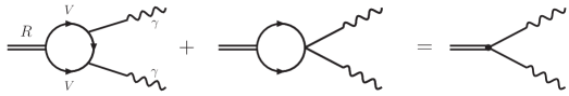
Figure 2: Two-photon decay of a dynamically generated resonance from vector meson-vector meson interaction.

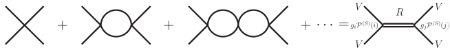
Figure 3: Pole representation of the vector-vector scattering amplitude and the definition of couplings of a dynamically generated resonance to its components.

Close to a pole position, the vector-vector scattering amplitude given in Fig. 3 can be parameterized as

$$T_{ij}^{(S)}=g_{i}\mathcal{P}^{(S)}(i)\frac{1}{s-M_{R}^{2}+iM_{R}\Gamma_{R}}g_{j}\mathcal{P}^{(S)}(j)$$ (2)

where $\mathcal{P}^{(S)}$ is the spin projection operator, which projects the initial (final) vector meson-vector meson pair $i$ ($j$) into spin $S$ with

$$\mathcal{P}^{(0)}=\frac{1}{\sqrt{3}}\epsilon_{i}(1)\epsilon_{i}(2),$$ (3)

$$\mathcal{P}^{(1)}=\frac{1}{2}\big{[}\epsilon_{i}(1)\epsilon_{j}(2)-\epsilon_{j}(1)\epsilon_{i}(2)\big{]},$$ (4)

$$\mathcal{P}^{(2)}=\frac{1}{2}\big{[}\epsilon_{i}(1)\epsilon_{j}(2)+\epsilon_{j}(1)\epsilon_{i}(2)\big{]}-\frac{1}{3}\epsilon_{m}(1)\epsilon_{m}(2)\delta_{ij},$$ (5)

where $\epsilon(1)$ [$\epsilon(2)$] is the polarization vector of particle 1 [2] and $i$, $j$, $m$ runs from 1 to 3 since in line with the approximation made in Refs. Molina:2008jw ; Geng:2008gx that $|\vec{p}|\,/M_{V}$ is small and hence $\epsilon_{0}=0$. The couplings $g_{i}$ ($g_{j}$) are obtained from the resonance pole position on the complex plane and are tabulated in Ref. Geng:2008gx . To evaluate the two-photon and one photon-one vector partial decay widths of the dynamically generated particles, one needs its coupling to the vector-vector components, i.e., $g_{i}\mathcal{P}^{(S)}_{i}$.

The amplitude of a neutral non-strange vector meson converting into a photon is given by

$$t_{V\gamma}=\mathcal{C}_{V\gamma}\frac{e}{g}M_{V}^{2}\epsilon^{\mu}(V)\epsilon_{\mu}(\gamma)\;\mbox{with}\;\mathcal{C}_{V\gamma}=\left\{\begin{array}[]{l}\frac{1}{\sqrt{2}}\;\mbox{for $\rho^{0}$}\\ \frac{1}{3\sqrt{2}}\;\mbox{for $\omega$}\\ -\frac{1}{3}\;\mbox{for $\phi$}\end{array}\right.,$$ (6)

with $g=\frac{m_{\rho}}{2f_{\pi}}$. Therefore, the whole two-photon and one photon-one vector decay amplitudes for a resonance $R$ of spin $S$ are

$$T^{(R)}(\gamma\gamma)\propto\sum\limits_{V_{1},V_{2}}g^{(R)}_{V_{1}V_{2}}{\cal P}^{(S)}_{V_{1}V_{2}}\left(\frac{1}{-M_{V_{1}}^{2}}\right)t_{V_{1}\gamma}\left(\frac{1}{-M_{V_{2}}^{2}}\right)t_{V_{2}\gamma}\times F_{1},$$ (7)

$$T^{(R)}(V_{1}\gamma)\propto\sum\limits_{V_{2}}g^{(R)}_{V_{1}V_{2}}{\cal P}^{(S)}_{V_{1}V_{2}}\left(\frac{1}{-M_{V_{2}}^{2}}\right)t_{V_{2}\gamma}\times F_{1},$$ (8)

where $F_{1}$ is a proper isospin coefficient which projects the vector-vector pair in isospin space to that in physical space and $g_{V_{1}V_{2}}^{(R)}$ denotes the coupling of resonance $R$ to channel $V_{1}V_{2}$. Recall that in Ref. Geng:2008gx we have used the following phase conventions: $K^{*-}=-|1/2,-1/2\rangle$ and $\rho^{+}=-|1,+1\rangle$, which implies that

$$|\rho\rho\rangle_{I=0} = -\frac{1}{\sqrt{3}}|\rho^{+}\rho^{-}+\rho^{-}\rho^{+}+\rho^{0}\rho^{0}\rangle,$$

$$|\rho K^{*}\rangle_{I=1/2,I_{3}=1/2} = -\sqrt{\frac{2}{3}}|\rho^{+}K^{*0}\rangle-\sqrt{\frac{1}{3}}|\rho^{0}K^{*+}\rangle,$$ (9)

$$|\rho K^{*}\rangle_{I=1/2,I_{3}=-1/2} = \sqrt{\frac{1}{3}}|\rho^{0}K^{*0}\rangle-\sqrt{\frac{2}{3}}|\rho^{-}K^{*+}\rangle.$$

From Eq. (II.2), one can easily read off the isospin projector $F_{1}$.

Summing over polarization of the intermediate vector mesons in Eqs. (7,8) and taking into account symmetry factors and proper normalization, one has the following amplitudes

$$T^{(R)}_{\gamma\gamma} = \frac{e^{2}}{g^{2}}\sum\limits_{V_{1},V_{2}=\rho^{0},\omega,\phi}g^{(R)}_{V_{1}V_{2}}\mathcal{P}^{(S)}_{\gamma\gamma}{\cal C}_{V_{1}\gamma}{\cal C}_{V_{2}\gamma}\times F_{1}\times F_{2}$$ (10)

$$T^{(R)}_{V_{1}\gamma} = \frac{e}{g}\sum\limits_{V_{2}=\rho^{0},\omega,\phi}g^{(R)}_{V_{1}V_{2}}\mathcal{P}^{(S)}_{V_{1}\gamma}{\cal C}_{V_{2}\gamma}\times F_{1}\times F_{3}$$ (11)

where $\mathcal{P}^{(S)}_{V\gamma}$ and $\mathcal{P}^{(S)}_{\gamma\gamma}$ are defined in Eqs. (3,4,5) with $V$ ($\gamma$) denoting the polarization vector of a vector-meson (photon); $F_{1}$ is the isospin factor, and $F_{2}$, $F_{3}$ account for both a symmetry factor and the unitary normalization used in Refs. Molina:2008jw ; Geng:2008gx

$$F_{2}=\Bigg{\{}\begin{array}[]{ll}\sqrt{2}&\text{ for a pair of identical particles, e.g. $\rho^{0}\rho^{0}$}\\ 2&\text{ for a pair of different particles, e.g. $\rho^{0}\omega$}\end{array},$$ (12)

$$F_{3}=\Bigg{\{}\begin{array}[]{ll}\sqrt{2}&\text{ for a pair of identical particles, e.g. $\rho^{0}\rho^{0}$}\\ 1&\text{ for a pair of different particles, e.g. $\rho^{0}\omega$}\end{array}.$$ (13)

The two-photon and one photon-one vector decay widths of a dynamically generated resonance $R$ of spin $S$ are then given by

$$\Gamma_{\gamma\gamma} = \frac{1}{2S+1}\frac{1}{16\pi M_{R}}\frac{1}{2}\times\sum\limits_{\mbox{polarization}}|T^{(R)}_{\gamma\gamma}|^{2},$$ (14)

$$\Gamma_{V\gamma} = \frac{1}{2S+1}\frac{1}{8\pi M_{R}}\frac{|p_{\gamma}|}{M_{R}}\times\sum\limits_{\mbox{polarization}}|T^{(R)}_{V\gamma}|^{2},$$ (15)

where $M_{R}$ is the resonance mass and $p_{\gamma}$ is the photon momentum in the rest frame of the resonance $R$. For the photon, we work in the Coulomb gauge ($\epsilon^{0}=0$ and $\vec{k}\cdot\vec{\epsilon}=0$), where the sum over the final polarizations are given by

$$\sum_{\mbox{polarization}}\epsilon_{i}(\gamma)\epsilon^{*}_{j}(\gamma)=\delta_{ij}-\frac{k_{i}k_{j}}{|\vec{k}|^{2}}$$ (16)

with $\vec{k}$ the three momentum of the photon. For vector mesons, one has $\epsilon_{0}=0$ [see discussion below Eq. (5)] and

$$\sum_{\mbox{polarization}}\epsilon_{i}(V)\epsilon^{*}_{j}(V)=\delta_{ij}.$$ (17)

With Eqs. (16,17), one can easily verify

$$\sum\limits_{\mbox{polarization}}{\cal P}^{(S)}_{\gamma\gamma}{\cal P}^{*(S)}_{\gamma\gamma}=\left\{\begin{array}[]{ll}\frac{2}{3}&S=0\\ 1&S=1\\ \frac{7}{3}&S=2\end{array}\right.,$$ (18)

$$\sum\limits_{\mbox{polarization}}{\cal P}^{(S)}_{V\gamma}{\cal P}^{*(S)}_{V\gamma}=\left\{\begin{array}[]{ll}\frac{2}{3}&S=0\\ 2&S=1\\ \frac{10}{3}&S=2\end{array}\right..$$ (19)

Table 1: Pole positions (in units of MeV) and radiative decay widths (in units of keV) in the strangeness=0 and isospin=0 channel. For the sake of reference, we also show the mass and width of the dynamically generated resonances obtained taking into account the box diagrams with $\Lambda=1$ GeV and $\Lambda_{b}=1.4$ GeV Geng:2008gx .

Pole position	(Mass, Width)	Meson	$\Gamma_{\rho^{0}\gamma}$	$\Gamma_{\omega\gamma}$	$\Gamma_{\phi\gamma}$	$\Gamma_{\gamma\gamma}$	$\Gamma_{\gamma\gamma}$ (Exp.)
$(1512,-i26)$	$(1523,257)$	$f_{0}(1370)$	726	0.04	0.01	1.31	-
$(1726,-i14)$	$(1721,133)$	$f_{0}(1710)$	24	82	94	0.05	$<0.289$  Amsler:2008zzb
$(1275,-i1)$	$(1276,97)$	$f_{2}(1270)$	1367	5.6	5.0	2.25	$3.03\pm 0.35$ Amsler:2008zzb
							$2.27\pm 0.47\pm 0.11$ Adachi:1989dd
							$2.35\pm 0.65$ Morgan:1990kw
$(1525,-i3)$	$(1525,45)$	$f_{2}^{\prime}(1525)$	72	224	286	0.05	$0.081\pm 0.009$ Amsler:2008zzb

Table 2: The same as Table 1, but for the strangeness=0 and isospin=1 channel.

Pole position	(Mass,Width)	Meson	$\Gamma_{\rho^{0}\gamma}$	$\Gamma_{\omega\gamma}$	$\Gamma_{\phi\gamma}$	$\Gamma_{\gamma\gamma}$
$(1780,-i66)$	$(1777,148)$	$a_{0}$	247	290	376	1.61
$(1569,-i16)$	$(1567,47)$	$a_{2}$	327	358	477	1.60

Table 3: The same as Table 1, but for the strangeness=1 and isospin=1/2 channel.

Pole position	(Mass,Width)	Meson	$\Gamma_{K^{\ast+}\gamma}$	$\Gamma_{K^{\ast 0}\gamma}$
$(1643,-i24)$	$(1639,139)$	$K_{0}^{\ast}$	187	520
$(1737,-i82)$	$(1743,126)$	$K_{1}$	143	571
$(1431,-i1)$	$(1431,56)$	$K_{2}^{\ast}(1430)$	261	1056

III Results and discussions

In this section, we discuss our main results and compare them with available data and the predictions of other approaches. In Tables 1, 2, 3, we show the calculated one photon-one vector meson and two-photon decay widths of the resonances dynamically generated in Ref. Geng:2008gx . We have also listed relevant data for the two-photon decay widths from different experiments. It should be pointed out in our approach that among the 11 dynamically generated resonances Geng:2008gx , the $h_{1}$ state does not decay into $\gamma\gamma$ and $V\gamma$; the same is true for the $b_{1}$ state; on the other hand, the $K_{0}^{*}$, $K_{1}$ and $K^{*}_{2}(1430)$ resonances only decay into $K^{*}\gamma$ but not $\gamma\gamma$.

For the $f_{2}(1270)$ and $f_{0}(1370)$, Nagahiro et al. have calculated the two-photon decay widths as 2.6 keV and 1.62 keV Nagahiro:2008um . Recall in that work among all the SU(3) allowed channels only the $\rho\rho$ channel was considered and also the couplings deduced from amplitudes on the real-axis were used. Therefore, the differences between the two-photon decay widths obtained in the present work and those obtained in Ref. Nagahiro:2008um can be viewed as inherent theoretical uncertainties, which are $\sim 20\%$. As also discussed in Ref. Nagahiro:2008um , it is clear from Table 1 that our two-photon decay width for the $f_{2}(1270)$ agrees well with the data. The experimental situation for the $f_{0}(1370)$ is not yet clear, but as discussed in Ref. Nagahiro:2008um , current experimental results are consistent with our result for $\Gamma_{\gamma\gamma}$.

In addition to the $f_{2}(1270)$ and $f_{0}(1370)$ we have calculated the two-photon decay widths of the $f_{0}(1710)$ and $f^{\prime}_{2}(1525)$. From Table 1, it can be seen that they agree reasonably well with available data. Our calculated two-photon decay width for the $f^{\prime}_{2}(1525)$ is slightly smaller than the experimental value quoted in the PDG review. This is quite acceptable since 1) as discussed earlier we have an inherent theoretical uncertainty of $\sim 20\%$ and 2) there might be other relevant coupled channels that have not been taken into account in the model of Ref. Geng:2008gx , which can be inferred from the fact that the total decay width of the $f^{\prime}_{2}(1525)$ in that model $\sim 50$ MeV is smaller than the experimental value $\sim 70$ MeV.

Note that the significantly small value of the widths of the $f_{0}(1710)$ and $f^{\prime}_{2}(1525)$ compared to that of the $f_{2}(1270)$, for example, has a natural interpretation in our theoretical framework since the former two resonances are mostly $K^{*}\bar{K}^{*}$ molecules and therefore the couplings to $\rho\rho$, $\omega\omega$, $\omega\phi$, $\phi\phi$, which lead to the final $\gamma\gamma$ decay, are very small. The advantages of working with coupled channels become obvious in the case of these radiative decays. While a pure $K^{\ast}\bar{K}^{*}$ assignment would lead to $\Gamma_{\gamma\gamma}$=0 keV, our coupled channel analysis gives the right strength for the couplings to the weakly coupled channels.

In the following we shall have a closer look at the radiative decay widths of the $f_{2}(1270)$, $f^{\prime}_{2}(1525)$, $f_{0}(1370)$, $f_{0}(1710)$, $K^{*}_{2}(1430)$, and compare them with the predictions from other theoretical approaches.

III.1 Radiative decay widths of $f_{2}(1270)$ and $f^{\prime}_{2}(1525)$

In Table 4, we compare our results for the radiative decay widths for the $f_{2}(1270)$ with those obtained in other approaches, including the covariant oscillator quark model (COQM) Ishida:1988uw , the tensor-meson dominance (TMD) model Suzuki:1993zs , the AdS/QCD calculation in Katz:2005ir , the model assuming both tensor-meson dominance and vector-meson dominance (TMD&VMD) Oh:2003aw , and the nonrelativistic quark-model (NRQM) Close:2002sf . From this comparison, one can see that the AdS/QCD calculation and our present study provide a two-photon decay width consistent with the data. The TMD model result is also consistent with the data (it can use either $\Gamma(f_{2}(1270)\rightarrow\gamma\gamma)$ or $\Gamma(f_{2}(1270)\rightarrow\pi^{+}\pi^{-})$ as an input to fix its single parameter), while the TMD&VMD model prediction is off by a factor of 3. Particularly interesting is the fact that although the TMD&VMD model predicts $\Gamma(f_{2}(1270)\rightarrow\rho\gamma)$ similar to our prediction, but in contrast their result for $\Gamma(f_{2}(1270)\rightarrow\omega\gamma)$ is much larger than ours, almost a factor of 30. Therefore, an experimental measurement of the ratio of $\Gamma(f_{2}(1270)\rightarrow\rho\gamma)/\Gamma(f_{2}(1270)\rightarrow\omega\gamma)$ will be very useful to disentangle these two pictures of the $f_{2}(1270)$. Furthermore, one notices that all theoretical approaches predict $\Gamma_{\rho^{0}\gamma}$ to be of the order of a few 100 keV.

In Table 5, we compare the radiative decay widths of the $f^{\prime}_{2}(1525)$ predicted in the present work with those obtained in the COQM Ishida:1988uw . We notice that the COQM predicts $\Gamma_{\phi\gamma}/\Gamma_{\rho^{0}\gamma}\approx 22$ while our model gives an estimate of $\Gamma_{\phi\gamma}/\Gamma_{\rho^{0}\gamma}\approx 4$, which are quite distinct even taking into account model uncertainties. Furthermore, $\Gamma_{\omega\gamma}$ in the COQM is almost zero while it is comparable to $\Gamma_{\phi\gamma}$ in our approach. An experimental measurement of any two of the three decay widths will be able to confirm either the COQM picture or the dynamical picture.

Table 4: Radiative decay widths of the $f_{2}(1270)$ obtained in the present work in comparison with those obtained in other approaches..

	COQM Ishida:1988uw	TMD Suzuki:1993zs	AdS/QCDKatz:2005ir	TMD&VMD Oh:2003aw	NRQM Close:2002sf	Present work
$f_{2}(1270)\to\gamma\gamma$	-	$3.15\pm 0.04\pm 0.39$	2.71	8.8	-	2.25
$f_{2}(1270)\to\rho^{0}\gamma$	254	$630\pm 86$	-	1364	644	1367
$f_{2}(1270)\to\omega\gamma$	27	-	-	$167.6\pm 25$		5.6
$f_{2}(1270)\to\phi\gamma$	1.3	-	-	-	-	5.0

Table 5: Radiative decay widths of the $f^{\prime}_{2}(1525)$ obtained in the present work in comparison with those obtained in the covariant oscillator quark model (COQM) Ishida:1988uw ..

	COQM Ishida:1988uw	Present work
$f^{\prime}_{2}(1525)\to\gamma\gamma$		0.05
$f^{\prime}_{2}(1525)\to\rho^{0}\gamma$	4.8	72
$f^{\prime}_{2}(1525)\to\omega\gamma$	0	224
$f^{\prime}_{2}(1525)\to\phi\gamma$	104	286

Table 6: Branching ratio of $\Gamma(f_{2}^{\prime}(1525)\to\gamma\gamma)$ and $\Gamma(f_{2}(1270)\to\gamma\gamma)$ in comparison with that obtained in other approaches and data.

	EF Giacosa:2005bw	TMS Li:2000zb	PDG Amsler:2008zzb	Present work
$\Gamma(f_{2}^{\prime}(1525)\to\gamma\gamma)/\Gamma(f_{2}(1270)\to\gamma\gamma)$	0.046	0.034	$0.027\pm 0.006$	0.023

An interesting quantity in this context is the ratio $\frac{\Gamma(f^{\prime}_{2}(1525)\rightarrow\gamma\gamma)}{\Gamma(f_{2}(1270)\rightarrow\gamma\gamma)}$ since naturally branching ratios suffer less from systematic uncertainties within a model. In Table 6, we compare our result with data and those obtained in other approaches. It is clear that our result lies within the experimental bounds while those of the effective field approach (EF)  Giacosa:2005bw and the two-state mixing scheme (TMS) Li:2000zb are slightly larger than the experimental upper limit, with the latter being almost at the upper limit. Given the fact that we have no free parameters in this calculation, such an agreement is reasonable.

Table 7: Radiative decay widths of the $f_{0}(1370)$ and $f_{0}(1710)$ obtained in the present work in comparison with those obtained in other approaches. All decay widths are given in keV.

	NRQM Close:2002sf			LFQM DeWitt:2003rs a			Nagahiro:2008bn		Giacosa:2005zt	Present
	Light	Medium	Heavy	Light	Medium	Heavy	$K\bar{K}$ loop	$\pi\pi$ loop		work
$f_{0}(1370)\to\gamma\gamma$	-	-	-	1.6	$3.9^{+0.8}_{-0.7}$	$5.6^{+1.4}_{-1.3}$	-	-	0.35	1.31
$f_{0}(1370)\to\rho^{0}\gamma$	443	1121	1540	150	$390^{+80}_{-70}$	$530^{+120}_{-110}$	$79\pm 40$	$125\pm 80$	-	726
$f_{0}(1370)\to\omega\gamma$	-	-	-	-	-	-	$7\pm 3$	$128\pm 80$	-	0.04
$f_{0}(1370)\to\phi\gamma$	8	9	32	0.98	$0.83^{+0.27}_{-0.23}$	$4.5^{+4.5}_{-3.0}$	$11\pm 6$	-	-	0.01
$f_{0}(1710)\to\gamma\gamma$	-	-	-	0.92	$1.3^{+0.2}_{-0.2}$	$3.0^{+1.4}_{-1.2}$	-		0.019	0.05
$f_{0}(1710)\to\rho^{0}\gamma$	42	94	705	24	$55^{+16}_{-14}$	$410^{+200}_{-160}$	$100\pm 40$	-	-	24
$f_{0}(1710)\to\omega\gamma$	-	-	-	-	-	-	$3.3\pm 1.2$	-	-	82
$f_{0}(1710)\to\phi\gamma$	800	718	78	450	$400^{+20}_{-20}$	$36^{+17}_{-14}$	$15\pm 5$	-	-	94

III.2 Radiative decay widths of $f_{0}(1370)$ and $f_{0}(1710)$

Now let us turn our attention to the $f_{0}(1370)$ and $f_{0}(1710)$ mesons. In table 7 we compare our results for the radiative decay widths of the $f_{0}(1370)$ and $f_{0}(1710)$ obtained by the coupled channel model with the predictions of other theoretical approaches, including the nonrelativistic quark model (NRQM) Close:2002sf , the light-front quark model (LFQM) DeWitt:2003rs , the calculation of Nagahiro et al. Nagahiro:2008bn , and the chiral approach Giacosa:2005zt . In the NRQM and LFQM calculations three numbers are given for each decay channel depending on whether the glueball mass used in the calculation is smaller than the $n\bar{n}$ mass (Light), between the $n\bar{n}$ and $s\bar{s}$ masses (Medium), or larger than the $s\bar{s}$ mass (Heavy) Close:2002sf ; DeWitt:2003rs .

First we note that for the $f_{0}(1370)$ our predicted two-photon decay width is more consistent with the LFQM result in the light glueball scenario, while the $\rho\gamma$ decay width lies closer to the LFQM result in the heavy glueball scenario. Furthermore, the $\phi\gamma$ decay width in our model is an order of magnitude smaller than that in the LFQM.

For the $f_{0}(1710)$, the LFQM two-photon decay width is larger than the current experimental limit (see Table 1). On the other hand, our $\rho^{0}\gamma$ decay width is more consistent with the LFQM in the light gluon scenario while the $\phi\gamma$ decay width is more consistent with that of the LFQM in the heavy gluon scenario. Similar to the $f_{0}(1370)$ case, here further experimental data are needed to clarify the situation.

Furthermore, we notice that the NRQM and the LFQM in the light and medium glueball mass scenarios and our present study all predict that $\Gamma_{\rho\gamma}\gg\Gamma_{\phi\gamma}$ for the $f_{0}(1370)$ while $\Gamma_{\rho\gamma}\ll\Gamma_{\phi\gamma}$ for the $f_{0}(1710)$. On the other hand, the NRQM and LFQM in the heavy glueball scenario predict $\Gamma_{\rho\gamma}\gg\Gamma_{\phi\gamma}$ for the $f_{0}(1710)$. Therefore, an experimental measurement of the ratio of $\Gamma_{f_{0}(1710)\rightarrow\rho\gamma}/\Gamma_{f_{0}(1710)\rightarrow\phi\gamma}$ not only will distinguish between the quark-model picture and the dynamical picture, but also will put a constraint on the mass of a possible glueball in this mass region.

The chiral approach in Ref. Giacosa:2005zt delivers smaller values for the two-photon decay rates of the $f_{0}(1370)$ and $f_{0}(1710)$. However, the ratio $\Gamma(f_{0}(1370)\to\gamma\gamma)/\Gamma(f_{0}(1710)\to\gamma\gamma)\approx 18.4$ lies much closer to our prediction $\Gamma(f_{0}(1370)\to\gamma\gamma)/\Gamma(f_{0}(1710)\to\gamma\gamma)\approx 26.2$ than the LFQM results which range between 1.7–3.0.

The work of Nagahiro et al. Nagahiro:2008bn evaluates the contribution from loops of $K\bar{K}$ ($\pi\pi$) using a phenomenological scalar coupling of the $f_{0}(1710)$ ($f_{0}(1370)$) to $K\bar{K}$ ($\pi\pi$). From the new perspective on these states we have after the work of Ref. Geng:2008gx , the scalar coupling may not be justified. One rather has the $f_{0}(1710)$ coupling to $K^{*}\bar{K}^{*}$ while the coupling of the $K\bar{K}$ channel only occurs indirectly through the further decay $K^{*}\rightarrow K\pi$ and $\bar{K}^{*}\rightarrow\bar{K}\pi$, with $\pi$ going into an internal propagator. As found in Ref. Molina:2008jw , loops containing these $\pi$ propagators only lead to small contributions compared to leading terms including vector mesons (four-vector contact and t(u)-channel vector exchange).

Experimentally, there is a further piece of information on the $f_{0}(1710)$ that is relevant to the present study. From the $J/\psi$ decay branching ratios to $\gamma\omega\omega$ and $\gamma K\bar{K}$, one can deduce Amsler:2008zzb

$$\frac{\Gamma(f_{0}(1710)\to\omega\omega)}{\Gamma(f_{0}(1710)\to K\bar{K})}=\frac{Br(J/\psi\to\gamma f_{0}(1710)\to\gamma\omega\omega)}{Br(J/\psi\to\gamma f_{0}(1710)\to\gamma K\bar{K})}=\frac{(3.1\pm 1.0)\times 10^{-4}}{(8.5^{+1.2}_{-0.9})\times 10^{-4}}=0.365^{+0.156}_{-0.169}\,.$$ (20)

In the same way as we obtain the two-photon decay widths, we can also calculate the two-vector-meson decay width of the dynamically generated resonances. For the $f_{0}(1710)$, its decay width to $\omega\omega$ is found to be

$$\Gamma(f_{0}(1710)\to\omega\omega) =15.2\mbox{ MeV}.$$

Using $\Gamma_{\mathrm{total}}(f_{0}(1710))=133$ MeV, already derived in Ref. Geng:2009gb , and the ratio $\frac{\Gamma(K\bar{K})}{\Gamma_{\mathrm{total}}(f_{0}(1710))}\approx 55$ % also given in Ref. Geng:2009gb , one obtains the following branching ratio

$$\frac{\Gamma(f_{0}(1710)\to\omega\omega)}{\Gamma(f_{0}(1710)\to K\bar{K})} = 0.21\,,$$ (21)

which lies within the experimental bound, although close to the lower limit.

III.3 Radiative decay widths of the $K^{*}_{2}(1430)$

The radiative decay widths of the $K^{*}_{2}(1430)$ calculated in the present work are compared with those calculated in the covariant oscillator quark model (COQM) Ishida:1988uw in Table 8. We notice that the results from these two approaches differ by a factor of 10. However, there is one thing in common, i.e., both predict a much larger $\Gamma_{K^{*0}\gamma}$ than the $\Gamma_{K^{*+}\gamma}$. More specifically, in the COQM $\Gamma_{K^{*0}\gamma}/\Gamma_{K^{*+}\gamma}\approx 3$, while in our model this ratio is $\approx 4$.

At present there is no experimental measurement of these decay modes. On the other hand, the $K^{*}_{2}(1430)\rightarrow K^{+}\gamma$ and $K^{*}_{2}(1430)\rightarrow K^{0}\gamma$ decay rates have been measured. According to PDG Amsler:2008zzb , $\Gamma_{K^{+}\gamma}=241\pm 50$ keV and $\Gamma_{K^{0}\gamma}<5.4$ keV. Comparing these decay rates with those shown in Table 8, one immediately notices that the $\Gamma_{K^{*+}\gamma}$ in the dynamical model is of similar order as the $\Gamma_{K^{+}\gamma}$ despite reduced phase space in the former decay, which is of course closely related with the fact that the $K^{*}_{2}(1430)$ is built out of the coupled channel interaction between the $\rho K^{*}$, $\omega K^{*}$, and $\phi K^{*}$ components in the dynamical model. Furthermore, both the COQM and our dynamical model predict $\Gamma_{K^{*0}\gamma}\gg\Gamma_{K^{*+}\gamma}$, which is opposite to the decays into a kaon plus a photon where $\Gamma_{K^{+}\gamma}\gg\Gamma_{K^{0}\gamma}$. An experimental measurement of those decays would be very interesting and will certainly help distinguish the two different pictures of the $K^{*}_{2}(1430)$.

Table 8: Radiative decay widths of the $K^{*}_{2}(1430)$ (in keV) obtained in the present work in comparison with those obtained in the covariant oscillator quark model (COQM) Ishida:1988uw .

	COQM Ishida:1988uw	Present work
$K^{\ast+}_{2}(1430)\to K^{\ast+}\gamma$	38	261
$K^{\ast 0}_{2}(1430)\to K^{\ast 0}\gamma$	109	1056

IV Summary and conclusions

We have calculated the radiative decay widths ($\gamma\gamma$ and $V\gamma$) of the $f_{2}(1270)$, $f_{0}(1370)$, $f^{\prime}_{2}(1525)$, $f_{0}(1710)$, $K^{*}_{2}(1430)$, and four other states that appear dynamically from vector meson-vector meson interaction in a unitary approach. Within this approach, due to the peculiarities of the hidden-gauge Lagrangians and the assumption that these resonances are mainly formed by vector meson-vector meson interaction, one can factorize the radiative decay process into a strong part and an electromagnetic part. This way, the calculation is greatly simplified and does not induce loop calculations. The obtained results are found to be consistent with existing data within theoretical and experimental uncertainties.

When data are not available, we have compared our predictions with those obtained in other approaches. In particular, we have identified the relevant pattern of decay rates predicted by different theoretical models and found them quite distinct. For instance, the $\Gamma(f_{2}(1270)\rightarrow\rho\gamma)/\Gamma(f_{2}(1270)\rightarrow\omega\gamma)$ ratio is quite different in the dynamical model from those in the TMD&VMD model and the COQM model. The $\Gamma(f^{\prime}_{2}(1525)\rightarrow\phi\gamma)/\Gamma(f^{\prime}_{2}(1525)\rightarrow\rho\gamma)$ ratio in the COQM model is also distinctly different from that in the dynamical model. A measurement of the $f_{0}(1370)$/$f_{0}(1710)$ decay rates into $\rho\gamma$ and $\phi\gamma$ could be used not only to distinguish between the quark model (NRQM and LFQM) picture and the dynamical picture but also to put a constraint on the mass of a possible glueball (in the $q\bar{q}$-g mixing scheme of the NRQM and LFQM). For the $K^{*}_{2}(1430)$, as we have discussed, a measurement of its $K^{*+}(K^{*0})\gamma$ decay mode will definitely be able to determine to what extent the dynamical picture is correct.

It is necessary to stress that the QCD dynamics is much richer than that contained in our unitary approach. It is, therefore, not too surprising to us that sometimes agreement with data is not perfect, but the model delivers at least a qualitative insight into the decay pattern. However, up to now the dynamical picture of the $f_{0}(1370)$, $f_{2}(1270)$, $f^{\prime}_{2}(1525)$, $f_{0}(1710)$, and $K^{*}_{2}(1430)$ has been tested in a number of scenarios, including in the $J/\psi\rightarrow VT$ decays MartinezTorres:2009uk , $J/\psi\rightarrow\gamma T$ decays Geng:2009iw , in their strong decay modes Geng:2009gb , and in their two-photon decay modes, as shown in Ref. Nagahiro:2008um and in the present work. It will be interesting to see what comes out in their one photon-one vector meson decay modes. Given their distinct pattern in different theoretical models, an experimental measurement of some of the decay modes will be very suggestive of the nature of these resonances. Such measurements in principle could be carried out by PANDA at FAIR or BESIII at BEPCII.

V Acknowledgements

L.S.G. acknowledges support from the MICINN in the Program “Juan de la Cierva.” This work is partly supported by DGICYT Contract No. FIS2006-03438, the EU Integrated Infrastructure Initiative Hadron Physics Project under contract RII3-CT-2004-506078 and the DFG under contract No. GRK683.

References

- (1) C. Amsler et al. [Particle Data Group], Phys. Lett. B 667, 1 (2008).
- (2) J. A. Oller and E. Oset, Nucl. Phys. A 620, 438 (1997) [Erratum-ibid. A 652, 407 (1999)].
- (3) N. Kaiser, Eur. Phys. J. A 3, 307 (1998).
- (4) V. E. Markushin, Eur. Phys. J. A 8, 389 (2000).
- (5) A. Dobado and J. R. Pelaez, Phys. Rev. D 56, 3057 (1997).
- (6) J. A. Oller, E. Oset and J. R. Pelaez, Phys. Rev. D 59, 074001 (1999) [Erratum-ibid. D 60, 099906 (1999); Erratum-ibid. D75, 099903 (2007)].
- (7) N. Kaiser, P. B. Siegel and W. Weise, Nucl. Phys. A 594, 325 (1995).
- (8) E. Oset and A. Ramos, Nucl. Phys. A 635, 99 (1998).
- (9) J. A. Oller and U. G. Meissner, Phys. Lett. B 500, 263 (2001).
- (10) C. Garcia-Recio, M. F. M. Lutz and J. Nieves, Phys. Lett. B 582, 49 (2004).
- (11) D. Jido, J. A. Oller, E. Oset, A. Ramos and U. G. Meissner, Nucl. Phys. A 725, 181 (2003).
- (12) C. Garcia-Recio, J. Nieves and L. L. Salcedo, Phys. Rev. D 74, 034025 (2006).
- (13) T. Hyodo, S. I. Nam, D. Jido and A. Hosaka, Phys. Rev. C 68, 018201 (2003).
- (14) B. Borasoy, R. Nissler and W. Weise, Eur. Phys. J. A 25, 79 (2005).
- (15) J. A. Oller, J. Prades and M. Verbeni, Phys. Rev. Lett. 95, 172502 (2005).
- (16) B. Borasoy, U. G. Meissner and R. Nissler, Phys. Rev. C 74, 055201 (2006).
- (17) E. E. Kolomeitsev and M. F. M. Lutz, Phys. Lett. B 582, 39 (2004); J. Hofmann and M. F. M. Lutz, Nucl. Phys. A 733, 142 (2004); F. K. Guo, P. N. Shen, H. C. Chiang and R. G. Ping, Phys. Lett. B 641, 278 (2006); D. Gamermann, E. Oset, D. Strottman and M. J. Vicente Vacas, Phys. Rev. D 76, 074016 (2007).
- (18) A. Martinez Torres, K. P. Khemchandani and E. Oset, Phys. Rev. C 77, 042203 (2008); A. Martinez Torres, K. P. Khemchandani, L. S. Geng, M. Napsuciale and E. Oset, Phys. Rev. D 78, 074031 (2008).
- (19) R. Molina, D. Nicmorus and E. Oset, Phys. Rev. D 78, 114018 (2008).
- (20) P. Gonzalez, E. Oset and J. Vijande, Phys. Rev. C 79, 025209 (2009).
- (21) S. Sarkar, B. X. Sun, E. Oset and M. J. V. Vacas, arXiv:0902.3150 [Eur. Phys. J. A (to be published)].
- (22) R. Molina, H. Nagahiro, A. Hosaka and E. Oset, Phys. Rev. D 80, 014025 (2009).
- (23) E. Oset and A. Ramos, arXiv:0905.0973 [Eur. Phys. J. A (to be published)].
- (24) L. S. Geng and E. Oset, Phys. Rev. D 79, 074009 (2009).
- (25) L. S. Geng, E. Oset, R. Molina and D. Nicmorus, arXiv:0905.0419.
- (26) H. Nagahiro, J. Yamagata-Sekihara, E. Oset, S. Hirenzaki, and R. Molina, Phys. Rev. D 79, 114023 (2009).
- (27) A. Martinez Torres, L. S. Geng, L. R. Dai, B. X. Sun, E. Oset and B. S. Zou, Phys. Lett. B 680, 310 (2009).
- (28) L. S. Geng, F. K. Guo, C. Hanhart, R. Molina, E. Oset and B. S. Zou, arXiv:0910.5192 [Eur. Phys. J. A (to be published)].
- (29) M. R. Pennington, Nucl. Phys. Proc. Suppl. 181-182, 251 (2008).
- (30) C. Amsler, Phys. Lett. B 541, 22 (2002).
- (31) M. Bando, T. Kugo, S. Uehara, K. Yamawaki and T. Yanagida, Phys. Rev. Lett. 54, 1215 (1985); M. Bando, T. Kugo and K. Yamawaki, Phys. Rept. 164, 217 (1988).
- (32) N. A. Tornqvist and M. Roos, Phys. Rev. Lett. 76, 1575 (1996).
- (33) N. A. Tornqvist, Z. Phys. C 68, 647 (1995).
- (34) E. van Beveren, T. A. Rijken, K. Metzger, C. Dullemond, G. Rupp and J. E. Ribeiro, Z. Phys. C 30, 615 (1986).
- (35) M. Boglione and M. R. Pennington, Phys. Rev. D 65, 114010 (2002).
- (36) N. Kaiser, P. B. Siegel and W. Weise, Phys. Lett. B 362, 23 (1995).
- (37) T. Inoue, E. Oset and M. J. Vicente Vacas, Phys. Rev. C 65, 035204 (2002).
- (38) A. Valcarce and J. Vijande, arXiv:0912.3080.
- (39) J. Vijande, A. Valcarce and N. Barnea, Phys. Rev. D 79, 074010 (2009).
- (40) T. Hyodo, D. Jido and A. Hosaka, Phys. Rev. C 78, 025203 (2008).
- (41) D. V. Bugg, arXiv:1001.1712.
- (42) C. Hanhart, J. R. Pelaez and G. Rios, Phys. Rev. Lett. 100, 152001 (2008).
- (43) J. R. Pelaez and G. Rios, arXiv:0905.4689.
- (44) F. Giacosa, Phys. Rev. D 80, 074028 (2009).
- (45) D. M. Li, H. Yu and Q. X. Shen, J. Phys. G 27, 807 (2001).
- (46) E. Klempt and A. Zaitsev, Phys. Rept. 454, 1 (2007).
- (47) V. Crede and C. A. Meyer, Prog. Part. Nucl. Phys. 63, 74 (2009).
- (48) S. Godfrey and N. Isgur, Phys. Rev. D 32, 189 (1985).
- (49) T. Barnes, F. E. Close, P. R. Page and E. S. Swanson, Phys. Rev. D 55, 4157 (1997).
- (50) T. Barnes, N. Black and P. R. Page, Phys. Rev. D 68, 054014 (2003).
- (51) A. V. Anisovich, V. V. Anisovich, M. A. Matveev and V. A. Nikonov, Phys. Atom. Nucl. 66, 914 (2003) [Yad. Fiz. 66, 946 (2003)].
- (52) P. Gonzalez, private communication.
- (53) J. C. Nacher, E. Oset, H. Toki and A. Ramos, Phys. Lett. B 461, 299 (1999).
- (54) B. Borasoy, P. C. Bruns, U. G. Meissner and R. Nissler, Eur. Phys. J. A 34, 161 (2007).
- (55) I. Adachi et al. [TOPAZ Collaboration], Phys. Lett. B 234, 185 (1990).
- (56) D. Morgan and M. R. Pennington, Z. Phys. C 48, 623 (1990).
- (57) H. J. Behrend et al. [CELLO Collaboration], Z. Phys. C 43, 91 (1989).
- (58) R. S. Longacre et al., Phys. Lett. B 177, 223 (1986).
- (59) S. Ishida, K. Yamada and M. Oda, Phys. Rev. D 40, 1497 (1989).
- (60) M. Suzuki, Phys. Rev. D 47, 1043 (1993).
- (61) E. Katz, A. Lewandowski and M. D. Schwartz, Phys. Rev. D 74, 086004 (2006).
- (62) Y. s. Oh and T. S. H. Lee, Phys. Rev. C 69, 025201 (2004).
- (63) F. E. Close, A. Donnachie and Yu. S. Kalashnikova, Phys. Rev. D 67, 074031 (2003).
- (64) J. Boyer et al., Phys. Rev. D 42, 1350 (1990).
- (65) F. Giacosa, T. Gutsche, V. E. Lyubovitskij and A. Faessler, Phys. Rev. D 72, 114021 (2005).
- (66) M. A. DeWitt, H. M. Choi and C. R. Ji, Phys. Rev. D 68, 054026 (2003).
- (67) H. Nagahiro, L. Roca, E. Oset and B. S. Zou, Phys. Rev. D 78, 014012 (2008).
- (68) F. Giacosa, T. Gutsche, V. E. Lyubovitskij and A. Faessler, Phys. Rev. D 72, 094006 (2005).