On the relation of standard and helical magnetorotational instability

Abstract

The magnetorotational instability (MRI) plays a crucial role for cosmic structure formation by enabling turbulence in Keplerian disks which would be otherwise hydrodynamically stable. With particular focus on MRI experiments with liquid metals, which have small magnetic Prandtl numbers, it has been shown that the helical version of this instability (HMRI) has a scaling behaviour that is quite different from that of the standard MRI (SMRI). We discuss the relation of HMRI to SMRI by exploring various parameter dependencies. We identify the mechanism of transfer of instability between modes through a spectral exceptional point that explains both the transition from a stationary instability (SMRI) to an unstable travelling wave (HMRI) and the excitation of HMRI in the inductionless limit. For certain parameter regions we find new islands of the HMRI.

1 Introduction

The magnetorotational instability (MRI) (Balbus, 2009) is considered as the main candidate to solve the long-standing puzzle of how stars and black holes are fed by the accretion disks surrounding them. The central problem is that these accretion disks typically rotate according to Kepler’s law, $\Omega(r)\sim r^{-3/2}$, which results in an angular momentum $r^{2}\Omega(r)\sim r^{1/2}$. Hence, they fulfill Rayleigh’s criterion stating that rotating flows with radially increasing angular momentum are hydrodynamically stable, at least in the linear sense. Such stable, non-turbulent disks would not allow the outward directed angular momentum transport that is necessary for the infalling disk matter to accrete into the central object.

In their seminal paper of 1991 Balbus & Hawley (1991) Balbus and Hawley had highlighted the key role of the magnetorotational instability (MRI) in explaining turbulence and angular momentum transport in accretion disks around stars and black holes. They had shown that a weak, externally applied magnetic field serves only as a trigger for the instability that actually taps into the rotational energy of the flow. This is quite in contrast to current-induced instabilities, e.g. the Tayler instability Tayler (1973), which draw their energy (at least partly) from the electric currents in the fluid.

Soon after the paper by Balbus and Hawley it became clear that the principle mechanism of the MRI had already been revealed three decades earlier by Velikhov Velikhov (1959) and Chandrasekhar Chandrasekhar (1960). Actually, they had investigated the destabilizing action of an external magnetic field for the classical Taylor-Couette (TC) flow between two concentric, rotating cylinders rather than for Keplerian rotation profile. This is, however, not a crucial difference since a TC flow can be made very close to a Keplerian one simply by adjusting the ratio of rotation rates of the inner and the outer cylinder.

The MRI in flows between rotating walls has attracted renewed interest during the last decade, mainly motivated by the increasing efforts to investigate MRI in the laboratory Rosner et al. (2004); Stefani et al. 2008a . A first interesting experimental result was obtained in a spherical Couette flow of liquid sodium Sisan et al. (2004). The authors observed correlated modes of velocity and magnetic field perturbation in a parameter region which is quite typical for MRI. It must be noted, however, that the background state in this spherical Couette experiments was already fully turbulent, so that the original goal that the MRI would destabilize an otherwise stable flow was not met. At Princeton University work is going on to identify MRI in a TC experiment with liquid gallium, and first encouraging results, including the observation of non-axisymmetric Magneto-Coriolis waves, have been obtained Nornberg (2008); Nornberg et al. (2009).

Both experiments had been designed to investigate the standard version of MRI (SMRI) with only a vertical magnetic field being applied. In this case, the azimuthal magnetic field (which is an essential ingredient of the MRI mode) must be produced from the vertical field by induction effects, which are proportional to the magnetic Reynolds number (${\rm Rm}$) of the flow. ${\rm Rm}$, in turn, is proportional to the hydrodynamic Reynolds number according to ${\rm Rm}={\rm Pm}{\rm Re}$, where the magnetic Prandtl number ${\rm Pm}=\nu/\eta$ is the ratio of viscosity $\nu$ to magnetic diffusivity $\eta=1/\mu_{0}\sigma$. For liquid metals ${\rm Pm}$ is typically in the range $10^{-6}...10^{-5}$. Therefore, in order to achieve ${\rm Rm}\sim 1$, we need ${\rm Re}\sim 10^{5}...10^{6}$, and wall-constrained flows (in contrast to wall-free Keplerian flows) with such high ${\rm Re}$ are usually turbulent, whatever the linear stability analysis might tell (see, however, Ji et al. (2006)). This is the point which makes SMRI experiments, and their interpretation, so cumbersome.

One might ask, however, why not to substitute the induction of the necessary azimuthal magnetic field component of the MRI mode by simply externally applying this component as a part of the base configuration. Indeed, it was shown Hollerbach & Rüdiger (2005); Rüdiger et al. (2005) that the resulting ”helical MRI” (HMRI), as we now call it, is then possible at far smaller Reynolds numbers and magnetic field amplitudes than SMRI, making HMRI an ideal playground for liquid metal experiments.

First experimental evidence for HMRI was obtained in 2006 at the liquid metal facility PROMISE (Potsdam ROssendorf Magnetic InStability Experiment) which is basically a Taylor-Couette (TC) cell made of concentric rotating copper walls, filled with GaInSn (a eutectic which is liquid at room temperatures). In Stefani et al. (2006); Rüdiger et al. (2006); Stefani et al. (2007); Stefani et al. 2008b it was shown that the HMRI travelling wave appears only in the predicted finite window of the magnetic field intensity, with a frequency of the travelling wave that was also in good accordance with numerical simulations. Results of a significantly improved experiment (PROMISE 2) with strongly reduced Ekman pumping at the end-caps were published recently Stefani et al. 2009a ; Stefani et al. 2009b .

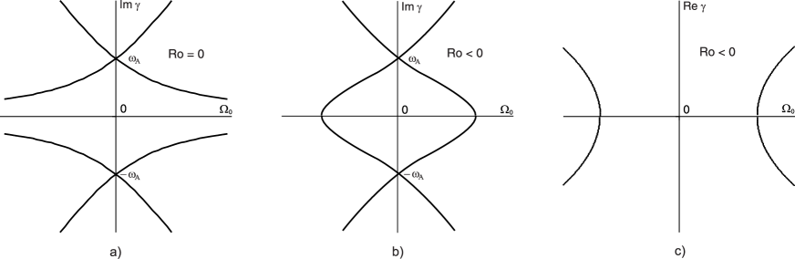
Figure 1: (a) Coriolis splitting of the Alfvén plane wave into the fast and the slow Magneto-Coriolis (MC) waves, (b) shear causes interaction of slow MC branches with the origination of the double zero eigenvalue, (c) splitting of the double zero eigenvalue yields positive real eigenvalues (SMRI).

The connection of SMRI and HMRI is presently under intense debate Liu et al. (2006); Rüdiger & Hollerbach (2007); Priede et al. (2007); Lakhin & Velikhov (2007); Liu et al. (2007); Szklarski (2007); Rüdiger & Schultz (2008); Liu (2009); Priede & Gerbeth (2009). The first essential point to note here is that HMRI and SMRI are connected. Indeed, Fig. 1 in Hollerbach & Rüdiger (2005) shows that there is a continuous and monotonic transition from HMRI to SMRI when ${\rm Re}$ and the magnetic field strength are increased simultaneously.

A second remarkable property of HMRI for small ${\rm Pm}$ (which has been coined “inductionless MRI”), was clearly worked out in Priede et al. (2007). It is the apparent paradox that a magnetic field is able to trigger an instability although the total energy dissipation of the system is larger than without this field.

The relevance of HMRI for Keplerian flows has been seriously put into question in Liu et al. (2006). Using a local WKB analysis in the small-gap approximation, the authors had shown that the HMRI works only for comparably steep rotation profiles (i.e. slightly above the Rayleigh line) and disappears for profiles as flat as the Keplerian one. This result has been confirmed by Lakhin and Velikhov Lakhin & Velikhov (2007) and Rüdiger and Schultz Rüdiger & Schultz (2008).

However, this disappointing result was soon relativized in Rüdiger & Hollerbach (2007) by solving the global eigenvalue equation for HMRI with electrical boundary conditions. It turned out that HMRI re-appears again for Keplerian flows provided that at least one radial boundary is highly conducting. A similar discrepancy between local and global results is well known for the so-called stratorotational instability (SRI) Dubrulle et al. (2005) for which the existence of reflecting boundaries appears necessary for the instability to work Umurhan (2006). This artificial demand is of course a much stronger argument against the working of SRI than the necessity of one conducting boundary is for the working of HMRI: considering, i.e., the colder outer parts of accretion disks, then the inner part can indeed be considered as a good conductor Balbus & Henri (2008).

Another argument that has been put forward against the relevance of HMRI for thin accretion disks is the necessity for a large ratio of toroidal to poloidal magnetic fields Liu (2008).

A further complication for applying HMRI to the real world is the fact that it appears in form of a travelling wave. The crucial point here is that monochromatic waves are typically not able to fulfill the axial boundary conditions at the ends of the considered region. To fulfill them, one has to consider wave packets. Only wave packets with vanishing group velocity will remain in the finite length system. Typically, the onset of this absolute instability, characterized by a zero growth rate and a zero group velocity, is harder to achieve than the convective instability of a monochromatic wave with zero growth rate. A comprehensive analysis of the relation of convective and absolute instability for HMRI can be found in Priede & Gerbeth (2009). From the extrapolation of the results of this paper it seems that Keplerian rotation profiles (with conducting boundaries) are indeed absolutely HMRI-unstable, but a final solution to this puzzle is still elusive.

In the present paper, we step back from those important consideration of absolute and global instabilities and focus again on the local WKB method by considering the dispersion relation of MRI which had been derived and analyzed in Liu et al. (2006); Lakhin & Velikhov (2007); Rüdiger & Schultz (2008). In spite of these former investigations, we feel that some points still need further clarification. This concerns a careful application of the Bilharz stability criterion as well as some further parameter dependencies, in particular the dependence for small but finite magnetic Prandtl numbers. It also concerns the question in which sense the HMRI can be considered as a dissipation induced instability which is quite common in many areas of physics Krechetnikov & Marsden (2007); Kirillov (2007).

To make the paper self-contained, we will start with a re-derivation of the dispersion relation in two forms which explicitly contain the relevant frequencies or the dimensionless parameters, respectively.

Then we will study the peculiar relation of SMRI and HMRI. As a main result of this paper we will describe in detail the mechanism of transition from SMRI to HMRI through a spectral exceptional point which appears at finite but small ${\rm Pm}$. This provides a natural explanation for the continuous and monotonic connection between SMRI (a destabilized slow magneto-Coriolis wave) and HMRI (a weakly destabilized inertial oscillation). In addition to this, for high Reynolds numbers we will identify a second scenario for HMRI which leads to new islands of instability at small but finite values of $\rm Pm$.

2 Mathematical setting

In order to make the paper self-contained, we will re-derive in this section the dispersion relation for HMRI, including viscosity and resistivity effects. Note that this dispersion relation was derived in various forms and approximations by a number of authors Liu et al. (2007); Lakhin & Velikhov (2007); Rüdiger et al. (2008).

The standard set of non-linear equations of dissipative incompressible magnetohydrodynamics (Ji et al., 2001; Goodman & Ji, 2002; Noguchi et al., 2002; Lakhin & Velikhov, 2007; Rüdiger & Schultz, 2008) consists of the Navier-Stokes equation for the fluid velocity ${\bf u}$

$$\frac{\partial{\bf u}}{\partial t}+({\bf u}\cdot\nabla){\bf u}=-\frac{1}{\rho}\nabla\left(p+\frac{{\bf B}^{2}}{2\mu_{0}}\right)+\frac{1}{\mu_{0}\rho}({\bf B}\cdot\nabla){\bf B}+\nu\nabla^{2}{\bf u},$$ (1)

and of the induction equation for the magnetic field ${\bf B}$

$$\frac{\partial{\bf B}}{\partial t}=\nabla\times({\bf u}\times{\bf B})+\eta\bigtriangledown^{2}{\bf B},$$ (2)

where $p$ is the pressure, $\rho=const$ the density, $\nu=const$ the kinematic viscosity, $\eta=(\mu_{0}\sigma)^{-1}$ the magnetic diffusivity, $\sigma$ the conductivity of the fluid, and $\mu_{0}$ the magnetic permeability of free space. Additionally, the mass continuity equation for incompressible flows and the solenoidal condition for the magnetic induction yield

$$\nabla\cdot{\bf u}=0,\quad\nabla\cdot{\bf B}=0.$$ (3)

We consider the rotational fluid flow in the gap between the radii $R_{1}$ and $R_{2}>R_{1}$, with an imposed magnetic field sustained by currents external to the fluid. The latter is important in order to distinguish the MRI from other instabilities (i.e. the Tayler instability for which electric currents are applied to the fluid). Introducing the cylindrical coordinates $(R,\phi,z)$ we consider the stability of a steady-state background liquid flow with the angular velocity profile $\Omega(R)$ in helical background magnetic field (a magnetized Taylor-Couette flow)

$${\bf u}_{0}=R\,\Omega(R)\,{\bf e}_{\phi},\quad p=p_{0}(R),\quad{\bf B}_{0}=B_{\phi}^{0}(R){\bf e}_{\phi}+B_{z}^{0}{\bf e}_{z},$$ (4)

with the azimuthal component

$$B_{\phi}^{0}(R)=\frac{\mu_{0}I}{2\pi R},$$ (5)

which can be thought as being produced by an axial current $I$. The angular velocity profile of the background TC flow is

$$\Omega(R)=a+\frac{b}{R^{2}},$$ (6)

where $a$ and $b$ are arbitrary constants as in Taylor-Couette experiments Wendl (1999). The centrifugal acceleration of the background flow (6) is compensated by the pressure gradient Ji et al. (2001)

$$R\Omega^{2}=\frac{1}{\rho}\frac{\partial p_{0}}{\partial R}.$$ (7)

2.1 Linearization with respect to axisymmetric perturbations

Throughout the paper we will restrict our interest to axisymmetric perturbations ${\bf u}^{\prime}={\bf u}^{\prime}(R,z)$, ${\bf B}^{\prime}={\bf B}^{\prime}(R,z)$, and ${p}^{\prime}={p}^{\prime}(R,z)$ about the stationary solution (4)-(7), keeping in mind that for strongly dominant azimuthal magnetic fields also non-axisymmetric perturbations are possible Hollerbach et al. (2009).

With the notation

$$D_{1}=\partial_{R}\partial_{R}^{\dagger}+\partial_{z}^{2},\quad D_{2}=\partial_{R}^{\dagger}\partial_{R}+\partial_{z}^{2},$$ (8)

where the differential operators are defined in (A1), the general linearized equations (A) derived in the

Appendix are simplified in the assumption of axisymmetric perturbations to

$$(\partial_{t}-\nu D_{1})u_{R}^{\prime}-2\Omega u_{\phi}^{\prime} = -\frac{1}{\rho}\left[\partial_{R}p^{\prime}+\frac{1}{\mu_{0}}\left(B_{z}^{0}{\partial_{R}}B_{z}^{\prime}+B_{\phi}^{0}{\partial_{R}}B_{\phi}^{\prime}\right)\right]+\frac{1}{\mu_{0}\rho}\left(B_{z}^{0}{\partial_{z}}B_{R}^{\prime}-\frac{B_{\phi}^{0}}{R}B_{\phi}^{\prime}\right),$$

$$({\partial_{t}}-\nu D_{1})u_{\phi}^{\prime}+\frac{\kappa^{2}}{2\Omega}u_{R}^{\prime} = \frac{B_{z}^{0}}{\mu_{0}\rho}{\partial_{z}B_{\phi}^{\prime}},$$

$$({\partial_{t}}-\nu D_{2})u_{z}^{\prime} = -\frac{1}{\rho}\left[{\partial_{z}p^{\prime}}+\frac{1}{\mu_{0}}\left(B_{z}^{0}{\partial_{z}B_{z}^{\prime}}+B_{\phi}^{0}{\partial_{z}B_{\phi}^{\prime}}\right)\right]+\frac{B_{z}^{0}}{\mu_{0}\rho}{\partial_{z}B_{z}^{\prime}},$$

$$({\partial_{t}}-\eta D_{1})B_{R}^{\prime} = B_{z}^{0}{\partial_{z}u_{R}^{\prime}},$$

$$({\partial_{t}}-\eta D_{1})B_{\phi}^{\prime} = B_{z}^{0}{\partial_{z}u_{\phi}^{\prime}}+\frac{2B_{\phi}^{0}}{R}u_{R}^{\prime}+(R{\partial_{R}\Omega})B_{R}^{\prime},$$

$$({\partial_{t}}-\eta D_{2})B_{z}^{\prime} = -B_{z}^{0}\partial_{R}^{\dagger}u_{R}^{\prime},$$

$${\partial_{z}u_{z}^{\prime}} = -\partial_{R}^{\dagger}u_{R}^{\prime},$$

$${\partial_{z}B_{z}^{\prime}} = -\partial_{R}^{\dagger}B_{R}^{\prime},$$ (9)

where the squared epicyclic frequency $\kappa$ is defined as

$$\kappa^{2}=2\Omega\left(2\Omega+R\frac{d\Omega}{dR}\right)=\frac{1}{R^{3}}\frac{d}{dR}(\Omega^{2}R^{4}).$$ (10)

Following the approach of Goodman & Ji (2002); Liu et al. (2006) we act on the first of equations (2.1) by the operator $\partial_{R}^{\dagger}$ and on the third one by the operator $\partial_{z}$. Summing the results, taking into account that

$$\partial_{R}^{\dagger}D_{1}=D_{2}\partial_{R}^{\dagger},\quad\partial_{R}^{\dagger}B_{\phi}^{0}=0,\quad\partial_{R}(B_{\phi}^{0}B_{\phi}^{\prime})=-\frac{B_{\phi}^{0}B_{\phi}^{\prime}}{R}+B_{\phi}^{0}\partial_{R}B_{\phi}^{\prime},$$ (11)

and using the last two equations of (2.1) yields

$$-2\Omega\partial_{R}^{\dagger}u_{\phi}^{\prime} = -\frac{1}{\rho}D_{2}\left[p^{\prime}+\frac{1}{\mu_{0}}B_{z}^{0}B_{z}^{\prime}\right]-\frac{1}{\rho}\frac{1}{\mu_{0}}(\partial_{R}^{\dagger}B_{\phi}^{0}\partial_{R}+\partial_{z}^{2}B_{\phi}^{0})B_{\phi}^{\prime}-\frac{1}{\mu_{0}\rho}\partial_{R}^{\dagger}\left(\frac{B_{\phi}^{0}}{R}B_{\phi}^{\prime}\right)$$ (12)

$$= -\frac{1}{\rho}D_{2}\left[p^{\prime}+\frac{1}{\mu_{0}}(B_{z}^{0}B_{z}^{\prime}+B_{\phi}^{0}B_{\phi}^{\prime})\right]-\frac{2}{\mu_{0}\rho}\partial_{R}^{\dagger}\left(\frac{B_{\phi}^{0}}{R}B_{\phi}^{\prime}\right).$$

Therefore, we extend the identity obtained in Goodman & Ji (2002) to the case $B_{\phi}^{0}\neq 0$

$$D_{2}\frac{1}{\rho}\left[p^{\prime}+\frac{1}{\mu_{0}}(B_{z}^{0}B_{z}^{\prime}+B_{\phi}^{0}B_{\phi}^{\prime})\right]=2\partial_{R}^{\dagger}\left(\Omega u_{\phi}^{\prime}-\frac{1}{\mu_{0}\rho}\frac{B_{\phi}^{0}}{R}B_{\phi}^{\prime}\right).$$ (13)

On the other hand, using (11) we transform the first of the equations (2.1) into

$$(\partial_{t}-\nu D_{1})u_{R}^{\prime}-2\Omega u_{\phi}^{\prime} = -\partial_{R}\frac{1}{\rho}\left[p^{\prime}+\frac{1}{\mu_{0}}\left(B_{z}^{0}B_{z}^{\prime}+B_{\phi}^{0}B_{\phi}^{\prime}\right)\right]$$ (14)

$$+ \frac{1}{\mu_{0}\rho}\left(B_{z}^{0}{\partial_{z}}B_{R}^{\prime}-\frac{2B_{\phi}^{0}}{R}B_{\phi}^{\prime}\right).$$

Acting on both sides of the equation (14) by the operator $D_{1}$ and taking into account the identity (13) and

$$D_{1}\partial_{R}=(\partial_{R}\partial_{R}^{\dagger}+\partial_{z}^{2})\partial_{R}=\partial_{R}(\partial_{R}^{\dagger}\partial_{R}+\partial_{z}^{2})=\partial_{R}D_{2}$$ (15)

we get

$$D_{1}(\partial_{t}-\nu D_{1})u_{R}^{\prime} - 2\Omega D_{1}u_{\phi}^{\prime}$$ (16)

$$= -\partial_{R}D_{2}\frac{1}{\rho}\left[p^{\prime}+\frac{1}{\mu_{0}}\left(B_{z}^{0}B_{z}^{\prime}+B_{\phi}^{0}B_{\phi}^{\prime}\right)\right]+D_{1}\frac{1}{\mu_{0}\rho}\left(B_{z}^{0}{\partial_{z}}B_{R}^{\prime}-\frac{2B_{\phi}^{0}}{R}B_{\phi}^{\prime}\right)$$

$$= -2\partial_{R}\partial_{R}^{\dagger}\left(\Omega u_{\phi}^{\prime}-\frac{1}{\mu_{0}\rho}\frac{B_{\phi}^{0}}{R}B_{\phi}^{\prime}\right)+D_{1}\frac{1}{\mu_{0}\rho}\left(B_{z}^{0}{\partial_{z}}B_{R}^{\prime}-\frac{2B_{\phi}^{0}}{R}B_{\phi}^{\prime}\right).$$

Rearranging the terms and using the definition of the operator $D_{1}$ yields

$$D_{1}(\partial_{t}-\nu D_{1})u_{R}^{\prime}-2\Omega\partial_{z}^{2}u_{\phi}^{\prime} = 2\partial_{R}\partial_{R}^{\dagger}\frac{1}{\mu_{0}\rho}\frac{B_{\phi}^{0}}{R}B_{\phi}^{\prime}+\frac{1}{\mu_{0}\rho}B_{z}^{0}D_{1}{\partial_{z}}B_{R}^{\prime}-\frac{1}{\mu_{0}\rho}D_{1}\frac{2B_{\phi}^{0}}{R}B_{\phi}^{\prime}$$ (17)

$$= \frac{1}{\mu_{0}\rho}B_{z}^{0}D_{1}{\partial_{z}}B_{R}^{\prime}-\frac{1}{\mu_{0}\rho}\frac{2B_{\phi}^{0}}{R}\partial_{z}^{2}B_{\phi}^{\prime}.$$

Therefore, we have separated the equations for $u_{R}^{\prime}$, $u_{\phi}^{\prime}$ and $B_{R}^{\prime}$, $B_{\phi}^{\prime}$ from the others in (2.1)

$$(\partial_{t}-\nu D_{1})D_{1}u_{R}^{\prime}-2\Omega\partial_{z}^{2}u_{\phi}^{\prime} = \frac{1}{\mu_{0}\rho}B_{z}^{0}D_{1}{\partial_{z}}B_{R}^{\prime}-\frac{1}{\mu_{0}\rho}\frac{2B_{\phi}^{0}}{R}\partial_{z}^{2}B_{\phi}^{\prime},$$

$$({\partial_{t}}-\nu D_{1})u_{\phi}^{\prime}+\frac{\kappa^{2}}{2\Omega}u_{R}^{\prime} = \frac{B_{z}^{0}}{\mu_{0}\rho}{\partial_{z}B_{\phi}^{\prime}},$$

$$({\partial_{t}}-\eta D_{1})B_{R}^{\prime} = B_{z}^{0}{\partial_{z}u_{R}^{\prime}},$$

$$({\partial_{t}}-\eta D_{1})B_{\phi}^{\prime} = B_{z}^{0}{\partial_{z}u_{\phi}^{\prime}}+\frac{2B_{\phi}^{0}}{R}u_{R}^{\prime}+(R{\partial_{R}\Omega})B_{R}^{\prime}.$$ (18)

Note that after introducing the stream functions for the poloidal components

$$u_{R}^{\prime}=\partial_{z}\varphi,\quad u_{z}^{\prime}=-\partial_{R}^{\dagger}\varphi,\quad B_{R}^{\prime}=\partial_{z}\psi,\quad B_{z}^{\prime}=-\partial_{R}^{\dagger}\psi,$$ (19)

the equations (2.1) extend the inviscid equations of Liu et al. (2006) to the case $\nu\neq 0$.

We can rewrite (2.1) in the form of the operator matrix equation $\partial_{t}\tilde{E}\xi^{\prime}=\tilde{H}\xi^{\prime}$, where $\xi^{\prime}=(u_{R}^{\prime},u_{\phi}^{\prime},B_{R}^{\prime},B_{\phi}^{\prime})^{T}$,

$$\tilde{E}=\left(\begin{array}[]{cccc}D_{1}&0&0&0\\ 0&1&0&0\\ 0&0&1&0\\ 0&0&0&1\\ \end{array}\right),\quad\tilde{H}=\left(\begin{array}[]{cccc}\nu D_{1}^{2}&2\Omega\partial_{z}^{2}&\frac{B_{z}^{0}}{\mu_{0}\rho}D_{1}{\partial_{z}}&-\frac{2B_{\phi}^{0}}{\mu_{0}\rho R}\partial_{z}^{2}\\ -\frac{\kappa^{2}}{2\Omega}&\nu D_{1}&0&\frac{B_{z}^{0}}{\mu_{0}\rho}{\partial_{z}}\\ B_{z}^{0}\partial_{z}&0&\eta D_{1}&0\\ \frac{2B_{\phi}^{0}}{R}&B_{z}^{0}\partial_{z}&R{\partial_{R}\Omega}&\eta D_{1}\\ \end{array}\right).$$ (20)

The resulting multiparameter family of operator matrices equipped with boundary conditions can be investigated by numerical or perturbative Kirillov (2010) methods. In the following we use the local WKB approximation.

2.2 Local WKB approximation

We choose a fiducial point $(R_{0},z_{0})$, around which we perform the local stability analysis Pessah & Psaltis (2005). We expand all the background quantities in Taylor series around $(R_{0},z_{0})$ and retain only the zeroth order in terms of the local coordinates $\tilde{R}=R-R_{0}$ and $\tilde{z}=z-z_{0}$ to obtain the operator matrix equation with the constant coefficients

$$\partial_{t}\tilde{E}_{0}\xi^{\prime}=\tilde{H}_{0}\xi^{\prime}$$ (21)

with

$$\tilde{E}_{0}=\left(\begin{array}[]{cccc}D_{1}^{0}&0&0&0\\ 0&1&0&0\\ 0&0&1&0\\ 0&0&0&1\\ \end{array}\right),\quad\tilde{H}_{0}=\left(\begin{array}[]{cccc}\nu({D_{1}^{0}})^{2}&2\Omega_{0}\partial_{\tilde{z}}^{2}&\frac{B_{z}^{0}}{\mu_{0}\rho}D_{1}^{0}{\partial_{\tilde{z}}}&-\frac{2B_{\phi}^{0}}{\mu_{0}\rho R_{0}}\partial_{\tilde{z}}^{2}\\ -\frac{\kappa_{0}^{2}}{2\Omega_{0}}&\nu D_{1}^{0}&0&\frac{B_{z}^{0}}{\mu_{0}\rho}{\partial_{\tilde{z}}}\\ B_{z}^{0}\partial_{\tilde{z}}&0&\eta D_{1}^{0}&0\\ \frac{2B_{\phi}^{0}}{R_{0}}&B_{z}^{0}\partial_{\tilde{z}}&\frac{\kappa_{0}^{2}}{2\Omega_{0}}-2\Omega_{0}&\eta D_{1}^{0}\\ \end{array}\right),$$ (22)

where

$$\Omega_{0}=\Omega(R_{0}),\quad\kappa_{0}^{2}=2\Omega_{0}\left(2\Omega_{0}+R_{0}\left.\frac{d\Omega}{dR}\right|_{R=R_{0}}\right),\quad B_{\phi}^{0}=B_{\phi}^{0}(R_{0}),\quad D_{1}^{0}=\partial_{\tilde{R}}^{2}+\partial_{\tilde{z}}^{2}+\frac{\partial_{\tilde{R}}}{R_{0}}-\frac{1}{R_{0}^{2}}.$$ (23)

Equation (21) is a linear PDE with the constant coefficients in the local variables $(\tilde{R},\tilde{z})$ for the perturbed quantities $\xi^{\prime}$. This is a good approximation as long as the variations $\tilde{R}$ and $\tilde{z}$ are small in comparison with the characteristic length scales in the radial and vertical directions, respectively Pessah & Psaltis (2005). A solution to the equation (21) has the form of a plane wave

$${\xi}^{\prime} = \tilde{\xi}\exp{(\gamma t+ik_{R}\tilde{R}+ik_{z}\tilde{z})},\quad\tilde{\xi}=(\tilde{u}_{R},\tilde{u}_{\phi},\tilde{B}_{R},\tilde{B}_{\phi})^{T},$$ (24)

where $\tilde{\xi}$ is a vector of constant coefficients.

Introducing the total wave number $k^{2}=k_{z}^{2}+k_{R}^{2}$ and denoting $\alpha=k_{z}/k$, we find

$$D_{1}^{0}\exp{(\gamma t+ik_{R}\tilde{R}+ik_{z}\tilde{z})} = \left(-k^{2}+\frac{ik_{R}}{R_{0}}-\frac{1}{R_{0}^{2}}\right)\exp{(\gamma t+ik_{R}\tilde{R}+ik_{z}\tilde{z})}.$$ (25)

In the WKB approximation we restrict the analysis to the modes with the wave numbers satisfying $k_{R}R_{0}\gg 1$ which allows us to neglect the terms $\frac{ik_{R}}{R_{0}}-\frac{1}{R_{0}^{2}}$ in (25). In view of this, after substitution of (24) into equation (21), we arrive at the matrix eigenvalue problem

$$(H-\gamma E)\tilde{\xi}=0,$$ (26)

with $E$ as a unit matrix and $H=-{\rm diag}(\omega_{\nu},\omega_{\nu},\omega_{\eta},\omega_{\eta})+H_{1}+H_{2}$, where $\omega_{\nu}=\nu k^{2}$ and $\omega_{\eta}=\eta k^{2}$ are the viscous and resistive frequencies,

$$H_{1}=\frac{i\omega_{A}}{\sqrt{\mu_{0}\rho}}\left(\begin{array}[]{cccc}0&0&1&0\\ 0&0&0&1\\ \mu_{0}\rho&0&0&0\\ 0&\mu_{0}\rho&0&0\\ \end{array}\right),$$ (27)

$$H_{2}=\left(\begin{array}[]{cccc}0&2\Omega_{0}\alpha^{2}&0&-2\omega_{A_{\phi}}\frac{\alpha^{2}}{\sqrt{\mu_{0}\rho}}\\ -2\Omega_{0}-R_{0}\left.\frac{d\Omega}{dR}\right|_{R=R_{0}}&0&0&0\\ 0&0&0&0\\ -2\omega_{A_{\phi}}{\sqrt{\mu_{0}\rho}}&0&R_{0}\left.\frac{d\Omega}{dR}\right|_{R=R_{0}}&0\\ \end{array}\right),$$ (28)

and the Alfvén frequencies are

$$\omega_{A}^{2}=\frac{k_{z}^{2}(B_{z}^{0})^{2}}{\mu_{0}\rho},\quad\omega_{A_{\phi}}^{2}=\frac{(B_{\phi}^{0})^{2}}{\mu_{0}\rho R_{0}^{2}}.$$ (29)

Note that the matrix $-{\rm diag}(\omega_{\nu},\omega_{\nu},\omega_{\eta},\omega_{\eta})+H_{1}$ has two double eigenvalues related to the damped Alfvén modes Nornberg et al. (2009)

$$\gamma_{1,2}=-\frac{\omega_{\nu}+\omega_{\eta}}{2}+\sqrt{\left(\frac{\omega_{\nu}-\omega_{\eta}}{2}\right)^{2}-\omega_{A}^{2}},\quad\gamma_{3,4}=-\frac{\omega_{\nu}+\omega_{\eta}}{2}-\sqrt{\left(\frac{\omega_{\nu}-\omega_{\eta}}{2}\right)^{2}-\omega_{A}^{2}}.$$ (30)

When $\omega_{A_{\phi}}=0$, $\left.\frac{d\Omega}{dR}\right|_{R=R_{0}}=0$, the eigenvalues of the matrix $H_{1}+H_{2}$ correspond to the Alfvén-inertial or Magneto-Coriolis waves Lehnert (1954)

$$\gamma_{1,2}=i\sqrt{\omega_{A}^{2}+\Omega_{0}^{2}\alpha^{2}}\pm i\alpha\Omega_{0},\quad\gamma_{3,4}=-i\sqrt{\omega_{A}^{2}+\Omega_{0}^{2}\alpha^{2}}\pm i\alpha\Omega_{0}.$$ (31)

Figure 1 demonstrates how rotation leads to the splitting of plane Alfvén waves into the fast and slow Magneto-Coriolis waves Lehnert (1954). The system with purely imaginary eigenvalues (31) is marginally stable and its destabilization caused by dissipative, shear, and azimuthal magnetic field perturbations admits thus a natural interpretation as a dissipation-induced instability Krechetnikov & Marsden (2007); Kirillov (2007, 2009).

On the other hand, the matrix $H$ can be considered as a result of a non-Hermitian complex perturbation $H_{1}+H_{2}$ of a real symmetric matrix, which has two double semi-simple eigenvalues—diabolical points Berry & Dennis (2003). This is a typical situation for the problems of wave propagation in chiral absorptive media Keck et al. (2003); Berry & Dennis (2003); Kirillov et al. (2005) or in rotating symmetric continua Kirillov (2009).

2.3 Dispersion relation in terms of dimensionless parameters

The stability of the propagating plane wave perturbation (25) is determined by the roots $\gamma$ of the dispersion relation $P(\gamma)=\det(H-\gamma E)=0$, where

$$P(\gamma)=\gamma^{4}+a_{1}\gamma^{3}+a_{2}\gamma^{2}+(a_{3}+ib_{3})\gamma+a_{4}+ib_{4}=0.$$ (32)

We write the coefficients of the complex polynomial (32) in the form

$$a_{1} = 2(\omega_{\nu}+\omega_{\eta}),$$

$$a_{2} = (\omega_{\nu}+\omega_{\eta})^{2}+2(\omega_{A}^{2}+\omega_{\nu}\omega_{\eta})+\alpha^{2}\kappa_{0}^{2}+4\alpha^{2}\omega_{A_{\phi}}^{2},$$

$$a_{3} = 2(\omega_{\eta}+\omega_{\nu})(\omega_{A}^{2}+\omega_{\eta}\omega_{\nu})+2\alpha^{2}\kappa_{0}^{2}\omega_{\eta}+4\alpha^{2}(\omega_{\eta}+\omega_{\nu})\omega^{2}_{A_{\phi}},$$

$$a_{4} = (\omega_{A}^{2}+\omega_{\nu}\omega_{\eta})^{2}-4\alpha^{2}\omega_{A}^{2}\Omega_{0}^{2}+\alpha^{2}\kappa_{0}^{2}(\omega_{A}^{2}+\omega_{\eta}^{2})+4\alpha^{2}\omega_{\nu}\omega_{\eta}\omega_{A_{\phi}}^{2},$$

$$b_{3} = -8\alpha^{2}\Omega_{0}\omega_{A}\omega_{A_{\phi}},$$

$$b_{4} = -4\alpha^{2}\Omega_{0}\omega_{A}\omega_{A_{\phi}}(2\omega_{\eta}+\omega_{\nu})-\kappa_{0}^{2}\alpha^{2}\Omega_{0}^{-1}\omega_{A}\omega_{A_{\phi}}(\omega_{\eta}-\omega_{\nu}).$$ (33)

After scaling the spectral parameter as $\gamma=\lambda\sqrt{\omega_{\nu}\omega_{\eta}}$, we express the appropriately normalized coefficients (2.3) by means of the dimensionless Rossby number $({\rm Ro})$, magnetic Prandtl number $({\rm Pm})$, ratio of the Alfvén frequencies $(\beta^{*})$, Hartmann $({\rm Ha}^{*})$, and Reynolds $({\rm Re}^{*})$ numbers

$${\rm Ro}=\frac{1}{2}\frac{R_{0}}{\Omega_{0}}\left.\frac{d\Omega}{dR}\right|_{R=R_{0}},\quad{\rm Pm}=\frac{\nu}{\eta}=\frac{\omega_{\nu}}{\omega_{\eta}},\quad\beta^{*}=\alpha\frac{\omega_{A_{\phi}}}{\omega_{A}},\quad{\rm Re^{*}}=\alpha\frac{\Omega_{0}}{\omega_{\nu}},\quad{{\rm Ha}^{*}}=\alpha\frac{B_{z}^{0}}{k\sqrt{\mu_{0}\rho\nu\eta}}.$$ (34)

Additional transformation yields the coefficients of the dispersion relation $P(\lambda)=0$ in a simplified form

$$a_{1} = 2\left(\sqrt{\rm Pm}+\frac{1}{\sqrt{\rm Pm}}\right),$$

$$a_{2} = \frac{a_{1}^{2}}{4}+2({1+{\rm Ha}^{*}}^{2})+4{\beta^{*}}^{2}{{\rm Ha}^{*}}^{2}+4{\rm Re^{*}}^{2}{\rm Pm}(1+{\rm Ro}),$$

$$a_{3} = a_{1}(1+{{\rm Ha}^{*}}^{2})+2a_{1}{\beta^{*}}^{2}{{\rm Ha}^{*}}^{2}+8{{\rm Re}^{*}}^{2}(1+{\rm Ro})\sqrt{\rm Pm},$$

$$a_{4} = \left(1+{{\rm Ha}^{*}}^{2}\right)^{2}+4{\beta^{*}}^{2}{{\rm Ha}^{*}}^{2}+4{\rm Re^{*}}^{2}+4{\rm Re^{*}}^{2}{\rm Ro}({\rm Pm}{{\rm Ha}^{*}}^{2}+1),$$

$$b_{3} = -8\beta^{*}{{\rm Ha}^{*}}^{2}{\rm Re}^{*}\sqrt{\rm Pm},$$

$$b_{4} = -4\beta^{*}{{\rm Ha}^{*}}^{2}{\rm Re}^{*}(2+(1-{\rm Pm}){\rm Ro}).$$ (35)

Therefore, we have exactly reproduced the dispersion relation of Lakhin & Velikhov (2007); Rüdiger & Schultz (2008), which generalizes that of Goodman & Ji (2002); Liu et al. (2006).

3 SMRI in the absence of the azimuthal magnetic field $(\beta^{*}=0)$

Let us first assume $\beta^{*}=0$ and study the onset of the standard magnetorotational instability (SMRI). The coefficients of the polynomial $P(\lambda)$ are then real because $b_{3}=0$ and $b_{4}=0$. We have

$$a_{1} = \hat{a}_{1}=2\left(\sqrt{\rm Pm}+\frac{1}{\sqrt{\rm Pm}}\right),$$

$$a_{2} = \hat{a}_{2}=\frac{\hat{a}_{1}^{2}}{4}+2({1+{\rm Ha}^{*}}^{2})+4{\rm Re^{*}}^{2}{\rm Pm}(1+{\rm Ro}),$$

$$a_{3} = \hat{a}_{3}=\hat{a}_{1}(1+{{\rm Ha}^{*}}^{2})+8{{\rm Re}^{*}}^{2}(1+{\rm Ro})\sqrt{\rm Pm},$$

$$a_{4} = \hat{a}_{4}=\left(1+{{\rm Ha}^{*}}^{2}\right)^{2}+4{\rm Re^{*}}^{2}(1+{\rm Ro}({\rm Pm}{{\rm Ha}^{*}}^{2}+1)).$$ (36)

Composing the Hurwitz matrix of the real polynomial $P(\lambda)$ we write the Lienard and Chipart criterion of asymptotic stability Lienard & Chipart (1914); Marden (1966): all roots $\lambda$ have ${\rm Re}\lambda<0$ if and only if

$$\hat{a}_{4}>0,\quad\hat{a}_{2}>0,\quad h_{1}=\hat{a}_{1}>0,\quad h_{3}=\hat{a}_{1}\hat{a}_{1}\hat{a}_{3}-\hat{a}_{1}^{2}\hat{a}_{4}-\hat{a}_{3}^{2}>0.$$ (37)

Explicit calculation of $h_{3}$ shows that it is a sum of squared quantities

$$h_{3}=64\left({\rm Pm^{*}}{\rm Re^{*}}^{2}({\rm Ro}+1)+\frac{\hat{a}_{1}^{2}}{16}\right)^{2}+{\rm Ha^{*}}^{2}\hat{a}_{1}^{2}\left(\frac{\hat{a}_{1}^{2}}{4}+4{\rm Re^{*}}^{2}\right)>0$$ (38)

Therefore, the condition $h_{3}>0$ is always fulfilled.

The local definition of the Rossby number (34) allows us to vary it for the background profile $\Omega(R)=a+bR^{-2}$ changing the coefficients $a$ and $b$ because ${\rm Ro}=-b/(aR_{0}^{2}+b)$. On the other hand we can interpret the Rossby numbers as if they would correspond to quite general rotation profiles $\Omega(R)$, which can have, e.g., the shape $\Omega(R)\sim R^{w}$ (with $w=-3/2$ and ${\rm Ro}=w/2=-3/4$ for Kepler rotation).

In the following we assume ${\rm Ro}\geq-1$ that corresponds to the centrifugally (Rayleigh) stable flow in the absence of the magnetic field. This reduces the conditions (37) to $\hat{a}_{4}>0$ that is equivalent to

$${\rm Ro}>{\rm Ro}^{c}=-\frac{\left(1+{\rm Ha^{*}}^{2}\right)^{2}+4{\rm Re^{*}}^{2}}{4{\rm Re^{*}}^{2}({\rm Pm}{\rm Ha^{*}}^{2}+1)}.$$ (39)

Note that in the absence of the magnetic field, ${\rm Ha^{*}}=0$, the inequality (39) is

$${\rm Ro}>{\rm Ro}^{v}=-1-\frac{1}{4{\rm Re^{*}}^{2}},$$ (40)

where we define the viscous Rayleigh line ${\rm Ro}^{v}$. In the inviscid limit ${\rm Re}^{*}\rightarrow\infty$ it is reduced to the Rayleigh’s centrifugal stability criterion

$${\rm Ro}>{\rm Ro}^{i}=-1,$$ (41)

where ${\rm Ro}^{i}$ is the classical inviscid Rayleigh line.

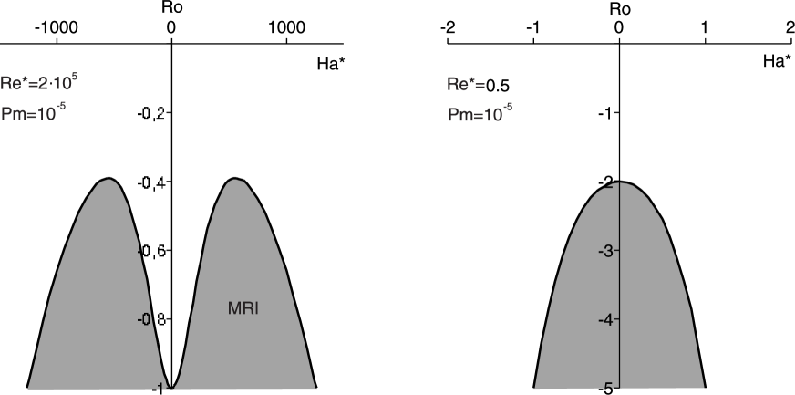
Figure 2: The domain according to equation (39) of the standard MRI (grey) for ${\rm Pm}=10^{-5}$ and (left) ${\rm Re}^{*}=2\cdot 10^{5}$ or (right) ${\rm Re}^{*}=0.5$. The left plot shows the typical SMRI peaks Ji et al. (2001).

As is seen in the Figure 2(left), there are two extrema of the function ${\rm Ro}^{c}({\rm Ha}^{*})$ at

$${\rm Ha^{*}}_{\max}=\pm\sqrt{\frac{-1+\sqrt{(1-{\rm Pm})^{2}+4{\rm Pm}^{2}{\rm Re^{*}}^{2}}}{\rm Pm}},$$ (42)

which agrees with the results of Ji et al. (2001). Triggered by the vertical magnetic field $(B_{z}^{0}\neq 0)$ at some values of ${\rm Ha}^{*}$ the flow becomes unstable for ${\rm Ro}>-1$. It can be stabilized again, however, with the further increase of ${\rm Ha}^{*}$, which is a hallmark of the standard MRI, cf. with Figure 1 in Ji et al. (2001).

The maximal values of the Rossby number at the peaks of the boundary of the SMRI domain are

$${\rm Ro}_{\max}^{c}=-\frac{4{\rm Re^{*}}^{2}{\rm Pm}^{2}+\left({\rm Pm}-1+\sqrt{(1-{\rm Pm})^{2}+4{\rm Re^{*}}^{2}{\rm Pm}^{2}}\right)^{2}}{4{\rm Re^{*}}^{2}{\rm Pm}^{2}\sqrt{(1-{\rm Pm})^{2}+4{\rm Re^{*}}^{2}{\rm Pm}^{2}}}.$$ (43)

The two extrema at ${\rm Ha^{*}}_{\max}\neq 0$ exist when the radicand in (42) is positive, that is when

$${\rm Re^{*}}{\rm Pm}>\frac{\sqrt{(2-{\rm Pm}){\rm Pm}}}{2}.$$ (44)

Otherwise, the unique maximum is at the origin, Figure 2(right). This condition also follows from the positiveness of the second-order coefficient in the series expansion of ${\rm Ro}^{c}({\rm Ha^{*}})$ at ${\rm Ha^{*}}=0$:

$${\rm Ro}^{c}=-\frac{1+4{\rm Re^{*}}^{2}}{4{\rm Re^{*}}^{2}}-\frac{2-(4{\rm Re^{*}}^{2}+1){\rm Pm}}{4{\rm Re^{*}}^{2}}{\rm Ha^{*}}^{2}+\cdots$$ (45)

Setting ${\rm Ro}_{\max}^{c}\geq-3/4$, we find the conditions for existence of the standard MRI at and above the Kepler line in terms of the magnetic Reynolds number ${\rm Rm}^{*}={\rm Re^{*}Pm}$

$${\rm Rm}^{*}\geq\frac{2}{3}\sqrt{1+3{\rm Pm}}.$$ (46)

For ${\rm Pm}\ll 1$ one should have ${\rm Rm}^{*}\geq 2/3$ to have SMRI for the Kepler flows, which leads to ${\rm Re^{*}}\gg 1$. At such values of $\rm Re^{*}$ the following formal asymptotic expansions of ${\rm Ha^{*}}_{\max}({\rm Re^{*}})$ and ${\rm Ro}_{\max}^{c}({\rm Re^{*}})$ are valid

$${\rm Ha^{*}}_{\max}=\pm\sqrt{2\rm Re^{*}}\mp\frac{\sqrt{2}}{4{\rm Pm}\sqrt{\rm Re^{*}}},\quad{\rm Ro}_{\max}^{c}=-\frac{1}{\rm PmRe^{*}}+\frac{1-{\rm Pm}}{2{\rm Pm}^{2}{\rm Re^{*}}^{2}}-\frac{(1-{\rm Pm})^{2}}{2^{3}{\rm Pm}^{3}{\rm Re^{*}}^{3}}.$$ (47)

The asymptotic expansion (47) gives a simple scaling law which is known to be a characteristic of SMRI

$${\rm Re^{*}}=\frac{1}{2}{\rm Ha^{*}}^{2}.$$ (48)

This equation is identical to $\rm N^{*}:={\rm Ha^{*}}^{2}/{\rm Re^{*}}=2$ where $\rm N^{*}$ is often called interaction parameter (in technical magnetohydrodynamics) or Elsasser number (in geo- and astrophysics).

The SMRI can be interpreted as destabilization of slow Magneto-Coriolis waves Nornberg (2008); Nornberg et al. (2009). Indeed in the presence of shear, ${\rm Ro}\neq 0$, we find from the equation (32) with the coefficients (2.3) that in the absence of dissipation ($\omega_{\nu}=0$, $\omega_{\eta}=0$) the eigenvalues are

$$\gamma=\pm\sqrt{-2\Omega_{0}^{2}\alpha^{2}(1+{\rm Ro})-\omega_{A}^{2}\pm 2\Omega_{0}\alpha\sqrt{\Omega_{0}^{2}\alpha^{2}(1+{\rm Ro})^{2}+\omega_{A}^{2}}}.$$ (49)

At the critical value $\Omega_{0}=\Omega_{0}^{c}$, where

$$\Omega_{0}^{c}=-\frac{\omega_{A}^{2}}{2\alpha^{2}R_{0}\partial_{R}\Omega},$$ (50)

the branches of the slow magnetic-Coriolis waves merge with the origination of the double zero eigenvalue, see Figure 1(b). Splitting of this eigenvalue yields positive real eigenvalues, see Figure 1(c). Note that the SMRI threshold (50) is equivalent to

$${\rm Ro}=-\frac{{\rm Ha^{*}}^{2}}{4{\rm Re^{*}}^{2}{\rm Pm}}$$ (51)

that follows from (39) when ${\rm Ha^{*}}\rightarrow\infty$.

4 HMRI in the presence of an azimuthal magnetic field $(\beta^{*}\neq 0)$

The fact that an additional azimuthal field changes the character of the MRI drastically had been detected by Knobloch as early as 1992 Knobloch (1992). He had shown that in this case the instability appears in form of a travelling wave (see also Knobloch (1996)). However, the difference in the scaling behaviour for small $\rm Pm$ between standard and helical MRI was worked out only recently Hollerbach & Rüdiger (2005), and is still the subject of intense debate. In this section we will contribute to this discussion by focusing on the specific $\rm Pm$ dependence of the helical MRI.

4.1 Bilharz criterion for asymptotic stability

With the appearance of the azimuthal magnetic field $(\beta^{*}\neq 0)$, the coefficients of the polynomial $P(\lambda)$ become complex. This breaks the symmetry of the eigenvalues with respect to the real axis of the complex plane and consequently may lead to dramatic changes in the stability properties of the system.

In contrast to previous studies Lakhin & Velikhov (2007); Rüdiger & Schultz (2008) that were based on the study of approximations to the roots of the dispersion relation

$$P(\lambda)=\lambda^{4}+a_{1}\lambda^{3}+a_{2}\lambda^{2}+(a_{3}+ib_{3})\lambda+a_{4}+ib_{4}=0,$$ (52)

we prefer to use the Bilharz criterion Bilharz (1944); Marden (1966) of asymptotic stability of the roots of complex polynomials. This criterion establishes the necessary and sufficient conditions for all the roots to be in the left part of the complex plane $({\rm Re}\lambda<0)$ in terms of positiveness of the main even-ordered minors of the Bilharz matrix. For the polynomial $P(\lambda)$ with the coefficients (2.3) this matrix is

$$B=\left(\begin{array}[]{cccccccc}a_{4}&-b_{4}&0&0&0&0&0&0\\ b_{3}&a_{3}&a_{4}&-b_{4}&0&0&0&0\\ -a_{2}&0&b_{3}&a_{3}&a_{4}&-b_{4}&0&0\\ 0&-a_{1}&-a_{2}&0&b_{3}&a_{3}&a_{4}&-b_{4}\\ 1&0&0&-a_{1}&-a_{2}&0&b_{3}&a_{3}\\ 0&0&1&0&0&-a_{1}&-a_{2}&0\\ 0&0&0&0&1&0&0&-a_{1}\\ 0&0&0&0&0&0&1&0\\ \end{array}\right).$$ (53)

The Bilharz stability conditions Bilharz (1944); Marden (1966) require positiveness of all diagonal even-ordered minors of $B$

$$m_{1} = a_{3}a_{4}+b_{3}b_{4}>0,$$ (54)

$$m_{2} = (a_{2}a_{3}-a_{1}a_{4})m_{1}-a_{2}^{2}b_{4}^{2}>0,$$

$$m_{3} = (a_{1}a_{2}-a_{3})m_{2}-(a_{1}^{2}a_{4}a_{2}+(a_{1}b_{3}-b_{4})^{2})m_{1}+a_{1}a_{4}(b_{4}a_{2}(2b_{4}-a_{1}b_{3})+a_{1}^{2}a_{4}^{2})>0,$$

$$m_{4} = a_{1}m_{3}-a_{1}a_{3}m_{2}+(a_{3}^{3}+a_{1}^{2}b_{4}b_{3}-2a_{1}b_{4}^{2})m_{1}+a_{1}b_{4}^{2}a_{4}(a_{1}a_{2}-a_{3})-b_{4}^{2}a_{3}^{2}a_{2}+b_{4}^{4}>0.$$

The inequalities (54) determine the stability condition of the general dispersion relation (52) in the presence of both vertical $(B_{z}^{0})$ and azimuthal $(B_{\phi}^{0})$ components of the magnetic field.

We first note that for $\beta^{*}=0$ the stability conditions (54) are reduced to the stability condition $\hat{a}_{4}>0$ that was derived in the previous section. Indeed, with $\beta^{*}=0$ the coefficients $b_{3}$ and $b_{4}$ vanish to zero, which yields

$$m_{1}=\hat{a}_{4}\hat{a}_{3},\quad m_{2}=\hat{a}_{4}\hat{a}_{3}(\hat{a}_{2}\hat{a}_{3}-\hat{a}_{1}\hat{a}_{4}),\quad m_{3}=\hat{a}_{4}(\hat{a}_{2}\hat{a}_{3}-\hat{a}_{1}\hat{a}_{4})h_{3},\quad m_{4}=\hat{a}_{4}h_{3}^{2}.$$ (55)

In view of $\hat{a}_{3}>0$ and $h_{3}>0$ it remains to check the sign of the expression $\hat{a}_{2}\hat{a}_{3}-\hat{a}_{1}\hat{a}_{4}$. Explicit calculation yields

$$\frac{\hat{a}_{2}\hat{a}_{3}-\hat{a}_{1}\hat{a}_{4}}{2} {=} \frac{(4{\rm Pm}{\rm Re^{*}}^{2}({\rm Ro}+1)+{\rm Pm}+{\rm Ha^{*}}^{2}+2)^{2}{\rm Pm}}{{\rm Pm}\sqrt{\rm Pm}}$$

$${+} \frac{(4{\rm Re^{*}}^{2}{\rm Pm}^{2}+1)({\rm Pm}+1){\rm Ha^{*}}^{2}{+}{\rm Pm}^{2}{\rm Ha^{*}}^{2}({\rm Ha^{*}}^{2}+3+{\rm Pm})+1}{{\rm Pm}\sqrt{\rm Pm}}>0.$$

Therefore, for $\beta^{*}=0$ the conditions (55) are reduced to the inequality $\hat{a}_{4}>0$ that determines the stability domain that is adjacent to the domain of SMRI.

In Figure 3 we plot the boundary (39) of SMRI domain to compare it with the domain of HMRI given by the inequalities (54). We see that the domain $m_{4}>0$ is an intersection of all the domains $m_{i}>0$, $i=1,2,3,4$. Thus, the region of HMRI, shown by dark grey in Figure 3, is adjacent to the domain $m_{4}>0$. Although this fact is not a proof that the inequalities (54) are reduced to the last one, our numerical computations of the domains and of the roots of the dispersion relation as well as the analysis of the inductionless approximation in the next section confirm that $m_{4}=0$ is the boundary of HMRI domain.

4.2 Inductionless approximation

As it was first observed in Priede et al. (2007), a remarkable feature of HMRI is that it leads to destabilization, even in the limit ${\rm Pm}\rightarrow 0$, for some ${\rm Ro}>-1$, although not until the Kepler profile $({\rm Ro}=-0.75)$. Below we prove this.

Let us consider the Rossby number as a function of the magnetic Prandtl number and fix all other parameters. Substituting ${\rm Ro}=a+b{\rm Pm}+\ldots$ into the equation $m_{4}=0$ and collecting the terms with the identical powers of $\rm Pm$, we find the quadratic equation on the coefficient $a$, which can be exactly solved. Therefore, in the limit ${\rm Pm}\rightarrow+0$ there are two branches of the function ${\rm Ro}({\rm Ha^{*}},{\rm Re^{*}},{\rm\beta^{*}})$: a positive one $({\rm Ro}^{+}>0)$ and a negative one $({\rm Ro}^{-}<0)$

$${\rm Ro}^{\pm}$$

$$= \frac{\left(1{+}{\rm Ha^{*}}^{2}\right)^{2}{+}4{\beta^{*}}^{2}{\rm Ha^{*}}^{2}(1{+}{\beta^{*}}^{2}{\rm Ha^{*}}^{2})}{2{\beta^{*}}^{2}{\rm Ha^{*}}^{4}}$$

$$\pm \frac{(2{\beta^{*}}^{2}{\rm Ha^{*}}^{2}{+}{\rm Ha^{*}}^{2}{+}1)\sqrt{\left(1{+}{\rm Ha^{*}}^{2}\right)^{2}{+}4{\beta^{*}}^{2}{\rm Ha^{*}}^{2}(1{+}{\beta^{*}}^{2}{\rm Ha^{*}}^{2}){+}\frac{{\rm Ha^{*}}^{4}{\beta^{*}}^{2}}{{\rm Re^{*}}^{2}}\left(\left(1{+}{\rm Ha^{*}}^{2}\right)^{2}{+}4{\beta^{*}}^{2}{\rm Ha^{*}}^{2}\right)}}{2{\rm Ha^{*}}^{4}{\beta^{*}}^{2}}.$$

When ${\beta^{*}}\rightarrow+0$ the function ${\rm Ro}^{+}$ tends to infinity while for ${\rm Ro}^{-}$ we get

$$\lim_{{\beta^{*}}\rightarrow+0}{\rm Ro}^{-}=-1-\frac{\left(1+{\rm Ha^{*}}^{2}\right)^{2}}{4{\rm Re^{*}}^{2}}.$$ (58)

The expression (58) can also be obtained as a limit of ${\rm Ro}^{c}$ defined in (39) when ${\rm Pm}\rightarrow+0$.

Calculating the derivative $\frac{\partial{\rm Ro}^{-}}{\partial\rm Re^{*}}$ we find that it is strictly positive for all ${\rm Re^{*}}\in(0,+\infty)$

$$\frac{\partial{\rm Ro}^{-}}{\partial\rm Re^{*}}$$ (59)

$$= \frac{(1+{\rm Ha^{*}}^{2})^{3}+{\beta^{*}}^{2}{\rm Ha^{*}}^{2}(6+8{\rm Ha^{*}}^{2}+2{\rm Ha^{*}}^{4}+8{\beta^{*}}^{2}{\rm Ha^{*}}^{2})}{2{\rm Re^{*}}^{2}\sqrt{{\rm Re^{*}}^{2}((1+{\rm Ha^{*}}^{2})^{2}+4{\beta^{*}}^{2}{\rm Ha^{*}}^{2}(1+{\beta^{*}}^{2}{\rm Ha^{*}}^{2}))+{\rm Ha^{*}}^{4}{\beta^{*}}^{2}((1+{\rm Ha^{*}}^{2})^{2}+4{\beta^{*}}^{2}{\rm Ha^{*}}^{2})}}$$

$$> 0.$$

Consequently, the maximal value of ${\rm Ro}^{-}<0$ is attained when ${\rm Re^{*}}\rightarrow+\infty$. In this limit the function ${\rm Ro}^{-}(\beta^{*})$ has a maximum

$${\rm Ro}^{-}_{\max}({\rm Ha^{*}})=\max_{\beta^{*}}\lim_{{\rm Re^{*}}\rightarrow+\infty}{\rm Ro}^{-}=-\frac{-{\rm Ha^{*}}^{2}-2+\sqrt{4+6{\rm Ha^{*}}^{2}+2{\rm Ha^{*}}^{4}}}{2{\rm Ha^{*}}^{2}}$$ (60)

at

$$\beta^{*}_{\max}({\rm Ha^{*}})=\frac{\sqrt{2+2{\rm Ha^{*}}^{2}}}{2{\rm Ha^{*}}}.$$ (61)

Since the derivative of the function ${\rm Ro}^{-}_{\max}({\rm Ha^{*}})$ is strictly positive for all ${\rm Ha^{*}}>0$

$$\frac{d{\rm Ro}^{-}_{\max}({\rm Ha^{*}})}{d{\rm Ha^{*}}}=4\frac{3{\rm Ha^{*}}^{2}+4-2\sqrt{4+6{\rm Ha^{*}}^{2}+2{\rm Ha^{*}}^{4}}}{{\rm Ha^{*}}^{3}\sqrt{4+6{\rm Ha^{*}}^{2}+2{\rm Ha^{*}}^{4}}}>0$$ (62)

we conclude that the global maximum of the function ${\rm Ro}^{-}({\rm Ha^{*}},{\rm Re^{*}},\beta^{*})$ coincides with the maximal value of ${\rm Ro}^{-}_{\max}({\rm Ha^{*}})$, which is attained at ${\rm Ha^{*}}\rightarrow+\infty$ and is therefore

$$\max_{{\rm Ha^{*}},{\rm Re^{*}},{\rm\beta^{*}}}{\rm Ro}^{-}=\max_{{\rm Ha^{*}}}{\rm Ro}^{-}_{\max}({\rm Ha^{*}})=2-2\sqrt{2}\simeq-0.8284,$$ (63)

being exactly the same value that was found in the highly resistive inviscid limit in Liu et al. (2006). The corresponding optimal value of $\beta^{*}$ in the limit ${\rm Ha^{*}}\rightarrow+\infty$ is

$$\beta^{*}_{\max}=\frac{\sqrt{2}}{2}\simeq 0.7071.$$ (64)

Note that numerical maximization of $\rm Ro$ frequently leads to the extrema corresponding to the values of $\beta^{*}\simeq 0.7$ even for $\rm Pm\neq 0$.

Extending the inviscid result of Liu et al. (2006) we establish that in the inductionless approximation $(\rm Pm=0)$ the upper bound for HMRI is

$${\rm Ro}^{-}({\rm Ha^{*}},{\rm Re^{*}},{\rm\beta^{*}})<2-2\sqrt{2}\simeq-0.8284.$$ (65)

Proceeding similarly, we find that

$${\rm Ro}^{+}({\rm Ha^{*}},{\rm Re^{*}},{\rm\beta^{*}})>2+\sqrt{2}\simeq 4.8284,$$ (66)

where the minimum is attained at the same extremal value of $\beta^{*}$ given by (64). The lower bound (66) for ${\rm Ro}^{+}$ exactly coincides with that found in Liu et al. (2006) in the highly resistive inviscid limit by analyzing the roots of the dispersion relation. However, it should be noticed that the character of this ${\rm Ro}^{+}$ is still unclear. Since up to present we have not obtained any corresponding result from a 1D global eigenvalue solver, it remains to be checked if this result is an artefact of the short wavelength approximation.

Anyway, quite in accordance with Lakhin & Velikhov (2007); Liu et al. (2007) we conclude that in the inductionless approximation there is no HMRI for

$$2-2\sqrt{2}<{\rm Ro}({\rm Ha^{*}},{\rm Re^{*}},{\rm\beta^{*}})<2+2\sqrt{2},$$ (67)

which excludes HMRI for the Kepler law and for other shallower velocity profiles.

Finally, we would like to find a scaling law for HMRI to compare it with that of SMRI (48). The HMRI scaling law for the maximum of the critical Rossby number at infinity (which works well, however, starting from ${\rm Ha^{*}}\simeq 3$) reads

$${\rm Re}^{*}=\left(1+\frac{\sqrt{2}}{2}\right){\rm Ha^{*}}^{3}.$$ (68)

In terms of the interaction parameter, this can be rewritten as $\rm N^{*}Ha^{*}=1/\left(1+\sqrt{2}/2\right)$. This scaling is rather different from the scaling of SMRI (Eq. 45).

4.3 HMRI in the case when ${\rm Pm}\neq 0$

In the previous section we have confirmed that for $\rm Pm=0$, HMRI does not work for Keplerian flows, at least according to the WKB approximation. Nevertheless, Hollerbach and Rüdiger had shown that it does when considered as an eigenvalue problem, provided that at least one of the radial boundary is conducting Rüdiger & Hollerbach (2007).

In this section we analyze the dispersion relation without the simplifying assumption that $\rm Pm=0$. As it follows from the equation (39), in the absence of the azimuthal component of the magnetic field ($\beta^{*}=0$) there is no SMRI for ${\rm Pm}<{\rm Pm}^{c}$, where at the threshold

$${\rm Pm}={\rm Pm}^{c}:=-\frac{\left(1+{{\rm Ha}^{*}}^{2}\right)^{2}+4{{\rm Re}^{*}}^{2}(1+{\rm Ro})}{4{\rm Ro}{{\rm Re}^{*}}^{2}{{\rm Ha}^{*}}^{2}}.$$ (69)

The SMRI in this case develops when ${\rm Pm}>{\rm Pm}^{c}$. In Figure 5 the threshold (69) is shown by the dashed line.

4.3.1 First scenario of HMRI excitation

When the azimuthal magnetic field is switched on ($\beta^{*}\neq 0$), the instability threshold ${\rm Pm}^{c}$ depends on $\beta^{*}$. At small values of $\beta^{*}$ the threshold slightly increases so that the boundary of the domain of instability bends to the right of the dashed line in the $({\rm Pm},\beta^{*})$–plane, see Figure 5. The behavior of the instability boundary with further increase of $\beta^{*}$ is determined by the Rossby number.

For Rossby numbers close to ${\rm Ro}=-1$ the instability boundary at some $\beta^{*}\neq 0$ bends to the left, crosses the dashed line and forms a ”semi-island” of instability with its center located close to $\beta^{*}=\frac{\sqrt{2}}{2}$, Figure 5(a). This enlargement of the instability domain on the left of the dashed line is entirely a consequence of significant helicity of the magnetic field. Although the whole grey area of instability in Figure 5(a) is of course the region of the helical magneto-rotational instability (HMRI), the main interesting effect of non-zero helicity is the excitation of instability at small and even infinitesimally small values of ${\rm Pm}$ in the range where SMRI is not possible. With the increase of $\rm Ro$ the specific effect of $\beta^{*}$ becomes even more pronounced with the bifurcation of the instability domain to the isolated region (island) that lies on the left of the dashed line and to the ”continent” on the right of it, Figure 5(b,c). The island of HMRI illustrates both the destabilizing role of the azimuthal magnetic field component and the non-triviality of inducing HMRI below the threshold (69) at small negative values of the Rossby number $({\rm Ro}>-1)$. For these reasons, we propose to refer to the instability for $\beta^{*}\neq 0$ on the left of the dashed line as the essential HMRI and that on the right as the helically modified SMRI.

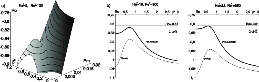
Figure 6: (a) The three-dimensional HMRI domain shows how the slices of it in the plane ${\rm Pm}=const$ converge smoothly to the inductionless HMRI domain for $\beta^{*}=0$. (b,c) HMRI domain ($m_{4}>0$) can exceed the inductionless bound $\rm Ro=2-2\sqrt{2}$ when $\rm Pm\neq 0$. Thin lines show the boundary of the inductionless HMRI domain, bold ones show that with $\rm Pm\neq 0$.

Despite the apparent discontinuities in the $(\beta^{*},\rm Ro)$-plane, the three-dimensional domain of HMRI in the $(\beta^{*},{\rm Pm},\rm Ro)$-space has a smooth boundary given by the expression $m_{4}=0$, Figure 6(a). As it is seen in Figure 6(a), the function ${\rm Ro}^{c}({\rm Pm},\beta^{*})$ has local extrema at some ${\rm Pm}\neq 0$, yielding regions of HMRI that are separated from each other in the plane $({\rm Pm},\beta^{*})$, Figure 5(b,c). Since the maximum is attained at small but finite values of $\rm Pm$, the corresponding boundary of HMRI in the $(\beta^{*},\rm Ro)$-plane at ${\rm Pm}\neq 0$ can exceed that in the inductionless limit (an instability induced by the viscosity $\omega_{\nu}\neq 0$) and, moreover, the limiting bound $\rm Ro=2-2\sqrt{2}$, as is clearly seen in Figure 6. The one-dimensional slices in the $(\beta^{*},\rm Ro)$-plane converge however to the region of the inductionless HMRI when $\rm Pm\rightarrow 0$. Therefore, in comparison to the inductionless limit, for ${\rm Pm}\neq 0$ we obtain higher values of the maximal Rossby numbers corresponding to the excitation of HMRI—a quite promising similarity of this local WKB analysis with the observation of HMRI for Keplerian flows with conducting boundaries in Rüdiger & Hollerbach (2007). In Figure 7, the evolution of the stability boundaries in the $({\rm Pm},{\rm Re}^{*})$-plane with the increase of $\beta^{*}$ demonstrates the details of the mechanism of reduction of the critical Reynolds number, which is another important characteristic of HMRI.

To clarify the nature of HMRI and SMRI and their relation to each other we inspect now the roots of the dispersion relation as functions of ${\rm Pm}$. Series expansions of the roots in the vicinity of ${\rm Pm}=0$ at $\beta^{*}=0$ yield

$$\lambda_{1,3} = \left[-1-{\rm Ha^{*}}^{2}\pm 2{\rm Re^{*}}\sqrt{-(1+{\rm Ro})}\right]\sqrt{\rm Pm}+o({\rm Pm^{1/2}}),$$

$$\lambda_{2,4} = -\frac{1}{\sqrt{\rm Pm}}+{\rm Ha^{*}}^{2}\sqrt{\rm Pm}+o({\rm Pm^{1/2}})$$ (70)

Therefore, two eigenvalues $\lambda_{1,3}$ branch from zero and the other two $\lambda_{2,4}$ branch from minus infinity. The eigenvalues $\lambda_{2,4}$ are real and negative, whereas the eigenvalues $\lambda_{1,3}$ are real in the vicinity of the origin for ${\rm Ro}\leq-1$ and complex otherwise with the frequency

$$\omega=2\Omega_{0}\frac{k_{z}}{k}\sqrt{{\rm Ro}+1}.$$

The eigenvalues $\lambda_{1,3}$ correspond to inertial waves with $\omega=\omega_{\rm C}:=2\Omega_{0}{k_{z}}/{k}$, if we assume rotation without shear $({\rm Ro}=0)$ and without damping, see e.g. Nornberg et al. (2009).

In the particular case, when $\beta^{*}=0$ and ${\rm Ro}=-1$ the dispersion equation is exactly solved

$$\lambda_{1,2} = \frac{-{\rm Pm}-1\pm\sqrt{({\rm Pm}-1)^{2}-4{\rm Pm}{\rm Ha^{*}}({\rm Ha^{*}}-2\sqrt{\rm Pm}){\rm Re^{*}}}}{2\sqrt{\rm Pm}},$$

$$\lambda_{3,4} = \frac{-{\rm Pm}-1\pm\sqrt{({\rm Pm}-1)^{2}-4{\rm Pm}{\rm Ha^{*}}({\rm Ha^{*}}+2\sqrt{\rm Pm}){\rm Re^{*}}}}{2\sqrt{\rm Pm}}.$$ (71)

The eigenvalues (4.3.1) are real near the origin, because ${\rm Ro}=-1$

$$\lambda_{1,3} = -\sqrt{\rm Pm}-{\rm Ha^{*}}^{2}\sqrt{\rm Pm}\pm 2{\rm Re^{*}}{\rm Ha^{*}}{\rm Pm}+o({\rm Pm}),$$

$$\lambda_{2,4} = -\frac{1}{\sqrt{\rm Pm}}+{\rm Ha^{*}}^{2}\sqrt{\rm Pm}\mp 2{\rm Re^{*}}{\rm Ha^{*}}{\rm Pm}+o(\rm Pm).$$ (72)

Equating the first of the equations (4.3.1) or (4.3.1) to zero we reproduce the expression for the threshold (69) at ${\rm Ro}=-1$.

In another particular case, when $\beta^{*}=0$, ${\rm Re^{*}}=0$, and ${\rm Ro}=0$ the exact solution to the dispersion equation is two double eigenvalues

$$\lambda=-\frac{1}{2}\left(\sqrt{\rm Pm}+\frac{1}{\sqrt{\rm Pm}}\right)\pm\sqrt{\frac{1}{4}\left(\sqrt{\rm Pm}-\frac{1}{\sqrt{\rm Pm}}\right)^{2}-{\rm Ha^{*}}^{2}}$$

that are expressed in terms of the viscous, resistive, and Alfvén frequencies in (30).

Consider the eigenvalues corresponding to the values of parameters of Figure 5. Since ${\rm Ro}=-0.85>-1$, there are two real and two complex branches of eigenvalues $\lambda=\lambda({\rm Pm})$ at $\beta^{*}=0$ , see Figure 8(a). One of the real branches that comes from minus infinity changes its sign at the threshold (69) and excites SMRI with zero eigenfrequency. Due to the large negative values of the real eigenvalues of the critical branch, there is no way to destabilize the flow at small $\rm Pm$. However, new opportunities for destabilization occur with the increase of $\beta^{*}$ that is accompanied by the qualitative change in the configuration of the eigenvalue branches.

When the azimuthal component of the magnetic field is switched on, the real eigenvalues of the critical branch get complex increments, Figure 8(b,c). With the increase of $\beta^{*}$, this critical real branch deforms and interacts with a stable complex one of an inertial wave until at $\beta^{*}\simeq 0.084$ they merge at a point with the origination of the double complex eigenvalue with the Jordan block known as an exceptional point or EP Berry (2004); Mailybaev et al. (2005), see Figure 8(b). Notice that another exceptional point corresponds to negative $\beta^{*}$. With the further increase of $\beta^{*}$ this configuration bifurcates into a new one, where parts of the stable and unstable branches are interchanged, Figure 8(c). The new critical eigenvalue branch consists of complex eigenvalues that demonstrate the typical generalized crossing scenario near an EP Or (1991); Keck et al. (2003), when real parts avoid crossing while imaginary ones cross and vice versa Figure 8(c).

In Figure 9 the ”surgery” of eigenvalue branches is clearly seen in the complex $({\rm Im}\lambda,{\rm Re}\lambda)$–plane. Although ”on the surface” (for ${\rm Re}(\lambda)>0$) nothing special happens, the deep reason for the exchange of the fragments between the branches is ”hidden” in the ${\rm Re}(\lambda)<0$ region at some finite value of $\rm Pm$ where an EP is formed, see Figure 9(c). The critical branch that was responsible for SMRI leaves its stable ”tail” coming from minus infinity (Figure 9(a,b)) and instead ”catches” a fragment of a stable branch of complex eigenvalues with small real parts that comes from zero (Figure 9(d-f)). This re-arranged branch of complex eigenvalues is much more prone to instabilities at low $\rm Pm$ than the original critical one as the further increase of $\beta^{*}$ confirms. Indeed, the negative real parts become smaller and around $\beta^{*}=0.7$ there appears a new interval of HMRI at those values of $\rm Pm$, at which SMRI did not exist, see Figure 10(a). This interval exactly corresponds to the island of HMRI shown in Figure 5(b,c). We note here that the numerical calculation of the roots of the dispersion relation confirms the boundaries of the regions of HMRI given by the Bilharz criterion: $m_{4}=0$.

The hidden exceptional point governs transfer of instability between the branch of (helically modified) SMRI and a complex branch of the inertial wave that after interaction becomes prone to destabilization. This qualitative effect explains why switching the azimuthal component of the magnetic field on we get HMRI as a travelling wave whereas SMRI was a stationary instability. Moreover, as Figure 10(c) shows, the new critical branch is characterized by a broad band of unstable frequencies while the tail of the branch responsible for SMRI corresponds to a more sharply selected unstable frequency which is close to zero at $\beta^{*}\neq 0$.

The above observations are in agreement with the observation of Liu et al. (2006) that, in contrast to SMRI, which is a destabilized slow Magneto-Coriolis wave, HMRI is a weakly destabilized inertial oscillation. Further results on interpretation of the HMRI as an unstable MHD-wave as well as on its relation to the dissipation-induced instabilities will be published elsewhere Fukumoto et al. .

4.3.2 Second scenario of HMRI excitation

The remarkable complexity of the phenomenon of HMRI manifests itself in different scenarios of destabilization. It turns out, that the transition from SMRI to HMRI through the exceptional point is not the only way to instabilities at low magnetic Prandtl numbers. At higher values of ${\rm Re}^{*}$ and ${\rm Ha}^{*}$, in the presence of the azimuthal magnetic field the inertial wave can become unstable without mixing with the critical SMRI branch.

In contrast to the scenario of the first type when one mixed complex branch becomes unstable at different intervals of ${\rm Pm}$ and causes both the essential HMRI and the helically modified SMRI, in the new situation the inertial wave causes the excitation of the essential HMRI and the critical real branch remains responsible for the helically modified SMRI, as is clearly seen in Figure 11.

Most surprisingly, the inertial wave branch can become unstable twice with the increase of $\beta^{*}$. The first time this happens in the vicinity of $\beta_{1}^{*}=\frac{1}{2}\sqrt{2}\simeq 0.707$, see Figure 11(b), then—in the neighborhood of $\beta_{2}^{*}=\frac{3}{2}\sqrt{2}\simeq 2.121$, as is visible in Figure 11(c). In the $({\rm Pm},\beta^{*})$-plane this yields two islands of the essential HMRI that coexist with the continent of the helically modified SMRI, Figure 12(a). The real parts of the unstable branches shown in black and grey in Figure 13 correspond to the first and second essential HMRI islands and to the continent of the helically modified SMRI, respectively.

The difference between the two HMRI scenarios is visible also in the other parameter planes. For example, in $({\rm Ha}^{*},\rm Ro)$-plane the domain of HMRI developed by the first scenario and corresponding to the HMRI-island of Figure 12(c) has an SMRI-like form with two peaks, see Figure 12(d). The second HMRI excitation scenario leads to the inclusions of the essential HMRI in the helically modified SMRI domain, Figure 12(b). Although the islands in Figure 12(a) and Figure 12(c) look similar, the former are slices of the two three-dimensional domains that intersect each other along an edge, while the latter are slices of the same smooth three-dimensional region of instability, cf. Figure 6(a).

5 Conclusions

The helical magnetorotational instability is a more complicated phenomenon than the standard one. We found evidences that HMRI can be identified with the destabilization of an inertial wave in contrast to SMRI that is a destabilized slow Magneto-Coriolis wave. We established two scenarios of transition from SMRI to HMRI: the first one is accompanied by the origination of a spectral exceptional point and a transfer of instability between modes while in the second scenario two independent eigenvalue branches become unstable. We distinguish between the essential HMRI that is characterized by small magnetic Prandtl numbers at which SMRI is not possible, smaller growth rates than SMRI, and by non-zero frequencies and the helically modified SMRI which is caused by a small perturbation of the unstable real eigenvalue branch and is thus characterized by high growth rates, small frequency and relatively high magnetic Prandtl numbers within the usual range of SMRI. With the use of the Bilharz stability criterion we established explicit expressions for the stability boundary and proved rigorously the bounds on the critical Rossby number for HMRI in the inductionless limit $(\rm Pm=0)$. Nevertheless, we revealed that for $\rm Pm\neq 0$ these bounds can be easily exceeded—an indicator in favor of the HMRI for small negative Rossby numbers. Finally, we found that for small negative Rossby numbers the essential HMRI forms separated islands that can coexist simultaneously in the $({\rm Pm},\beta^{*})$-plane.

Appendix A Linearization with respect to non-axisymmetric perturbations

We linearize equations (1)-(3) in the vicinity of the stationary solution (4)-(7) assuming general perturbations ${\bf u}={\bf u}_{0}+{\bf u}^{\prime}$, $p=p_{0}+p^{\prime}$, and ${\bf B}={\bf B}_{0}+{\bf B}^{\prime}$ and leaving only the terms of first order with respect to the primed quantities. With the notation Goodman & Ji (2002); Liu et al. (2006)

$$\partial_{t}=\frac{\partial}{\partial t},\quad\partial_{\phi}=\frac{\partial}{\partial\phi},\quad\partial_{R}=\frac{\partial}{\partial R},\quad\partial_{z}=\frac{\partial}{\partial z},\quad\partial_{R}^{\dagger}=\partial_{R}+\frac{1}{R},\quad D=\partial_{R}^{\dagger}\partial_{R}+\frac{1}{R^{2}}\partial^{2}_{\phi}+\partial_{z}^{2}$$ (A1)

we write the linearized equations in cylindrical coordinates, cf. Goodman & Ji (2002); Pessah & Psaltis (2005); Liu et al. (2006)

$$(\partial_{t}-\nu D)u_{R}^{\prime}-2\Omega u_{\phi}^{\prime}+\Omega\partial_{\phi}u_{R}^{\prime} = -\frac{1}{\rho}\left[\partial_{R}p^{\prime}+\frac{1}{\mu_{0}}\left(B_{z}^{0}{\partial_{R}}B_{z}^{\prime}+B_{\phi}^{0}{\partial_{R}}B_{\phi}^{\prime}-\frac{B_{\phi}^{0}}{R}B_{\phi}^{\prime}\right)\right]$$

$$+ \frac{1}{\mu_{0}\rho}\left(B_{z}^{0}{\partial_{z}}B_{R}^{\prime}+\frac{B_{\phi}^{0}}{R}\partial_{\phi}B_{R}^{\prime}-2\frac{B_{\phi}^{0}}{R}B_{\phi}^{\prime}\right)$$

$$- \nu\left(\frac{u_{R}^{\prime}}{R^{2}}+\frac{2}{R^{2}}{\partial_{\phi}u_{\phi}^{\prime}}\right),$$

$$({\partial_{t}}-\nu D)u_{\phi}^{\prime}+\frac{\kappa^{2}}{2\Omega}u_{R}^{\prime}+\Omega{\partial_{\phi}u_{\phi}^{\prime}} = -\frac{1}{\rho}\frac{1}{R}\left[{\partial_{\phi}p^{\prime}}+\frac{1}{\mu_{0}}\left(B_{z}^{0}{\partial_{\phi}B_{z}^{\prime}}+B_{\phi}^{0}{\partial_{\phi}B_{\phi}^{\prime}}\right)\right]$$

$$+ \frac{1}{\mu_{0}\rho}\left(B_{z}^{0}{\partial_{z}B_{\phi}^{\prime}}+\frac{B_{\phi}^{0}}{R}{\partial_{\phi}B_{\phi}^{\prime}}\right)+\nu\left(\frac{2}{R^{2}}{\partial_{\phi}u_{R}^{\prime}}-\frac{u_{\phi}^{\prime}}{R^{2}}\right),$$

$$({\partial_{t}}-\nu D)u_{z}^{\prime}+\Omega{\partial_{\phi}u_{z}^{\prime}} = -\frac{1}{\rho}\left[{\partial_{z}p^{\prime}}+\frac{1}{\mu_{0}}\left(B_{z}^{0}{\partial_{z}B_{z}^{\prime}}+B_{\phi}^{0}{\partial_{z}B_{\phi}^{\prime}}\right)\right]$$

$$+ \frac{1}{\mu_{0}\rho}\left(B_{z}^{0}{\partial_{z}B_{z}^{\prime}}+\frac{B_{\phi}^{0}}{R}{\partial_{\phi}B_{z}^{\prime}}\right),$$

$$({\partial_{t}}-\eta D)B_{R}^{\prime} = \frac{B_{\phi}^{0}}{R}{\partial_{\phi}u_{R}^{\prime}}-\Omega{\partial_{\phi}B_{\phi}^{\prime}}+B_{z}^{0}{\partial_{z}u_{R}^{\prime}}-\eta\left(\frac{B_{R}^{\prime}}{R^{2}}+\frac{2}{R^{2}}{\partial_{\phi}B_{\phi}^{\prime}}\right),$$

$$({\partial_{t}}-\eta D)B_{\phi}^{\prime} = B_{z}^{0}{\partial_{z}u_{\phi}^{\prime}}-B_{\phi}^{0}{\partial_{z}u_{z}^{\prime}}-B_{\phi}^{0}{\partial_{R}u_{R}^{\prime}}-u_{R}^{\prime}{\partial_{R}B_{\phi}^{0}}$$

$$+ u_{\phi}^{0}{\partial_{R}B_{R}^{\prime}}+u_{\phi}^{0}{\partial_{z}B_{z}^{\prime}}+B_{R}^{\prime}{\partial_{R}u_{\phi}^{0}}$$

$$+ \eta\left(\frac{2}{R^{2}}{\partial_{\phi}B_{R}^{\prime}}-\frac{B_{\phi}^{\prime}}{R^{2}}\right),$$

$$({\partial_{t}}-\eta D)B_{z}^{\prime} = -B_{z}^{0}{\partial_{R}u_{R}^{\prime}}-\frac{B_{z}^{0}}{R}u_{R}^{\prime}-\frac{B_{z}^{0}}{R}{\partial_{\phi}u_{\phi}^{\prime}}-\Omega{\partial_{\phi}B_{z}^{\prime}}+\frac{B_{\phi}^{0}}{R}{\partial_{\phi}u_{z}^{\prime}},$$

$$0 = \partial_{R}^{\dagger}u_{R}^{\prime}+\frac{1}{R}{\partial_{\phi}u_{\phi}^{\prime}}+{\partial_{z}u_{z}^{\prime}},$$

$$0 = \partial_{R}^{\dagger}B_{R}^{\prime}+\frac{1}{R}{\partial_{\phi}B_{\phi}^{\prime}}+{\partial_{z}B_{z}^{\prime}}.$$ (A2)

Figure 3: The domain according to equation (39) of SMRI (light grey, $\beta^{*}=0$) and that of HMRI (dark grey) for ${\rm Pm}=10^{-5}$ and ${\rm Re}^{*}=2\cdot 10^{5}$. The thin full line marks the stability boundary ${\rm Ro}={\rm Ro}^{c}$. The dashed, dotted, and bold lines bound the domains where the Bilharz minors $m_{1,2,3,4}>0$. The domain of HMRI which is adjacent to the intersection of these domains is shown in dark grey. The boundary to the HMRI domain (bold line) is $m_{4}=0$.

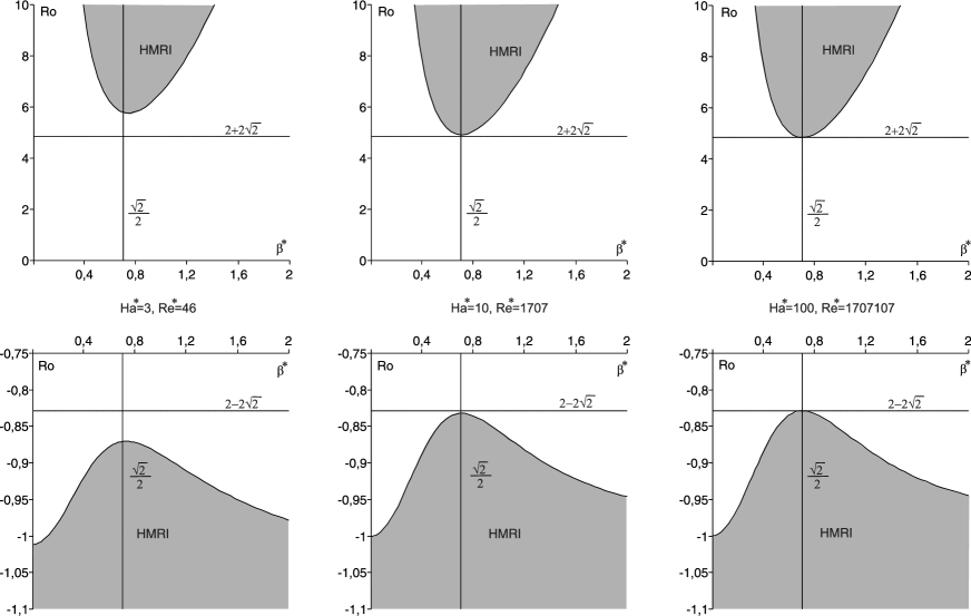
Figure 4: Inductionless approximation $(\rm Pm=0)$: Two domains (54) of HMRI (grey) are within the bounds (67). It is seen how the scaling law (68) works. HMRI is possible even for $\rm Pm=0$ – the paradox of inductionless magnetorotational instability Priede et al. (2007).

Figure 5: The relation of SMRI (right to the dashed line for $\beta^{*}=0$) and HMRI (grey area). For $\beta^{*}\neq 0$ a (semi)-island of HMRI exists in the neighborhood of $\beta^{*}=\sqrt{2}/2$ for the values of $\rm Pm$ at which SMRI was not possible in the absence of the azimuthal magnetic field $(\beta^{*}=0)$. The size of the HMRI island decreases with the increase of $\rm Ro$.

Figure 7: SMRI boundaries and those of HMRI in the plane (${\rm Pm},{\rm Re}^{*}$) for various values of $\rm Ro$. A considerable deformation of the boundaries when $\beta^{*}$ is switched on is seen in the region of small $\rm Pm$. The pictures are in agreement with the calculations of Rüdiger & Schultz (2008).

Figure 8: ${\rm Ha}^{*}=5$, ${\rm Re}^{*}=100$, ${\rm Ro}=-0.85$: Real and imaginary parts of eigenvalues $\lambda$ as functions of $\rm Pm$. (a) Two stable complex branches (inertial modes) and two real ones, one of the latter (grey) becomes positive and causes SMRI; (b) merging of the inertial mode with the deformed unstable SMRI-branch (grey) with the origination of an exceptional point (EP); (c) bifurcation yields new mixed eigenvalue branches that create new opportunities for instability at low $\rm Pm$.

Figure 9: ${\rm Ha}^{*}=5$, ${\rm Re}^{*}=100$, ${\rm Ro}=-0.85$: Eigenvalue trajectories in the complex plane when $\rm Pm$ changes from zero to ${\rm Pm}=0.011$ show the effect of transfer of instability between branches through a spectral exceptional point (EP). (a) SMRI is caused by the transition of a pure real eigenvalue from negative values to positive. (b) deformation of the critical branch (grey) for $\beta^{*}\neq 0$; (c) merging of the critical and stable branches with the origination of the double complex eigenvalue with the Jordan block - exceptional point (EP); (d-f) splitting of the EP and bifurcation of the eigenvalue trajectories: after a surgery the stable complex branch acquires an unstable tail of the critical branch (grey) and becomes unstable near the origin, which corresponds to an unstable traveling wave of HMRI.

Figure 10: ${\rm Ha}^{*}=5$, ${\rm Re}^{*}=100$, ${\rm Ro}=-0.85$, $\beta^{*}=0.7$: (a) Real part of the critical eigenvalue branch is positive while $\rm Pm$ is within the island or the continent of instability; (b) imaginary parts of stable and unstable branches; (c) trajectory of the critical eigenvalue that creates instability with the change of $\rm Pm$ from zero to ${\rm Pm}=0.011$.

Figure 11: ${\rm Ha}^{*}=17$, ${\rm Re}^{*}=28850$, ${\rm Ro}=-0.88$: (a) Stable inertial waves (black) and critical SMRI branch of real eigenvalues (grey) for $\beta^{*}=0$; (b) for $\beta^{*}=0.7$ one of the inertial wave branches becomes unstable independently of the SMRI branch; (c) for $\beta^{*}=2$ the same inertial wave branch becomes unstable a second time at higher frequencies independently of the SMRI branch.

Figure 12: (a) The first and second islands of the essential HMRI developed according to the second scenario in the neighborhood of $\beta^{*}=\sqrt{2}/2$ and $\beta^{*}=3\sqrt{2}/2$, (b) an essential HMRI inclusion in the helically modified SMRI domain, (c) an island of the essential HMRI developed according to the first scenario, (d) the corresponding view in the $({\rm Ha}^{*},{\rm Ro})$-plane.

Figure 13: ${\rm Ha}^{*}=17$, ${\rm Re}^{*}=28850$, ${\rm Ro}=-0.88$: (left, $\beta^{*}=0.7$) Real part of the first critical eigenvalue branch (grey) is positive when $\rm Pm$ is within the continent while for the second critical branch (black) it is within the first HMRI island; (right, $\beta^{*}=2$) real part of the first critical eigenvalue branch (grey) is positive when $\rm Pm$ is within the continent while for the second critical branch (black) it is within the second HMRI island.

References

- Balbus (2009) Balbus, S. A. 2009, Magnetorotational instability, Scholarpedia, 4(7), 2409.
- Balbus & Hawley (1991) Balbus, S. A. & Hawley, J. F. 1991, ApJ, 376, 214.
- Balbus & Henri (2008) Balbus, S. A. & Henri, P. 2008, ApJ 674, 408.
- Berry (2004) Berry, M.V. 2004, Czech. J. Phys. 54, 1039.
- Berry & Dennis (2003) Berry, M. V. & Dennis, M. R. 2003, Proc. R. Soc. Lond. A. 459, 1261.
- Bilharz (1944) Bilharz, H. 1944, Z. Angew. Math. Mech. 24, 77.
- Chandrasekhar (1960) Chandrasekhar, S. 1960, Proc. Natl. Acad. Sci., 46, 253.
- Dubrulle et al. (2005) Dubrulle, B., Marie, L., Normand, Ch., Richard, D., Hersant, F., & Zahn, J.-P. 2005, Astron. Astrophys. 429, 1.
- (9) Fukumoto, Y., Kirillov, O. N., & Stefani, F. (in preparation)
- Goodman & Ji (2002) Goodman, J. & Ji, H. 2002, J. Fluid Mech., 462, 365.
- Hollerbach & Rüdiger (2005) Hollerbach, R., & Rüdiger, G. 2005, Phys. Rev. Lett. 95, 124501.
- Hollerbach et al. (2009) Hollerbach, R., Teeluck, V. & Rüdiger, G. 2009, Phys. Rev. Lett., submitted (arXiv:0910.0206)
- Ji et al. (2001) Ji, H., Goodman, G., & Kageyama, J. A. 2001, MNRAS, 325, L1.
- Ji et al. (2006) Ji, H. T., Burin, M, Schartman, E. & Goodman, J. 2006, Nature, 444, 343
- Keck et al. (2003) Keck, F., Korsch, H.-J., & Mossmann, S. 2003, J. Phys. A: Math. Gen. 36, 2125.
- Kirillov et al. (2005) Kirillov, O. N., Mailybaev, A. A., & Seyranian, A. P. 2005, J. Phys. A: Math. Gen., 38(24), 5531.
- Kirillov (2007) Kirillov, O. N. 2007, Int. J. of Non-Lin. Mech. 42(1), 71.
- Kirillov (2009) Kirillov, O. N. 2009, Proc. R. Soc. A, 465, 2703.
- Kirillov (2010) Kirillov, O. N. 2010, Z. Angew. Math. Phys. 61(2), doi 10.1007/s00033-009-0032-0
- Knobloch (1992) Knobloch, E. 1992, MNRAS, 255, P25.
- Knobloch (1996) Knobloch, E. 2001, Phys. Fluids 8, 1446.
- Krechetnikov & Marsden (2007) Krechetnikov, R. & Marsden, J. E. 2007, Rev. Mod. Phys. 79, 519.
- Lakhin & Velikhov (2007) Lakhin, V. P. & Velikhov, E. P. 2007, Phys. Lett. A, 369, 98.
- Lehnert (1954) Lehnert, B. 1954, Astrophysical Journal, 119, 647.
- Lienard & Chipart (1914) Lienard, A. & Chipart, H. 1914, J. Math. Pures Appl. 10, 291.
- Liu et al. (2006) Liu, W., Goodman, J., Herron, I., & Ji, H. 2006, Phys. Rev. E., 74, 056302.
- Liu et al. (2007) Liu, W., Goodman, J., & Ji, H. 2007, Phys. Rev E, 76, 016310.
- Liu (2008) Liu, W. 2008, ApJ, 684, 515.
- Liu (2009) Liu, W. 2009, ApJ, 692, 998.
- Mailybaev et al. (2005) Mailybaev, A.A., Kirillov, O.N., Seyranian, A.P. 2005, Phys. Rev. A 72, 014104
- Marden (1966) Marden, M. 1966, Geometry of polynomials. Second edition. Mathematical Surveys, No. 3 American Mathematical Society, Providence, R.I. xiii+243 pp.
- Noguchi et al. (2002) Noguchi, K., Pariev, V. I., Colgate, S. A., Beckley, H. F., & Nordhaus, J. 2002, ApJ, 575, 1151.
- Nornberg (2008) Nornberg, M. 2008, Bull. Amer. Phys. Soc., 53(14), GI2.00003.
- Nornberg et al. (2009) Nornberg, M.D., Ji, H., Schartman, E., Roach, A., & Goodman, J. 2009, Observation of magnetocoriolis waves in a liquid metal Taylor-Couette experiment, PPPL-4448, 14 p.
- Or (1991) Or, A. C. 1991, Quart. J. Mech. Appl. Math. 44(4), 559.
- Pessah & Psaltis (2005) Pessah, M. E. & Psaltis, D. 2005, ApJ, 628, 879.
- Priede et al. (2007) Priede, J., Grants, I. & Gerbeth, G. 2007, Phys. Rev. E, 75, 047303.
- Priede & Gerbeth (2009) Priede, J. & Gerbeth, G. 2009, Phys. Rev. E, 79, 046310.
- Roberts & Loper (1979) Roberts, P. H. & Loper, D. E. 1979, J. Fluid Mech. 90, 641.
- Rosner et al. (2004) Rosner, R., Rüdiger, G., & Bonanno, A., eds. 2004, AIP Conf. Proc. 733, MHD Couette flows: Experiments and Models (New York: AIP)
- Rüdiger et al. (2005) Rüdiger, G., Hollerbach, R., Schultz, M., & Shalybkov, D. A. 2005, Astron. Nachr. 326, 409.
- Rüdiger et al. (2006) Rüdiger, G., Hollerbach, R., Stefani, F., Gundrum, Th., Gerbeth, G., & Rosner, R. 2006, AJ, 649, L145.
- Rüdiger & Hollerbach (2007) Rüdiger, G. & Hollerbach, R. 2007, Phys. Rev. E., 76, 068301.
- Rüdiger & Schultz (2008) Rüdiger, G. & Schultz, M. 2008, Astron. Nachr., 329, 659.
- Rüdiger et al. (2008) Rüdiger, G., Hollerbach, R., Schultz, M., & Shalybkov, D. A. 2008, Astron. Nachr. 329, 659.
- Sisan et al. (2004) Sisan, D. R., Mujica, N., Tillotson, W. A., Huang, Y. M. Dorland, W., Hassam, A. B., Antonsen, T. M., & Lathrop, D. P. 2004, Phys. Rev. Lett. 93, 114502.
- Stefani et al. (2006) Stefani, F., Gundrum, Th., Gerbeth, G., Rüdiger, G., Schultz, M., Szklarski, J., & Hollerbach, R. 2006, Phys. Rev. Lett., 97, 184502.
- Stefani et al. (2007) Stefani, F., Gundrum, Th., Gerbeth, G., Rüdiger, G., Szklarski, J., & Hollerbach, R. 2007, New J. Phys., 9, 295.
- (49) Stefani, F., Gailitis, A., & Gerbeth, G. 2008, Z. Angew. Math. Mech., 88, 930.
- (50) Stefani, F., Gerbeth, G., Gundrum, Th., Szklarski, J., Rüdiger, G., Hollerbach R. 2008, Astron. Nachr. 329, 652.
- (51) Stefani, F., Gerbeth, G., Gundrum, Th., Szklarski, J., Rüdiger, G., & Hollerbach, R. 2009, Magnetohydrodynamics, 45, 135.
- (52) Stefani, F., Gerbeth, G., Gundrum, T., Hollerbach, R., Priede, J., Rüdiger, G., & Szklarski, J. 2009, Phys. Rev. E, in press, arXiv:0904.1027
- Szklarski (2007) Szklarski, J. 2007, Astron. Nachr., 328, 499.
- Tayler (1973) Tayler, R. J. 1973, MNRAS, 161, 365.
- Umurhan (2006) Umurhan, O. M. 2006, MNRAS, 365, 85.
- Velikhov (1959) Velikhov, E. P. 1959, Sov. Phys. JETP, 36, 995.
- Wendl (1999) Wendl, M. C. 1999, Phys. Rev. E 60, 6192.