A posteriori error analysis for finite element solution of elliptic differential equations using equidistributing meshes

Abstract

The paper is concerned with the adaptive finite element solution of linear elliptic differential equations using equidistributing meshes. A strategy is developed for defining this type of mesh based on residual-based a posteriori error estimates and rigorously analyzing the convergence of a linear finite element approximation using them. The existence and computation of equidistributing meshes and the continuous dependence of the finite element approximation on mesh are also studied. Numerical results are given to verify the theoretical findings.

AMS 2000 Mathematics Subject Classification. 65M50,65M60, 65L50, 65L60

Key Words. Mesh adaptation, equidistribution, error analysis, finite element method

Abbreviated title. Error analysis for equidistributing meshes

1 Introduction

We are concerned with the convergence of the linear finite element solution of elliptic differential equations using equidistributing meshes. An equidistributing mesh of $N$ elements for $\Omega\equiv(0,1)$ is a mesh $x_{0}=0<x_{1}<\cdots<x_{N}=1$ satisfying the so-called equidistribution principle [12, 19]

$$\int_{x_{i-1}}^{x_{i}}\rho(x)dx=\frac{1}{N}\int_{0}^{1}\rho(x)dx,\quad i=1,...,N$$ (1)

where $\rho=\rho(x)$ is a user-prescribed, strictly positive function. Function $\rho(x)$, referred to as an adaptation function, can be interpreted as an “error” density function, with $\int_{0}^{1}\rho(x)dx$ being the total “error”. Equation (1) implies that $\rho(x)$ is evenly distributed among the mesh elements.

Equidistributing meshes are known to produce optimal error bounds and have been widely used for adaptive numerical solution of differential equations. Their theoretical studies have also attracted considerable attention from researchers; e.g., see [12, 19, 20, 22, 30, 38] on best approximations with variable nodes, [39, 40, 41] on regression problems in statistics, [2, 34, 44] on adaptive numerical solution of differential equations, and [6, 7, 8, 16, 25, 26, 27, 28, 29, 36, 37] for more recent works. A focus of these studies has been on error analysis, i.e., to understand how accurate an approximation or a numerical solution can be on an equidistributing mesh. Unfortunately, this has proven to be a difficult task due to the highly nonlinear coupling between the mesh and the solution. The analysis can be significantly simplified by taking a priori meshes defined using the exact solution or some information of the exact solution. Interestingly, almost all of the existing analyses have been done in this way. For example, Pereyra and Sewell [34] choose a mesh to equidistribute a form of the truncation error and obtain an asymptotical bound for it for the finite difference solution of two-point boundary value problems. Qiu et al. [36, 37] and Beckett and Mackenzie [6, 7, 8, 29] investigate the uniform convergence of finite difference and finite element approximations for singularly perturbed problems for meshes determined using the equidistribution principle and the singular part of the exact solution. Chen and Xu [17] show that a standard finite element method and a new streamline diffusion finite element method produce stable and accurate approximations for a singularly perturbed convection-diffusion problem provided that the mesh properly adapts to the singularity of the solution. Huang et al. [25, 26, 27] and Chen et al. [16] study multi-dimensional interpolation problems using equidistributing meshes which depend on the function under consideration.

The noticeable exceptions are the work [2] and [28] where a posteriori equidistributing meshes, or equidistributing meshes determined by the computed solution, are considered. More specifically, Babus̆ka and Rheinboldt [2] consider the linear finite element solution of a one-dimensional elliptic problem and develop a functional from a residual-based a posteriori error estimate in lieu of asymptotic approximation and coordinate transformation. Using the optimal coordinate transformation obtained by minimizing the functional, Babus̆ka and Rheinboldt show that a mesh is asymptotically optimal if the residual-based error estimate is evenly distributed among the mesh elements. Kopteva and Stynes [28] study an upwind finite difference discretization of one-dimensional quasi-linear convection-diffusion problems without turning points and develop a convergence analysis for the discretization where the mesh is determined by the computed solution through the equidistribution principle and the arc-length adaptation function.

In this paper we are concerned with convergence analysis for the finite element solution using a posteriori equidistributing meshes. The goal is to develop a systematic approach for defining these meshes such that both their error analysis and computation can be done in an a posteriori manner. At the same time we would like the approach to be general enough so that it can apply to any standard finite element method and have no essential limitations for multi-dimensional generalizations. Furthermore, the approach should be mathematically rigorous. Particularly, it should not rely on asymptotic approximation or continuous coordinate transformations as in [2, 27]. Several other issues, such as the existence and computation of equidistributing meshes and the continuous dependence of the linear finite element solution on mesh, are also studied in the paper. The main results are given in §2.

Since Dörfler’s seminal work [21] significant progress has been made on the convergence analysis of adaptive finite element methods based on a posteriori error estimates; e.g. see [9, 13, 14, 15, 31, 32, 42]. It should, however, be pointed out that there are essential differences between those works and the current one. The former ones are dealt with adaptive mesh refinement using specially designed marking strategies and their convergence results are typically measured in terms of refinement levels, whereas the current work is concerned with equidistributing meshes (including their existence, generation, optimality, and error analysis) and our results are measured in terms of the number of mesh elements (cf. Theorems 2.1 and 2.2). It does not seem that the existing convergence analysis for mesh refinement can apply directly to equidistributing meshes and neither can the current results be covered by the existing ones. On the other hand, adaptive mesh refinement and equidistribution do share some common ground. For example, an equidistributing mesh can be generated through mesh refinement (e.g., see [10, 26]) (and other strategies (e.g. see [24] for a variational approach)), and the concept of mesh equidistribution is often used in mesh refinement algorithms and computer codes for maximizing the efficiency of computation (e.g., see [33]). Relations between convergence results for adaptive mesh refinement and equidistribution may thus deserve further investigations.

The paper is organized as follows. The description of the mathematical problem and the main results are given in §2. The approach for defining equidistributing meshes and analyzing the corresponding finite element error is developed in §3. An iterative algorithm for computing the meshes is proposed and numerical results are presented in §4. The continuous dependence of the finite element solution on mesh and the existence of equidistributing meshes are studied in §5 and §6, respectively.

2 Main results

We consider the boundary value problem of a linear elliptic differential equation

$$-(au^{\prime})^{\prime}+bu^{\prime}+cu=f,\qquad\mbox{ in }\Omega$$ (2)

$$u(0)=u(1)=0,$$ (3)

where $a(x)$, $b(x)$, $c(x)$, and $f(x)$ are given functions satisfying

$$\quad a,b\in W^{1,\infty}(\Omega),\quad c\in L^{\infty}(\Omega),\quad f\in L^{2}(\Omega),$$ (4)

and

$$a(x)\geq a_{0}>0,\quad c(x)-\frac{1}{2}b^{\prime}(x)\geq 0,\quad a.e.\mbox{ in }\Omega$$ (5)

for some constant $a_{0}$. Here, $W^{1,\infty}(\Omega)$ denotes the Sobolev space of functions whose derivatives are in $L^{\infty}(\Omega)$. The variational form of problem (2) and (3) is to find $u\in V\equiv H^{1}_{0}(\Omega)$ such that

$$B(u,v)=(f,v),\quad\forall v\in V$$ (6)

where

$$B(u,v)=\int_{\Omega}(au^{\prime}v^{\prime}+bu^{\prime}v+cuv)dx,\quad(f,v)=\int_{\Omega}fvdx.$$ (7)

For a given mesh

$$\pi_{h}:\quad x_{0}=0<x_{1}<\cdots<x_{N}=1$$ (8)

with $h=\max_{i}(x_{i}-x_{i-1})$, a linear finite element approximation to the solution of (6) is defined as $u_{h}\in V_{h}$ satisfying

$$B(u_{h},v_{h})=(f,v_{h}),\quad\forall v_{h}\in V_{h}$$ (9)

where the linear finite element space $V_{h}$ is given by

$$V_{h}=\mbox{span}\{\phi_{1},...,\phi_{N-1}\},$$ (10)

with $\phi_{i}$’s being linear basis functions associated with mesh points $x_{i}$’s.

We are concerned with adaptive finite element solution of (2) and (3) using equidistributing meshes. For this purpose, we choose the mesh according to the equidistribution principle (1) or

$$\rho_{i}h_{i}=\int_{x_{i-1}}^{x_{i}}\rho(x)dx=\frac{\sigma_{h}}{N},\quad i=1,...,N$$ (11)

where

$$h_{i}=x_{i}-x_{i-1},$$ (12)

$$\sigma_{h}=\sum_{i}\rho_{i}h_{i},$$ (13)

$$\left.\rho\right|_{(x_{i-1},x_{i})}=\rho_{i}\equiv\left(1+\frac{1}{\alpha_{h}}\left<r_{h}\right>_{i}^{2}\right)^{\frac{1}{3}},\quad i=1,...,N$$ (14)

$$\alpha_{h}=\left[\sum_{i}h_{i}\left<r_{h}\right>_{i}^{\frac{2}{3}}\right]^{3},$$ (15)

$$r_{h}=f+a^{\prime}u_{h}^{\prime}-bu_{h}^{\prime}-cu_{h},$$ (16)

$$\left<r_{h}\right>_{i}=\left(\frac{1}{h_{i}}\int^{x_{i}}_{x_{i-1}}|r_{h}|^{2}dx\right)^{\frac{1}{2}}.$$ (17)

Here, $u_{h}$ is the solution of (9), $r_{h}$ is the residual function, $\rho(x)$ is the piecewise constant adaptation function, and $\left<r_{h}\right>_{i}$ is the $L^{2}$ average of $r_{h}$ over $(x_{i-1},x_{i})$.

The choice (14) for the adaptation function is based on an a posteriori error estimate for the linear finite element solution; see §3. Clearly, the choice depends on the computed solution and thus the mesh is a posteriori. Unfortunately, this also means that the mesh and the computed solution are coupled with each other. The system for $u_{h}$ and $\pi_{h}$ consists of algebraic equations (9) and (11) and the boundary conditions $x_{0}=0$ and $x_{N}=1$ and is typically solved iteratively; see Fig. 1. An algorithm of this type is given in §4. The existence of the equidistributing mesh is stated in Theorem 2.4 below.

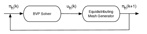
Figure 1: Illustration of the iterative solution procedure for the finite element solution using equidistributing meshes.

Notation. The $L^{2}$-norm on $\Omega$ is denoted by $\|\cdot\|_{\Omega}$ and other $L^{p}$-norm by $\|\cdot\|_{L^{p}(\Omega)}$, with the latter being extended to the situation $0<p<1$. Let

$$\bar{v}=\|v\|_{L^{\infty}(\Omega)},\quad\forall v\in L^{\infty}(\Omega).$$ (18)

We use $C$ as a generic constant which may have different values at different appearances. In most part of this paper, constants are considered as numbers that may depend on the domain and coefficients $a(x)$, $b(x)$, and $c(x)$ of differential equation (2) but not on the solution $u$, the right-hand sider $f$, and the mesh employed in the finite element solution. The exceptions are Theorems 2.3 and 2.4 and §5 and §6 where constants may further depend on $u$ and $f$.

Define

$$\rho_{0}=\left[1+\gamma\left(\frac{\|r\|_{L^{\infty}(\Omega)}}{\|r\|_{L^{\frac{2}{3}}(\Omega)}}\right)^{\frac{2}{3}}\right]^{2},$$ (19)

where $\gamma$ is a positive constant dependent on the domain and coefficients of equation (2). The definition of $\gamma$ is given in the proof of Lemma 6.1. The same lemma also shows that $\rho_{0}$ is the upper bound on the adaptation function defined in (14).

From (8), the mesh $\pi_{h}$ corresponds one-to-one to the $(N-1)$-component vector $X=(x_{1},...,x_{N-1})^{\top}$. For this reason, occasionally $X$ is directly referred to as a mesh. Let

$$S_{N}= \left\{\frac{}{}\right.X\in\Re^{N-1}:\;x_{0}=0<x_{1}<\cdots<x_{N-1}<x_{N}=1,$$ (20)

$$\quad\left.\frac{1}{\rho_{0}N}\leq h_{i}\leq\frac{2}{N},\;\;i=1,...,N\;\right\}.$$

It is easy to verify that $S_{N}$ is a closed, convex subset of $\Re^{N-1}$. The set is equipped with the maximum norm, viz.,

$$\|X\|_{\infty}=\max_{i}|x_{i}|,\quad\forall X\in S_{N}.$$ (21)

This set plays an important role in the study of the existence of equidistributing meshes and the continuous dependence of the finite element solution on mesh. Any $N$-cell equidistributing mesh is a member of this set.

The main results of this paper are summarized in the following four theorems.

      Theorem 2.1

(Convergence for equidistributing meshes) Define $\rho$ and $\alpha_{h}$ as in (14) and (15), respectively. For any equidistributing mesh satisfying (11), the error for the linear finite element solution (9) is bounded by

$$\|(u-u_{h})^{\prime}\|_{\Omega}\leq\frac{C\sqrt{\alpha_{h}}}{N},$$ (22)

where $\alpha_{h}$ has the property

$$\lim_{N\to\infty}\sqrt{\alpha_{h}}=\|r\|_{L^{\frac{2}{3}}(\Omega)}$$ (23)

and $r$ is the continuous “residual” function $r$ defined as

$$r=f+a^{\prime}u^{\prime}-bu^{\prime}-cu.$$ (24)

If further $r$ satisfies $r^{\prime}\in L^{1}(\Omega)$, then there exists a positive constant $c$ such that for $N>c$,

$$\left(1+\left(\frac{c}{N}\right)^{\frac{2}{3}}\right)^{-\frac{3}{2}}\|r\|_{L^{\frac{2}{3}}(\Omega)}\leq\sqrt{\alpha_{h}}\leq\left(1-\left(\frac{c}{N}\right)^{\frac{2}{3}}\right)^{-\frac{3}{2}}\left[\|r\|_{L^{\frac{2}{3}}(\Omega)}^{\frac{2}{3}}+\left(\frac{c\|r^{\prime}\|_{L^{1}(\Omega)}}{N}\right)^{\frac{2}{3}}\right]^{\frac{3}{2}}.$$ (25)

The proof of this theorem is given in §3.4. The theorem shows that the error has the asymptotic bound as

$$\lim_{N\to\infty}N\;\|(u-u_{h})^{\prime}\|_{\Omega}\leq C\|r\|_{L^{\frac{2}{3}}(\Omega)}.$$ (26)

This is compared with the error bound for a uniform mesh (cf. Lemma 3.3)

$$\|(u-u_{h})^{\prime}\|_{\Omega}\leq\frac{C_{1}\|r\|_{\Omega}}{N}.$$ (27)

Since

$$\|r\|_{L^{\frac{2}{3}}(\Omega)}\leq\|r\|_{\Omega}$$

and particularly, the left-hand side is much smaller than the right-hand side when $r$ ($\sim au^{\prime\prime}$) is non-smooth, the theorem implies that the error bound for an equidistributing mesh can be much smaller than that for a uniform mesh. This explains why an adaptive mesh often produces a more accurate solution than a uniform one when the solution is non-smooth.

In practice, it is more realistic to use a quasi-equidistributing mesh than an exact one. A quasi-equidistributing mesh is a mesh satisfying

$$\frac{N\rho_{i}h_{i}}{\sigma_{h}}\leq\kappa\qquad i=1,...,N$$ (28)

for some positive constant $\kappa$ independent of $i$ and $N$. The following theorem, proved in §3.4, shows that for small $\kappa$, a quasi-equidistributing mesh leads to a comparable error bound as an exact equidistributing mesh.

      Theorem 2.2

(Convergence for quasi-equidistributing meshes) Define $\rho$ and $\alpha_{h}$ as in (14) and (15), respectively. Then for any quasi-equidistributing mesh satisfying (28), the error for the linear finite element solution (9) is bounded by

$$\|(u-u_{h})^{\prime}\|_{\Omega}\leq\frac{C\sqrt{\alpha_{h}\kappa^{3}}}{N},$$ (29)

where $\alpha_{h}$ satisfies (23).

If further $r$ satisfies $r^{\prime}\in L^{1}(\Omega)$, then there exists a positive constant $c$ such that for $N>\kappa c$,

$$\left(1+\left(\frac{\kappa c}{N}\right)^{\frac{2}{3}}\right)^{-\frac{3}{2}}\|r\|_{L^{\frac{2}{3}}(\Omega)}\leq\sqrt{\alpha_{h}}\leq\left(1-\left(\frac{\kappa c}{N}\right)^{\frac{2}{3}}\right)^{-\frac{3}{2}}\left[\|r\|_{L^{\frac{2}{3}}(\Omega)}^{\frac{2}{3}}+\left(\frac{\kappa c\|r^{\prime}\|_{L^{1}(\Omega)}}{N}\right)^{\frac{2}{3}}\right]^{\frac{3}{2}},$$ (30)

where $r$ is defined in (24).

      Theorem 2.3

(Continuous dependence of finite element solution on mesh) Assume that $f\in L^{\infty}(\Omega)$ and $u\in H^{2}(\Omega)$. Then for any meshes $X,\;\tilde{X}\in S_{N}$ satisfying

$$\|X-\tilde{X}\|_{\infty}<\frac{1}{\rho_{0}N},$$ (31)

the corresponding linear finite element solutions, $u_{h}$ and $u_{\tilde{h}}$, satisfy

$$\|(u_{h}-u_{\tilde{h}})^{\prime}\|_{L^{1}(\Omega)} \leq CN\|X-\tilde{X}\|_{\infty},$$ (32)

$$\|u_{h}-u_{\tilde{h}}\|_{\Omega} \leq CN^{-\frac{1}{2}}\|X-\tilde{X}\|^{\frac{1}{2}}_{\infty},$$ (33)

$$\left|\|u_{h}\|_{E}^{2}-\|u_{\tilde{h}}\|_{E}^{2}\right| \leq CN^{-\frac{1}{2}}\|X-\tilde{X}\|^{\frac{1}{2}}_{\infty},$$ (34)

where $\|\cdot\|_{E}$ denotes the energy norm associated with the bilinear form $B(\cdot,\cdot)$, viz.,

$$\|v\|_{E}^{2}=\int_{\Omega}\left(av^{\prime 2}+(c-\frac{1}{2}b^{\prime})v^{2}\right)dx.$$

      Theorem 2.4

(Existence of equidistributing meshes) Assume that $f\in L^{\infty}(\Omega)$ and $u\in H^{2}(\Omega)$. For sufficiently large $N$ (i.e., $N\geq N_{0}$ where $N_{0}$ is defined in Lemma 6.1), there exists at least an equidistributing mesh satisfying (11).

The above two theorems are proven in §5 and §6, respectively. An iterative algorithm for computing equidistributing meshes is proposed in §4. The numerical results presented in §4 demonstrate that the algorithm converges for sufficiently large $N$ and faster for larger $N$. This is consistent with what observed by Pryce [35] and Xu et al. [45] on the convergence of de Boor’s algorithm for generating equidistributing meshes for given adaptation functions.

3 Error analysis for finite element solution using equidistributing meshes

In this section we present an error analysis for equidistributing meshes satisfying (11) and quasi-equidistributing meshes satisfying (28). The approach we use consists of three major steps, deriving a residual-based a posteriori error estimate, defining the adaptation function (14) based on the estimate, and developing the error analysis for the corresponding equidistributing mesh. This approach shares some similarity with that used in [25, 26, 27] for analyzing interpolation error in multi-dimensions. The main difference lies in that the current analysis is based on an a posteriori error estimate and is mathematically rigorous, whereas the analysis in [25, 26, 27] is based on interpolation error bounds (depending on the exact solution) and valid only in an asymptotic sense.

3.1 Preliminary results

For completeness and for easy reference we list here some preliminary results without giving their proofs. These results can be found in most finite element textbooks, e.g. [11, 18].

      Lemma 3.1

The bilinear form $B(\cdot,\cdot)$ defined in (7) has the properties

$$a_{0}\,\|v^{\prime}\|_{\Omega}^{2}\leq B(v,v)\leq C\|v^{\prime}\|_{\Omega}^{2},\qquad\forall v\in V$$ (35)

$$B(u,v)\leq C\|u^{\prime}\|_{\Omega}\,\|v^{\prime}\|_{\Omega},\qquad\forall u,v\in V.$$ (36)

Moreover, the solution of the problem (6) satisfies

$$\|u^{\prime}\|_{\Omega}\leq C\|f\|_{\Omega}.$$ (37)

      Lemma 3.2

Given a mesh $\pi_{h}$, denote by $\Pi_{h}$ the operator for piecewise linear interpolation, i.e.,

$$\Pi_{h}v(x)=\sum_{i=0}^{N}v(x_{i})\phi_{i}(x),\qquad\forall v\in H^{1}(\Omega)$$ (38)

where $\phi_{i}$’s are the linear basis functions associated with mesh points $x_{i}$’s. Then, for any $K_{i}=(x_{i-1},x_{i})$,

$$\|v-\Pi_{h}v\|_{K_{i}} \leq Ch_{i}\|(v-\Pi_{h}v)^{\prime}\|_{K_{i}},\qquad\forall v\in H^{1}(K_{i})$$ (39)

$$\|(v-\Pi_{h}v)^{\prime}\|_{K_{i}} \leq Ch_{i}\|v^{\prime\prime}\|_{K_{i}},\qquad\forall v\in H^{2}(K_{i})$$ (40)

$$\|(v-\Pi_{h}v)^{\prime}\|_{K_{i}} \leq C\|v^{\prime}\|_{K_{i}},\qquad\forall v\in H^{1}(K_{i}).$$ (41)

The error for the finite element solution $u_{h}$, $e_{h}=u-u_{h}$, satisfies the orthogonality property and the error equation, viz.,

$$B(e_{h},v_{h})=0,\qquad\forall v_{h}\in V_{h}$$ (42)

$$B(e_{h},v)=(f,v)-B(u_{h},v),\qquad\forall v\in V.$$ (43)

      Lemma 3.3

The finite element solution $u_{h}$ defined in (9) satisfies

$$\|u_{h}^{\prime}\|_{\Omega}\leq C\|f\|_{\Omega}.$$ (44)

Moreover, if the solution of the continuous problem (6) satisfies $u\in H^{2}(\Omega)$ and the mesh has the property

$$h\equiv\max_{i}h_{i}\leq\frac{C_{1}}{N}$$ (45)

for some positive constant $C_{1}$, the error is bounded by

$$\|(u-u_{h})^{\prime}\|_{\Omega}\leq\frac{C\|r\|_{\Omega}}{N}.$$ (46)

Obviously, a uniform mesh satisfies the condition (45). The finite element error for a uniform mesh can thus be bounded as in (46).

3.2 An a posteriori error estimate

We now derive a residual-based a posteriori error estimate for the finite element solution. The general procedure for this type of error estimation can be seen, e.g., in [1, 3, 4, 5, 43].

      Lemma 3.4

The error $e_{h}=u-u_{h}$ is bounded by

$$\|(u-u_{h})^{\prime}\|_{\Omega}^{2}\leq C\eta_{h}^{2}=C\sum_{i}h_{i}^{2}\|r_{h}\|_{K_{i}}^{2},$$ (47)

where $r_{h}$ is defined in (16), i.e., $r_{h}=f+a^{\prime}u_{h}^{\prime}-bu_{h}^{\prime}-cu_{h}$.

Proof. Using orthogonality property (9), error equation (42), integration by parts, Lemma 3.2, and Schwarz’ inequality, we have, for any $v\in V$,

$$B(e_{h},v) = B(e_{h},v-\Pi_{h}v)$$

$$= (f,v-\Pi_{h}v)-B(u_{h},v-\Pi_{h}v)$$

$$= \sum_{i}\int_{K_{i}}r_{h}(v-\Pi_{h}v)dx$$

$$\leq \sum_{i}\|r_{h}\|_{K_{i}}\|v-\Pi_{h}v\|_{K_{i}}$$

$$\leq C\sum_{i}\|r_{h}\|_{K_{i}}\cdot h_{i}\|v^{\prime}\|_{K_{i}}$$

$$\leq C\left(\sum_{i}h_{i}^{2}\|r_{h}\|_{K_{i}}^{2}\right)^{1/2}\|v^{\prime}\|_{\Omega}.$$

Then (47) follows by taking $v=e_{h}$ in the above inequality and using Lemma 3.1.

3.3 Determination of optimal adaptation function

Up to this point the mesh has been assumed to be arbitrary and Lemma 3.4 has been obtained for this general mesh. From now on we shall focus on equidistributing meshes determined according to the a posteriori error estimate (47).

As we can see from (1), the key for the determination of equidistributing meshes is to define an appropriate adaptation function $\rho=\rho(x)>0$. To this end, we regularize $\eta_{h}$ in (47) with a positive constant $\alpha_{h}>0$ (to be determined), i.e.,

$$\eta_{h}^{2} = \sum_{i}h_{i}^{2}\|r_{h}\|_{K_{i}}^{2}$$ (48)

$$\leq \sum_{i}h_{i}^{3}\left(\alpha_{h}+\left<r_{h}\right>_{i}^{2}\right)$$

$$= \alpha_{h}\sum_{i}h_{i}^{3}\left(1+\frac{1}{\alpha_{h}}\left<r_{h}\right>_{i}^{2}\right)\equiv\tilde{\eta}_{h}^{2}.$$

Notice that $\tilde{\eta}_{h}\to\eta_{h}$ as $\alpha_{h}\to 0$. Moreover,

$$\tilde{\eta}_{h}^{2} = \alpha_{h}\sum_{i}\left[h_{i}\left(1+\frac{1}{\alpha_{h}}\left<r_{h}\right>_{i}^{2}\right)^{\frac{1}{3}}\right]^{3}$$ (49)

$$\geq \frac{\alpha_{h}}{N^{2}}\left[\sum_{i}h_{i}\left(1+\frac{1}{\alpha_{h}}\left<r_{h}\right>_{i}^{2}\right)^{\frac{1}{3}}\right]^{3}.$$

It is easy to see that the equality in the above inequality holds for any equidistributing mesh when the adaptation function $\rho(x)$ is chosen as in (14), i.e.,

$$\left.\rho\right|_{K_{i}}=\rho_{i}\equiv\left(1+\frac{1}{\alpha_{h}}\left<r_{h}\right>_{i}^{2}\right)^{\frac{1}{3}},\quad i=1,...,N.$$ (50)

The bound in (49) is not the lowest due to its mesh dependence. Nevertheless, we may expect

$$\alpha_{h}\left[\sum_{i}h_{i}\left(1+\frac{1}{\alpha_{h}}\left<r_{h}\right>_{i}^{2}\right)^{\frac{1}{3}}\right]^{3}\to\alpha\left[\int_{\Omega}\left(1+\frac{1}{\alpha}r^{2}\right)^{\frac{1}{3}}dx\right]^{3}\quad\mbox{ as }\quad N\to\infty,$$

where $\alpha=\lim_{N\to\infty}\alpha_{h}$. When this is the case, (49) is an asymptotically lowest bound for $\tilde{\eta}_{h}^{2}$, and in this sense the choice (50) is asymptotically optimal.

From (11), (49), and Lemma 3.4, it is easy to see that the error on a mesh equidistributing the so-defined $\rho$ is bounded by

$$\|(u-u_{h})^{\prime}\|_{\Omega}^{2}\leq C\tilde{\eta}_{h}^{2}=\frac{C\alpha_{h}\sigma_{h}^{3}}{N^{2}}.$$ (51)

To complete the definition, we need to determine the parameter $\alpha_{h}$. We follow [23] to choose it such that

$$\sigma_{h}\equiv\sum_{i}h_{i}\rho_{i}\leq 2.$$ (52)

In this way, roughly fifty percents of the mesh points are placed in the region where $\rho\gg 1$ [23]. From Jensen’s inequality and (50),

$$\sigma_{h} = \sum_{i}h_{i}\left(1+\frac{1}{\alpha_{h}}\left<r_{h}\right>_{i}^{2}\right)^{\frac{1}{3}}$$

$$\leq \sum_{i}h_{i}\left(1+\alpha_{h}^{-\frac{1}{3}}\left<r_{h}\right>_{i}^{\frac{2}{3}}\right)$$

$$= 1+\alpha_{h}^{-\frac{1}{3}}\sum_{i}h_{i}\left<r_{h}\right>_{i}^{\frac{2}{3}}.$$

Then (52) holds when $\alpha_{h}$ is chosen as in (15), i.e.,

$$\alpha_{h}=\left[\sum_{i}h_{i}\left<r_{h}\right>_{i}^{\frac{2}{3}}\right]^{3}.$$ (53)

Thus, when the adaptation function $\rho(x)$ and the intensity parameter $\alpha_{h}$ are chosen as in (50) and (53), respectively, from (51) and (52) we see that the finite element error for a mesh equidistributing $\rho$ is bounded by

$$\|(u-u_{h})^{\prime}\|_{\Omega}^{2}\leq C\tilde{\eta}_{h}^{2}\leq\frac{C\alpha_{h}}{N^{2}}.$$ (54)

The boundedness of $\alpha_{h}$ as $N\to\infty$ is investigated in the next subsection.

3.4 Convergence for equidistributing and quasi-equidistributing meshes

We notice that the adaptation function defined in (50) satisfies $\rho_{i}\geq 1,\,i=1,...,N$. As a consequence, (52) implies that the equidistributing mesh has the property (45) with $C_{1}=2$. Combining this with Lemma 3.3 we have the following theorem.

      Theorem 3.1

Assume that $\rho$ and $\alpha_{h}$ are defined as in (50) and (53), respectively. If $u\in H^{2}(\Omega)$, then for any mesh equidistributing $\rho$ the error in the finite element solution $u_{h}$ to problem (6) is bounded by (46), i.e.,

$$\|(u-u_{h})^{\prime}\|_{\Omega}\leq\frac{C\|r\|_{\Omega}}{N}.$$ (55)

As mentioned before, the error bound for a uniform mesh also has the same form given by (55). Although a bound like (55) for an equidistributing mesh is useful in some situations such as in proving the existence of equidistributing meshes in Lemma 3.8, it does not show any advantage of using an adaptive mesh over a uniform one. In the following we shall derive a sharper bound based on the a posteriori error bound (54). The key is to estimate $\alpha_{h}$, and that is done in a series of lemmas.

      Lemma 3.5

(Power Inequalities)

(i)

Given a real number $0<q\leq 1$, for any $x,\,y\in\Re$,

$$|x+y|^{q}\leq|x|^{q}+|y|^{q},$$ (56)

$$\left||x|^{q}-|y|^{q}\right|\leq|x-y|^{q}.$$ (57)

(ii)

Given a real number $0<q\leq 1$, for any two functions $v$ and $w$ in a function space equipped with a norm $\|\cdot\|$,

$$\|v+w\|^{q}\leq\|v\|^{q}+\|w\|^{q},$$ (58)

$$\left|\|v\|^{q}-\|w\|^{q}\right|\leq\|v-w\|^{q}.$$ (59)

Proof. From the triangle and Jensen’s inequalities, (56) follows from

$$|x+y|^{q}\leq\left||x|+|y|\right|^{q}\leq|x|^{q}+|y|^{q}.$$

Inequality (57) is obtained by combining the inequalities

$$|x|^{q}\leq|(x-y)+y|^{q}\leq|x-y|^{q}+|y|^{q},$$

$$|y|^{q}\leq|(y-x)+x|^{q}\leq|x-y|^{q}+|x|^{q}.$$

Inequalities (58) and (59) can be proved similarly.

      Lemma 3.6

For any real number $0<q\leq 1$ and any mesh $\pi_{h}$ for $\Omega$,

$$\|v\|_{L^{2q}(\Omega)}^{2q}\leq\sum_{i}h_{i}^{1-q}\|v\|_{K_{i}}^{2q}=\sum_{i}h_{i}\left<v\right>_{i}^{2q}\leq|\Omega|^{1-q}\|v\|_{\Omega}^{2q},\qquad\forall v\in L^{2}(\Omega).$$ (60)

Proof. The estimates follow from

$$\sum_{i}h_{i}\left<v\right>_{i}^{2q}=\sum_{i}h_{i}\left(\frac{1}{h_{i}}\int_{K_{i}}|v|^{2}dx\right)^{q}\geq\sum_{i}h_{i}\left(\frac{1}{h_{i}}\int_{K_{i}}|v|^{2q}dx\right)=\|v\|_{L^{2q}(\Omega)}^{2q},$$

$$\left(\frac{1}{|\Omega|}\sum_{i}h_{i}\left(\frac{1}{h_{i}}\|v\|_{K_{i}}^{2}\right)^{q}\right)^{\frac{1}{q}}\leq\frac{1}{|\Omega|}\sum_{i}h_{i}\left(\frac{1}{h_{i}}\|v\|_{K_{i}}^{2}\right)=\frac{1}{|\Omega|}\|v\|_{\Omega}^{2}.$$

      Lemma 3.7

For any real number $0<q\leq\frac{1}{2}$ and any mesh $\pi_{h}$ for $\Omega$,

$$\|v\|_{L^{2q}(\Omega)}^{2q}\leq\sum_{i}h_{i}^{1-q}\|v\|_{K_{i}}^{2q}\leq\|v\|_{L^{2q}(\Omega)}^{2q}+2h^{2q}|\Omega|^{1-2q}\|v^{\prime}\|_{L^{1}(\Omega)}^{2q},\qquad\forall v\in L^{2}(\Omega),\;v^{\prime}\in L^{1}(\Omega)$$ (61)

where $h=\max_{i}h_{i}$.

Proof. The left inequality is a consequence of Lemma 3.6.

To prove the right inequality, define the element-wise average of $v$ as

$$v_{K_{i}}=\frac{1}{h_{i}}\int_{K_{i}}vdx.$$

Then, from Lemma 3.5

$$\sum_{i}h_{i}^{1-q}\|v\|_{K_{i}}^{2q}-\|v\|_{L^{2q}(\Omega)}^{2q}$$ (62)

$$= \sum_{i}h_{i}^{1-q}\|v-v_{K_{i}}+v_{K_{i}}\|_{K_{i}}^{2q}-\sum_{i}\int_{K_{i}}|v|^{2q}dx$$

$$\leq \sum_{i}h_{i}^{1-q}\|v-v_{K_{i}}\|_{K_{i}}^{2q}+\sum_{i}h_{i}^{1-q}\|v_{K_{i}}\|_{K_{i}}^{2q}-\sum_{i}\int_{K_{i}}|v|^{2q}dx$$

$$= \sum_{i}h_{i}^{1-q}\|v-v_{K_{i}}\|_{K_{i}}^{2q}+\sum_{i}\int_{K_{i}}(|v_{K_{i}}|^{2q}-|v|^{2q})dx$$

$$\leq \sum_{i}h_{i}^{1-q}\|v-v_{K_{i}}\|_{K_{i}}^{2q}+\sum_{i}\int_{K_{i}}|v_{K_{i}}-v|^{2q}dx$$

$$\leq \sum_{i}h_{i}^{1-q}\|v-v_{K_{i}}\|_{K_{i}}^{2q}+\sum_{i}h_{i}\left(\frac{1}{h_{i}}\int_{K_{i}}|v_{K_{i}}-v|^{2}dx\right)^{q}$$

$$\leq 2\sum_{i}h_{i}^{1-q}\|v-v_{K_{i}}\|_{K_{i}}^{2q}.$$

From the assumption $v^{\prime}\in L^{1}(\Omega)$, we have

$$\|v-v_{K_{i}}\|^{2}_{K_{i}} = \int_{K_{i}}\left|v(x)-\frac{1}{h_{i}}\int_{K_{i}}v(t)dt\right|^{2}dx{}$$ (63)

$$= \frac{1}{h_{i}^{2}}\int_{K_{i}}\left|\int_{K_{i}}(v(x)-v(t))dt\right|^{2}dx{}$$

$$= \frac{1}{h_{i}^{2}}\int_{K_{i}}\left|\int_{K_{i}}\int^{x}_{t}v^{\prime}(s)dsdt\right|^{2}dx{}$$

$$\leq h_{i}\|v^{\prime}\|_{L^{1}(K_{i})}^{2}.$$

Combining (63) with (62) and using Hölder’s inequality we get

$$\sum_{i}h_{i}^{1-q}\|v\|_{K_{i}}^{2q}-\|v\|_{L^{2q}(\Omega)}^{2q} \leq 2\sum_{i}h_{i}\|v^{\prime}\|_{L^{1}(K_{i})}^{2q}$$

$$\leq 2h^{2q}\sum_{i}h_{i}^{1-2q}\|v^{\prime}\|_{L^{1}(K_{i})}^{2q}$$

$$\leq 2h^{2q}|\Omega|^{1-2q}\|v^{\prime}\|_{L^{1}(\Omega)}^{2q},$$

which gives the right inequality of (61).

Proof of Theorem 2.1. The bound (22) is given by (54).

For (25), from (22) and Lemmas 3.2 and 3.6 and we have

$$\sum_{i}h_{i}^{\frac{2}{3}}\|r-r_{h}\|_{K_{i}}^{\frac{2}{3}} \leq \|r-r_{h}\|_{\Omega}^{\frac{2}{3}}$$ (64)

$$\leq C\left[\|(u-u_{h})^{\prime}\|_{\Omega}+\|u-u_{h}\|_{\Omega}\right]^{\frac{2}{3}}$$

$$\leq C\|(u-u_{h})^{\prime}\|_{\Omega}^{\frac{2}{3}}$$

$$\leq CN^{-\frac{2}{3}}\alpha_{h}^{\frac{1}{3}}.$$ (65)

Then from (53), (65), and Lemmas 3.5 and 3.6 it follows that

$$\alpha_{h}^{\frac{1}{3}} = \sum_{i}h_{i}^{\frac{2}{3}}\|r_{h}\|_{K_{i}}^{\frac{2}{3}}$$

$$\geq \sum_{i}h_{i}^{\frac{2}{3}}\|r\|_{K_{i}}^{\frac{2}{3}}-\sum_{i}h_{i}^{\frac{2}{3}}\|r-r_{h}\|_{K_{i}}^{\frac{2}{3}}$$

$$\geq \|r\|_{L^{\frac{2}{3}}(\Omega)}^{\frac{2}{3}}-\sum_{i}h_{i}^{\frac{2}{3}}\|r-r_{h}\|_{K_{i}}^{\frac{2}{3}}$$

$$\geq \|r\|_{L^{\frac{2}{3}}(\Omega)}^{\frac{2}{3}}-CN^{-\frac{2}{3}}\alpha_{h}^{\frac{1}{3}},$$

which leads to the left inequality of (25) (with $c=C^{\frac{2}{3}}$). From (45), (65), Lemmas 3.5 and 3.7 we have

$$\alpha_{h}^{\frac{1}{3}} = \sum_{i}h_{i}^{\frac{2}{3}}\|r_{h}\|_{K_{i}}^{\frac{2}{3}}$$

$$\leq \sum_{i}h_{i}^{\frac{2}{3}}\|r\|_{K_{i}}^{\frac{2}{3}}+\sum_{i}h_{i}^{\frac{2}{3}}\|r-r_{h}\|_{K_{i}}^{\frac{2}{3}}$$

$$\leq \sum_{i}h_{i}^{\frac{2}{3}}\|r\|_{K_{i}}^{\frac{2}{3}}+CN^{-\frac{2}{3}}\alpha_{h}^{\frac{1}{3}}$$

$$\leq \|r\|_{L^{\frac{2}{3}}(\Omega)}^{\frac{2}{3}}+CN^{-\frac{2}{3}}\|r^{\prime}\|_{L^{1}(\Omega)}^{\frac{2}{3}}+CN^{-\frac{2}{3}}\alpha_{h}^{\frac{1}{3}},$$

which yields the right inequality of (25).

We now prove (23). In this situation, $r\in L^{2}(\Omega)$. From the above derivation we can see that, for $N>C^{\frac{3}{2}}$,

$$\left(1+CN^{-\frac{2}{3}}\right)^{-1}\|r\|_{L^{\frac{2}{3}}(\Omega)}^{\frac{2}{3}}\leq\alpha_{h}^{\frac{1}{3}}\leq\left(1-CN^{-\frac{2}{3}}\right)^{-1}\sum_{i}h_{i}^{\frac{2}{3}}\|r\|_{K_{i}}^{\frac{2}{3}}.$$ (66)

Since functions having derivatives in $L^{1}(\Omega)$ are dense in $L^{2}(\Omega)$, given any ${\epsilon}>0$ there exists a function $\tilde{r}$ such that

$$\tilde{r}^{\prime}\in L^{1}(\Omega)\quad\mbox{ and }\quad\|r-\tilde{r}\|_{\Omega}\leq{\epsilon}.$$ (67)

Then, from Lemmas 3.5, 3.6, and 3.7) we have

$$\sum_{i}h_{i}^{\frac{2}{3}}\|r\|_{K_{i}}^{\frac{2}{3}}-\int_{\Omega}|r|^{\frac{2}{3}}dx$$

$$= \sum_{i}h_{i}^{\frac{2}{3}}\|r-\tilde{r}+\tilde{r}\|_{K_{i}}^{\frac{2}{3}}-\int_{\Omega}|\tilde{r}|^{\frac{2}{3}}dx+\left(\int_{\Omega}|\tilde{r}|^{\frac{2}{3}}dx-\int_{\Omega}|r|^{\frac{2}{3}}dx\right)$$

$$\leq \sum_{i}h_{i}^{\frac{2}{3}}\left(\|r-\tilde{r}\|_{K_{i}}^{\frac{2}{3}}+\|\tilde{r}\|_{K_{i}}^{\frac{2}{3}}\right)-\int_{\Omega}|\tilde{r}|^{\frac{2}{3}}dx+\int_{\Omega}|\tilde{r}-r|^{\frac{2}{3}}dx$$

$$= \left(\sum_{i}h_{i}^{\frac{2}{3}}\|\tilde{r}\|_{K_{i}}^{\frac{2}{3}}-\int_{\Omega}|\tilde{r}|^{\frac{2}{3}}dx\right)+\sum_{i}h_{i}\left(\frac{1}{h_{i}}\|r-\tilde{r}\|_{K_{i}}^{2}\right)^{\frac{1}{3}}+\int_{\Omega}|\tilde{r}-r|^{\frac{2}{3}}dx$$

$$\leq CN^{-\frac{2}{3}}\|\tilde{r}^{\prime}\|_{L^{1}(\Omega)}^{\frac{2}{3}}+2\|r-\tilde{r}\|_{\Omega}^{\frac{2}{3}}$$

$$\leq CN^{-\frac{2}{3}}\|\tilde{r}^{\prime}\|_{L^{1}(\Omega)}^{\frac{2}{3}}+2{\epsilon}^{\frac{2}{3}}.$$

Inserting this into (66) gives

$$\left(1+CN^{-\frac{2}{3}}\right)^{-1}\|r\|_{L^{\frac{2}{3}}(\Omega)}^{\frac{2}{3}}\leq\alpha_{h}^{\frac{1}{3}}\leq\left(1-CN^{-\frac{2}{3}}\right)^{-1}\left[\|r\|_{L^{\frac{2}{3}}(\Omega)}^{\frac{2}{3}}+CN^{-\frac{2}{3}}\|\tilde{r}^{\prime}\|_{L^{1}(\Omega)}^{\frac{2}{3}}+2{\epsilon}^{\frac{2}{3}}\right].$$ (68)

Taking limit as $N\to\infty$ in the above inequality yields

$$\|r\|_{L^{\frac{2}{3}}(\Omega)}^{\frac{2}{3}}\leq\lim_{N\to\infty}\alpha_{h}^{\frac{1}{3}}\leq\|r\|_{L^{\frac{2}{3}}(\Omega)}^{\frac{2}{3}}+2{\epsilon}^{\frac{2}{3}}.$$

Finally, taking limit as $\epsilon\to 0$ in the above inequality gives (23).

It is remarked that we can also use the a priori error bound (46) to estimate $\|(u-u_{h})^{\prime}\|_{\Omega}$ in (64). For convenience, we list the result in the following lemma without giving the detail of the proof.

      Lemma 3.8

Assume that the solution to problem (6) satisfies $u\in H^{2}(\Omega)$ and the mesh has the property (45). If $r$ is only $L^{2}$ integrable, $\alpha_{h}$ has the property (23). If further $r^{\prime}\in L^{1}(\Omega)$, then $\alpha_{h}$ defined in (53) is bounded by

$$\|r\|_{L^{\frac{2}{3}}(\Omega)}^{\frac{2}{3}}-\left(\frac{C\|r\|_{\Omega}}{N}\right)^{\frac{2}{3}}\;\leq\;\alpha_{h}^{\frac{1}{3}}\;\leq\;\|r\|_{L^{\frac{2}{3}}(\Omega)}^{\frac{2}{3}}+\left(\frac{C}{N}\|r^{\prime}\|_{L^{1}(\Omega)}\right)^{\frac{2}{3}}+\left(\frac{C\|r\|_{\Omega}}{N}\right)^{\frac{2}{3}}.$$ (69)

Proof of Theorem 2.2. When the adaptation function $\rho$ and the intensity parameter $\alpha_{h}$ are chosen as in (50) and (53), a quasi-equidistributing mesh satisfying (28) has the property

$$h_{i}\leq\frac{2\kappa}{N},\qquad i=1,...,N.$$ (70)

Moreover, from (28), (48), and (52) we have

$$\tilde{\eta}_{h}^{2} = \alpha_{h}\sum_{i}\left(h_{i}\rho_{i}\right)^{3}$$

$$\leq \alpha_{h}\sum_{i}\left(\frac{\kappa\sigma_{h}}{N}\right)^{3}$$

$$= \frac{\alpha_{h}(\kappa\sigma_{h})^{3}}{N^{2}}$$

$$\leq \frac{8\alpha_{h}\kappa^{3}}{N^{2}}.$$

The remaining of the theorem can be proven similarly as for Theorem 2.1.

4 An iterative algorithm for computing equidistributing meshes and numerical examples

We start with describing an iterative algorithm for computing equidistributing meshes. Recall that the finite element equation (9), the equidistribution relation (11), and the boundary conditions $x_{0}=0$ and $x_{N}=1$ form a nonlinear algebraic system for the physical solution $u_{h}$ and the mesh $\pi_{h}$. This system is typically solved iteratively; see Fig. 1. An algorithm of this type is given in the following. Starting from an initial mesh $\pi_{h}^{(0)}$, it produces a sequence of meshes and solutions, $\{\pi_{h}^{(k)},u_{h}^{(k)}\}$.

Algorithm for computing equidistributing meshes. Given an integer $N>0$ and an initial mesh $\pi_{h}^{(0)}$, for $k=0,1,...$ do

• Solution of the boundary value problem using mesh $\pi_{h}^{(k)}$. This step is to find $u_{h}^{(k)}\in V_{h}^{(k)}$ such that

  $$B(u_{h}^{(k)},v_{h})=(f,v_{h}),\quad\forall\,v_{h}\in V_{h}^{(k)}.$$ (71)

• Mesh generation. This step is to compute the new equidistributing mesh using the equidistribution relation (11), i.e.,

  $$\int_{0}^{x_{i}^{(k+1)}}\rho^{(k)}(x)dx=\frac{i}{N}\sigma_{h}^{(k)},\quad i=1,...,N-1$$ (72)

  where

  $$\rho^{(k)}(x)=\rho_{i}^{(k)}\equiv\left(1+\frac{1}{\alpha_{h}^{(k)}}\left<r_{h}^{(k)}\right>_{K_{i}^{(k)}}^{2}\right)^{\frac{1}{3}},\quad\forall x\in K_{i}^{(k)},\quad i=1,...,N$$ (73)

  $$\alpha_{h}^{(k)}=\left[\sum_{i}h_{i}^{(k)}\left<r_{h}^{(k)}\right>_{K_{i}^{(k)}}^{\frac{2}{3}}\right]^{3},$$ (74)

  $$\sigma_{h}^{(k)}=\sum_{i=1}^{N}h_{i}^{(k)}\rho_{i}^{(k)}.$$ (75)

Note that the left-hand side of (72) is a monotone, piecewise linear function of $x_{i}^{(k+1)}$ and an explicit formula can be found as

$$x_{i}^{(k+1)}=x_{j-1}^{(k)}+\frac{\left(\frac{i}{N}\sigma_{h}^{(k)}-\sum_{l=1}^{j-1}h_{l}^{(k)}\rho_{l}^{(k)}\right)}{\rho_{j}^{(k)}},$$

where $j$ is the index satisfying

$$\sum_{l=1}^{j-1}h_{l}^{(k)}\rho_{l}^{(k)}<\frac{i}{N}\sigma_{h}^{(k)}\leq\sum_{l=1}^{j}h_{l}^{(k)}\rho_{l}^{(k)}.$$

Moreover, Steps (i) and (ii) define a map

$$G_{N}:\Re^{N-1}\to\Re^{N-1}:\quad X^{(k+1)}=G_{N}X^{(k)},$$ (76)

where $X^{(k)}$ and $X^{(k+1)}$ are the $(N-1)$-component vectors corresponding to the meshes $\pi_{h}^{(k)}$ and $\pi_{h}^{(k+1)}$, respectively; see (20). It is not difficult to see that a fixed point of this map satisfies (1) and thus is an equidistributing mesh. Furthermore, the computation can be stopped when

$$\|\pi_{h}^{(k+1)}-\pi_{h}^{(k)}\|_{\infty}\equiv\max_{i}|x_{i}^{(k+1)}-x_{i}^{(k)}|\leq\epsilon$$ (77)

or

$$Q_{eq,i}^{(k)}\equiv\frac{N\rho_{i}^{(k)}h_{i}^{(k)}}{\sigma_{h}^{(k)}}\leq\kappa,\quad i=1,...,N$$ (78)

where $\epsilon>0$ is a prescribed tolerance, $\kappa$ is a number chosen to be close to and greater than one, and $Q_{eq,i}^{(k)}$ is the so-called quality measure of equidistribution [25]. The second stopping criterion needs some explanation. It is not difficult to see that $Q_{eq,i}^{(k)}$ has the properties

$$\frac{1}{N}\sum_{i}Q_{eq,i}^{(k)}=1,\qquad\max_{i}Q_{eq,i}^{(k)}\geq 1.$$ (79)

In addition, $\max_{i}Q_{eq,i}^{(k)}=1$ if and only if the mesh is an equidistributing mesh satisfying (11). Thus, if the mesh sequence $\pi_{h}^{(k)}$ converges to an equidistributing mesh we will have $\max_{i}Q_{eq,i}^{(k)}\to 1$ as $k\to\infty$; and vice versa. This implies that (78) is an effective stopping criterion.

It is interesting to point out that $\max_{i}Q_{eq,i}^{(k)}$ actually measures how closely the equidistribution relation (11) is satisfied by the mesh; see [25] for detailed discussion. Moreover, by the definition (28) one can see that any mesh satisfying (78) is a quasi-equidistributing mesh. Finally, from (78) and (79) we have

$$-N(\kappa-1)+\kappa\leq Q_{eq,i}^{(k)}\leq\kappa,\quad i=1,...,N$$

where $-N(\kappa-1)+\kappa>0$ when $\kappa$ is sufficiently close to one.

We now present some numerical results to demonstrate the convergence of the algorithm.

Example 3.1. This example is a reaction-diffusion equation

$$-\epsilon u^{\prime\prime}+u=-2\epsilon-x(1-x)-1$$ (80)

subject to the boundary condition (3). The exact solution is given by

$$u=\frac{1}{1-e^{-\frac{2}{\sqrt{\epsilon}}}}\left(e^{-\frac{1-x}{\sqrt{\epsilon}}}-e^{-\frac{1+x}{\sqrt{\epsilon}}}+e^{-\frac{x}{\sqrt{\epsilon}}}-e^{-\frac{2-x}{\sqrt{\epsilon}}}\right)-x(1-x)-1.$$ (81)

It exhibits boundary layers at both ends of interval $[0,1]$ when $\epsilon$ is small. The parameter is taken as $\epsilon=10^{-5}$.

A typical adaptive mesh and the corresponding computed solution are shown in Fig. 2(a). In Fig. 2(b), $\|\pi_{h}^{(k+1)}-\pi_{h}^{(k)}\|_{\infty}$, $\max_{i}(Q_{eq,i}-1)$, and $\|(u_{h}-u)^{\prime}\|_{\Omega}$ are plotted as functions of the number of iteration. It can be seen that both (77) and (78) are effective stopping criteria and $\|\pi_{h}^{(k+1)}-\pi_{h}^{(k)}\|_{\infty}$ and $\max_{i}(Q_{eq,i}-1)$ converge in a similar manner. Moreover, the solution error quickly reaches its lowest level (in one or two iterations for the current case).

The number of iterations required to reach the stopping criterion $\max_{i}Q_{eq,i}\leq 1.01$ and the solution error and the modified a posteriori estimator on the final mesh of each run are listed in Table 1. The results show that the underlying iterative algorithm may fail for small $N$ but is convergent for sufficiently large $N$. Moreover, the algorithm converges faster for larger $N$. These results are consistent with the observations made in Pryce [35] and Xu et al. [45] for the convergence of de Boor’s algorithm for generating equidistributing meshes for a given analytical function. It can also be seen that $\|(u-u_{h})^{\prime}\|_{\Omega}$ is smaller than the error estimator $\tilde{\eta}$ and both $\|(u-u_{h})^{\prime}\|_{\Omega}$ and $\tilde{\eta}$ converge in the same order $O(1/N)$ as $N\to\infty$. These results conform the theoretical predictions in Theorem 2.1 and 2.2.

Table 1: Example 3.1. $Iter$ is the number of iterations required to reach the stopping criterion $\max_{i}Q_{eq,i}\leq 1.01$ or the maximum allowed number (1000 is used in the computation). $\|(u_{h}-u)^{\prime}\|_{\Omega}$ is the error obtained for the final mesh of each computation.

$N$	21	41	81	161	321	641
$Iter$	1000	1000	39	4	3	2
$\|(u_{h}-u)^{\prime}\|_{\Omega}$	3.07	1.41	6.86e-1	3.39e-1	1.69e-1	8.46e-2
$\tilde{\eta}$	8.10	3.65	1.72	8.35e-1	4.15e-1	2.07e-1

         

Figure 2: Example 3.1. (a) An adaptive mesh of $N=161$ points is plotted on the curve of the computed solution. (b) The difference between consecutive meshes ($\|\pi_{h}^{(k+1)}-\pi_{h}^{(k)}\|_{\infty}$), the equidistribution quality measure ($\max_{i}(Q_{eq,i}-1)$), and the solution error ($\|(u_{h}-u)^{\prime}\|_{\Omega}$) are plotted against the number of iteration, $k$.

Example 3.2. Our second example is a convection-dominated differential equation

$$-\epsilon u^{\prime\prime}+(1-\frac{1}{2}\epsilon)u^{\prime}+\frac{1}{4}\left(1-\frac{1}{4}\epsilon\right)u=e^{-\frac{x}{4}},$$ (82)

where $\epsilon=2\times 10^{-3}$. The exact solution is given by

$$u=e^{-\frac{x}{4}}\left(x-\frac{e^{-\frac{1-x}{\epsilon}}-e^{-\frac{1}{\epsilon}}}{1-e^{-\frac{1}{\epsilon}}}\right),$$ (83)

which has the boundary layer at $x=1$ when $\epsilon$ is small. The numerical results are showed in Fig. 3 and Table 2. These results confirm the observations made from the previous example. Particularly, the algorithm converges for sufficiently large $N$ and faster for larger $N$. Moreover, the $H^{1}$ semi-norm of the error converges in the first order $O(1/N)$ as $N\to\infty$.

Table 2: Example 3.2. $Iter$ is the number of iterations required to reach the stopping criterion $\max_{i}Q_{eq,i}\leq 1.01$ or the maximum allowed number (1000 is used in the computation). $\|(u_{h}-u)^{\prime}\|_{\Omega}$ is the error obtained for the final mesh of each computation.

$N$	21	41	81	161	321	641
$Iter$	1000	327	83	9	5	3
$\|(u_{h}-u)^{\prime}\|_{\Omega}$	1.20	5.07e-1	2.54e-1	1.20e-1	5.95e-2	2.96e-2
$\tilde{\eta}$	8.08	1.30	6.44e-1	2.97e-1	1.46e-1	7.26e-2

         

Figure 3: Example 3.2. (a) An adaptive mesh of $N=161$ points is plotted on the curve of the computed solution. (b) The difference between consecutive meshes ($\|\pi_{h}^{(k+1)}-\pi_{h}^{(k)}\|_{\infty}$), the equidistribution quality measure ($\max_{i}(Q_{eq,i}-1)$), and the solution error ($\|(u_{h}-u)^{\prime}\|_{\Omega}$) are plotted against the number of iteration, $k$.

Example 3.3. This example has been used by Babus̆ka and Rheinboldt [2]. It takes the form

$$-((x+\alpha)^{p}u^{\prime})^{\prime}+(x+\alpha)^{q}u=f,$$ (84)

where $f$ is chosen such that the exact solution of the boundary value problem (with boundary condition (3)) is

$$u=(x+\alpha)^{r}-\left(\alpha^{r}(1-x)+(1+\alpha)^{r}x\right).$$ (85)

In our computation, the parameters are taken as $p=2$, $q=1$, $r=-1$, and $\alpha=1/100$. The numerical results are shown in Fig. 4 and Table 3. Once again, these results confirm the observations made from the previous examples.

Table 3: Example 3.3. $Iter$ is the number of iterations required to reach the stopping criterion $\max_{i}Q_{eq,i}\leq 1.01$ or the maximum allowed number (1000 is used in the computation). $\|(u_{h}-u)^{\prime}\|_{\Omega}$ is the error obtained for the final mesh of each computation.

$N$	21	41	81	161	321	641
$Iter$	4	3	3	2	2	2
$\|(u_{h}-u)^{\prime}\|_{\Omega}$	2.15e2	1.13e2	5.73e1	2.88e1	1.44e1	7.20
$\tilde{\eta}$	3.22e3	1.51e3	7.41e2	3.69e2	1.84e2	9.21e1

Figure 4: Example 3.3. An adaptive mesh of $N=41$ points is plotted on the curve of the computed solution.

5 Continuous dependence of finite element solution on mesh

This section is devoted to the proof of Theorem 2.3 for the continuous dependence of the linear finite element solution on mesh. To this end, we need to establish some error bounds in the $L^{\infty}$ norm, which are also needed in the next section in obtaining the upper and lower bounds for the adaptation function. It is worth pointing out that in this section we do not require that the mesh be necessarily an equidistributing mesh. Instead, all results hold for any mesh in $S_{N}$. Especially, Lemmas 3.3 and 3.8 are true for any mesh having property (45).

We shall use two different meshes, $\pi_{h}$ and $\pi_{\tilde{h}}$ or $X$ and $\tilde{X}$, in this and next sections. To distinguish the dependence we shall denote any quantity or function (say $v$) associated with mesh $\tilde{X}$ by $\tilde{v}$. Moreover, in these two sections constants are considered as numbers that may further depend on the solution $u$ and the right-hand side function $f$ (but not on the mesh).

We start with establishing two inequalities in Lemma 5.1 and error bounds in the $L^{\infty}$ norm in Lemma 5.2.

      Lemma 5.1

$$|v(x)|^{2} \leq \int^{b_{1}}_{a_{1}}|v|~{}|v^{\prime}|dt,\quad\forall x\in[a_{1},b_{1}],\quad\forall v\in H^{1}_{0}(a_{1},b_{1})$$ (86)

$$|v(x)|^{2} \leq 2\int^{b_{1}}_{a_{1}}|v|~{}|v^{\prime}|dt+\frac{1}{b_{1}-a_{1}}\int^{b_{1}}_{a_{1}}|v|^{2}dt,\quad\forall x\in[a_{1},b_{1}],\quad\forall v\in H^{1}(a_{1},b_{1}).$$ (87)

Proof. These results can readily be proven using integration by parts.

      Lemma 5.2

Assume that $X\in S_{N}$ and $u\in H^{2}(\Omega)$. Then the finite element error can be bounded in $L^{\infty}$ norm as

$$\|e_{h}\|_{L^{\infty}(\Omega)} \leq \frac{C\|r\|_{\Omega}}{N},$$ (88)

$$\|e_{h}^{\prime}\|_{L^{\infty}(\Omega)} \leq \frac{\sqrt{\rho_{0}+1}C\|r\|_{\Omega}}{\sqrt{N}}.$$ (89)

Remark. The dependence on constant $\rho_{0}$ is spelled out explicitly in (89). This is needed for the definition of $\rho_{0}$; see the proof of Lemma 6.1.

Proof. From Poincare’s inequality and Lemma 3.3 we know that the error can be bounded in $L^{2}$ norm as

$$\|e_{h}\|_{\Omega}\leq\frac{C\|r\|_{\Omega}}{N},\quad\|e_{h}^{\prime}\|_{\Omega}\leq\frac{C\|r\|_{\Omega}}{N}.$$ (90)

Then from Lemma 5.1 and Schwarz’ inequality we get

$$\|e_{h}\|_{L^{\infty}(\Omega)}^{2}\leq\|e_{h}\|_{\Omega}\|e_{h}^{\prime}\|_{\Omega}\leq\frac{C\|r\|_{\Omega}^{2}}{N^{2}},$$

which leads to (88).

To prove (89), taking $v=e_{h}^{\prime}$ and $(a_{1},b_{1})=K_{i}$ ($i=1,...,N$) in (87) we have

$$\|e^{\prime}_{h}\|^{2}_{L^{\infty}(K_{i})}\leq\frac{1}{h_{i}}\|e^{\prime}_{h}\|^{2}_{K_{i}}+2\|e^{\prime}_{h}\|_{K_{i}}\|u^{\prime\prime}\|_{K_{i}}.$$ (91)

Noticing that $1/(\rho_{0}N)\leq h_{i}$, we get from (90) and (91) that

$$\|e_{h}^{\prime}\|_{L^{\infty}(K_{i})}^{2} \leq \rho_{0}N\|e^{\prime}_{h}\|^{2}_{\Omega}+2\|e^{\prime}_{h}\|_{\Omega}\|u^{\prime\prime}\|_{\Omega}$$

$$\leq \rho_{0}N\|e^{\prime}_{h}\|^{2}_{\Omega}+C\|e^{\prime}_{h}\|_{\Omega}\|r\|_{\Omega}$$

$$\leq \frac{(\rho_{0}+1)C\|r\|_{\Omega}^{2}}{N},$$

which gives (89).

Note that the convergence order for $\|e_{h}\|_{L^{\infty}(\Omega)}$ is not optimal in the above lemma. The optimal can be obtained by making use of the Nitsche trick.

      Lemma 5.3

Assume that $X\in S_{N}$ and $u\in H^{2}(\Omega)$. Then the finite element error $e_{h}$ is bounded by

$$\|e_{h}\|_{\Omega}\leq\frac{C}{N^{2}},\qquad\|e^{\prime}_{h}\|_{\Omega}\leq\frac{C}{N},$$ (92)

$$\|e_{h}\|_{L^{\infty}(\Omega)}\leq\frac{C}{N^{\frac{3}{2}}},\qquad\|e^{\prime}_{h}\|_{L^{\infty}(\Omega)}\leq\frac{C}{\sqrt{N}},$$ (93)

$$\|u_{h}\|_{L^{\infty}(\Omega)}\leq C,\qquad\|u_{h}^{\prime}\|_{L^{\infty}(\Omega)}\leq C,$$ (94)

where the generic constant $C$ may further depend on the solution $u$ and the right-hand side function $f$.

Proof. The second inequality of (92) is a consequence of Lemma 3.3. The first inequality can readily be proven by making use of the Nitsche trick. The proof for (93) is similar to that for Lemma 5.2 but makes use of (92). The inequalities in (94) follow from (93), the triangle inequality, and the boundedness of $u$ and $u^{\prime}$ in $L^{\infty}$ norm.

We now consider the continuous dependence of the finite element solution $u_{h}$ on mesh.

      Lemma 5.4

Assume that $X,\;\tilde{X}\in S_{N}$, $f\in L^{\infty}(\Omega)$, and $u\in H^{2}(\Omega)$. Then the finite element solutions $u_{h}$ related to mesh $X$ and $u_{\tilde{h}}$ related to $\tilde{X}$ satisfy

$$\|(u_{h}-\hat{u}_{h})^{\prime}\|^{2}_{\Omega}+\|u_{h}-\hat{u}_{h}\|^{2}_{\Omega}+\sum^{N}_{i=1}\frac{1}{h_{i}}|u_{h}(x_{i})-u_{\tilde{h}}(\tilde{x}_{i})-(u_{h}(x_{i-1})-u_{\tilde{h}}(\tilde{x}_{i-1}))|^{2}{}$$

$$\qquad\hfill{}\qquad+\;\sum^{N}_{i=1}h_{i}|u_{h}(x_{i})-u_{\tilde{h}}(\tilde{x}_{i})|^{2}\leq CN^{2}\;\|X-\tilde{X}\|_{\infty}^{2},$$ (95)

where

$$\hat{u}_{h}(x)=\sum_{i}u_{\tilde{h}}(\tilde{x}_{i})\phi_{i}(x).$$

Proof. We notice that the finite element solutions can be expressed as

$$u_{h}=\sum\limits_{i=1}^{N-1}u_{h}(x_{i})\phi_{i}(x),\quad u_{\tilde{h}}=\sum\limits_{i=1}^{N-1}u_{\tilde{h}}(\tilde{x}_{i})\tilde{\phi}_{i}(x).$$

Moreover, (9) can be rewritten into matrix form as

$$AU=F,\quad\tilde{A}\tilde{U}=\tilde{F},$$ (96)

where

$$A=(a_{ij}),~{}\tilde{A}=(\tilde{a}_{ij}),\qquad a_{ij}=B(\phi_{j},\phi_{i}),~{}~{}\tilde{a}_{ij}=B(\tilde{\phi}_{j},\tilde{\phi}_{i}),$$

$$U=(u_{h}(x_{1}),\cdots,u_{h}(x_{N-1}))^{\top},\qquad\tilde{U}=(u_{\tilde{h}}(\tilde{x}_{1}),\cdots,u_{\tilde{h}}(\tilde{x}_{N-1}))^{\top},$$

$$F=(F_{1},\cdots,F_{N-1})^{\top},~{}~{}\tilde{F}=(\tilde{F}_{1},\cdots,\tilde{F}_{N-1})^{\top},\qquad F_{i}=(f,\phi_{i}),~{}~{}\tilde{F}_{i}=(f,\tilde{\phi}_{i}).$$

Let

$$V=(V_{1},\cdots,V_{N-1})^{\top},\qquad V_{i}=u_{h}(x_{i})-\hat{u}_{h}(x_{i})=u_{h}(x_{i})-u_{\tilde{h}}(\tilde{x}_{i}),$$

$$v=u_{h}-\hat{u}_{h}=\sum\limits_{i=1}^{N-1}V_{i}\phi_{i}(x)\in V_{h}.$$

By subtracting the second equation from the first one in (96), re-grouping the terms, and taking the inner product of the resulting equation with $V$, we obtain

$$V^{\top}AV+V^{\top}(A-\tilde{A})\tilde{U}=V^{\top}(F-\tilde{F}).$$ (97)

We now estimate the terms in (97) separately. First, from Lemma 3.1 we have

$$V^{\top}AV=B(v,v)\geq a_{0}\|v^{\prime}\|_{\Omega}^{2}.$$ (98)

It is not difficult to verify that

$$\|v^{\prime}\|_{\Omega}^{2}=\sum^{N}_{i=1}\frac{1}{h_{i}}|V_{i}-V_{i-1}|^{2}.$$ (99)

Moreover, from Poincare’s inequality we have

$$\|v^{\prime}\|_{\Omega}^{2} \geq 8\|v\|_{\Omega}^{2}=8\|\sum_{i}V_{i}\phi_{i}\|_{\Omega}^{2}$$ (100)

$$= 8\sum_{i=1}^{N-1}V_{i}\left[\frac{(h_{i}+h_{i+1})}{3}V_{i}+\frac{h_{i}}{6}V_{i-1}+\frac{h_{i+1}}{6}V_{i+1}\right]$$

$$\geq \frac{8}{6}\sum^{N-1}_{i=1}(h_{i}+h_{i+1})V_{i}^{2}.$$

Combining (98)–(100) we get

$$V^{\top}AV$$ (101)

$$\geq \frac{a_{0}}{4}\|v^{\prime}\|_{\Omega}^{2}+\frac{a_{0}}{8}\|v^{\prime}\|_{\Omega}^{2}+\frac{a_{0}}{4}\|v^{\prime}\|_{\Omega}^{2}+\frac{3a_{0}}{8}\|v^{\prime}\|_{\Omega}^{2}$$

$$\geq \frac{a_{0}}{4}\|u^{\prime}_{h}-\hat{u}^{\prime}_{h}\|^{2}_{\Omega}+a_{0}\|u_{h}-\hat{u}_{h}\|^{2}_{\Omega}+\frac{a_{0}}{4}\sum^{N}_{i=1}\frac{1}{h_{i}}|V_{i}-V_{i-1}|^{2}+\frac{a_{0}}{2}\sum^{N}_{i=1}(h_{i}+h_{i+1})V_{i}^{2}.$$

Next, we estimate the term $V^{\top}(F-\tilde{F})$. Noticing that $\phi_{i}+\phi_{i+1}=1$ on $(x_{i},x_{i+1})$ and $\tilde{\phi}_{i}+\tilde{\phi}_{i+1}=1$ on $(\tilde{x}_{i},\tilde{x}_{i+1})$, we have

$$F_{i}-\tilde{F}_{i} = \int^{x_{i+1}}_{x_{i-1}}f\phi_{i}dx-\int^{\tilde{x}_{i+1}}_{\tilde{x}_{i-1}}f\tilde{\phi}_{i}dx{}$$

$$= \left(\int^{x_{i}}_{x_{i-1}}f\phi_{i}dx-\int^{\tilde{x}_{i}}_{\tilde{x}_{i-1}}f\tilde{\phi}_{i}dx\right)+\left(\int^{x_{i+1}}_{x_{i}}f\phi_{i}dx-\int^{\tilde{x}_{i+1}}_{\tilde{x}_{i}}f\tilde{\phi}_{i}dx\right)$$

$$= \left(\int^{x_{i}}_{x_{i-1}}f\phi_{i}dx-\int^{\tilde{x}_{i}}_{\tilde{x}_{i-1}}f\tilde{\phi}_{i}dx\right)-\left(\int^{x_{i+1}}_{x_{i}}f\phi_{i+1}dx-\int^{\tilde{x}_{i+1}}_{\tilde{x}_{i}}f\tilde{\phi}_{i+1}dx\right)$$

$$\quad+\;\left(\int^{x_{i+1}}_{x_{i}}fdx-\int^{\tilde{x}_{i+1}}_{\tilde{x}_{i}}fdx\right)$$

$$= \left(\int^{x_{i}}_{x_{i-1}}f\phi_{i}dx-\int^{\tilde{x}_{i}}_{\tilde{x}_{i-1}}f\tilde{\phi}_{i}dx\right)-\left(\int^{x_{i+1}}_{x_{i}}f\phi_{i+1}dx-\int^{\tilde{x}_{i+1}}_{\tilde{x}_{i}}f\tilde{\phi}_{i+1}dx\right)$$

$$\quad+\;\left(\int^{x_{i+1}}_{\tilde{x}_{i+1}}fdx-\int^{x_{i}}_{\tilde{x}_{i}}fdx\right).$$

Thus,

$$V^{\top}(F-\tilde{F})=\sum_{i=1}^{N}\left(\int^{x_{i}}_{x_{i-1}}f\phi_{i}dx-\int^{\tilde{x}_{i}}_{\tilde{x}_{i-1}}f\tilde{\phi}_{i}dx\right)(V_{i}-V_{i-1})+\sum_{i=1}^{N}(V_{i-1}-V_{i})\int^{x_{i}}_{\tilde{x}_{i}}fdx.$$ (102)

Denote

$$x_{i}^{-}=\mbox{min}\{x_{i},\tilde{x}_{i}\},~{}~{}x_{i}^{+}=\max\{x_{i},\tilde{x}_{i}\}.$$ (103)

When $(x_{i-1},x_{i})$ and $(\tilde{x}_{i-1},\tilde{x}_{i})$ overlap, we have

$$\left|\int^{x_{i}}_{x_{i-1}}f\phi_{i}dx-\int^{\tilde{x}_{i}}_{\tilde{x}_{i-1}}f\tilde{\phi}_{i}dx\right|$$

$$= \left|\int^{x_{i-1}^{+}}_{x_{i-1}}f\phi_{i}dx+\int^{x_{i}}_{x_{i}^{-}}f\phi_{i}dx+\int^{x_{i}^{-}}_{x_{i-1}^{+}}f(\phi_{i}-\tilde{\phi}_{i})dx-\int^{\tilde{x}_{i}}_{x_{i}^{-}}f\tilde{\phi}_{i}dx-\int^{\tilde{x}_{i-1}^{+}}_{x_{i-1}}f\tilde{\phi}_{i}dx\right|$$

$$\leq \|f\|_{L^{\infty}(\Omega)}\left(|x_{i-1}-\tilde{x}_{i-1}|+|x_{i}-\tilde{x}_{i}|\right)$$

$$+\|f\|_{L^{\infty}(\Omega)}\int^{x_{i}^{-}}_{x_{i-1}^{+}}\left|\frac{(\tilde{h}_{i}-h_{i})}{h_{i}\tilde{h}_{i}}(x-x_{i-1})+\frac{(\tilde{x}_{i-1}-x_{i-1})}{\tilde{h}_{i}}\right|dx$$

$$\leq \|f\|_{L^{\infty}(\Omega)}\left(2|x_{i-1}-\tilde{x}_{i-1}|+|x_{i}-\tilde{x}_{i}|+|\tilde{h}_{i}-h_{i}|\right)$$

$$\leq 3\|f\|_{L^{\infty}(\Omega)}\left(|x_{i-1}-\tilde{x}_{i-1}|+|x_{i}-\tilde{x}_{i}|\right).$$

On the other hand, if $(x_{i-1},x_{i})$ and $(\tilde{x}_{i-1},\tilde{x}_{i})$ do not overlap, we have

$$\left|\int^{x_{i}}_{x_{i-1}}f\phi_{i}dx-\int^{\tilde{x}_{i}}_{\tilde{x}_{i-1}}f\tilde{\phi}_{i}dx\right| = \int^{x_{i-1}^{+}}_{x_{i-1}}|f\phi_{i}|dx+\int^{\tilde{x}_{i}}_{x_{i}^{-}}|f\tilde{\phi}_{i}|dx$$

$$\leq \|f\|_{L^{\infty}(\Omega)}\left(|x_{i-1}-\tilde{x}_{i-1}|+|x_{i}-\tilde{x}_{i}|\right).$$

For both cases we thus have

$$\left|\int^{x_{i}}_{x_{i-1}}f\phi_{i}dx-\int^{\tilde{x}_{i}}_{\tilde{x}_{i-1}}f\tilde{\phi}_{i}dx\right|\leq 3\|f\|_{L^{\infty}(\Omega)}\left(|x_{i-1}-\tilde{x}_{i-1}|+|x_{i}-\tilde{x}_{i}|\right).$$ (104)

Inserting (104) into (102) and using Young’s inequality and $h_{i}\leq 2/N$, we get

$$|V^{\top}(F-\tilde{F})|\leq\frac{a_{0}}{20}\sum_{i=1}^{N-1}h_{i}V_{i}^{2}+C\|X-\tilde{X}\|_{\infty}^{2}.$$ (105)

We now proceed to estimate $V^{\top}(A-\tilde{A})\tilde{U}$. We start with computing the non-zero entries of $A=(a_{ij})$. Noticing that

$$\phi_{i}\phi_{i-1}^{\prime}=-\phi^{\prime}_{i}\phi_{i}=-\frac{1}{2}(\phi_{i}^{2})^{\prime},\quad\phi_{i}+\phi_{i-1}=1,\quad\mbox{ on }(x_{i-1},x_{i})$$

$$\phi_{i}\phi_{i+1}^{\prime}=\phi_{i+1}^{\prime}-\phi_{i+1}^{\prime}\phi_{i+1}=\phi_{i+1}^{\prime}-\frac{1}{2}(\phi_{i+1}^{2})^{\prime},\quad\phi_{i}+\phi_{i+1}=1,\quad\mbox{ on }(x_{i},x_{i+1})$$

by direct calculation we have

$$a_{i,i-1} = B(\phi_{i-1},\phi_{i})$$ (106)

$$= \int^{x_{i}}_{x_{i-1}}\left[a\phi_{i}^{\prime}\phi_{i-1}^{\prime}+b\phi_{i}\phi_{i-1}^{\prime}+c\phi_{i}\phi_{i-1}\right]dx{}$$

$$= -\frac{a_{i}}{h_{i}}-\frac{1}{2}b(x_{i})+\frac{1}{2}\int^{x_{i}}_{x_{i-1}}b^{\prime}\phi_{i}dx+\int^{x_{i}}_{x_{i-1}}(c-\frac{1}{2}b^{\prime})\phi_{i}\phi_{i-1}dx,$$

$$a_{i,i+1} = B(\phi_{i+1},\phi_{i})$$ (107)

$$= \int^{x_{i+1}}_{x_{i}}\left[a\phi_{i}^{\prime}\phi_{i+1}^{\prime}+b\phi_{i}\phi_{i+1}^{\prime}+c\phi_{i}\phi_{i+1}\right]dx{}$$

$$= -\frac{a_{i+1}}{h_{i+1}}+\frac{1}{2}b(x_{i+1})-\frac{1}{2}\int^{x_{i+1}}_{x_{i}}b^{\prime}\phi_{i+1}dx+\int^{x_{i+1}}_{x_{i}}(c-\frac{1}{2}b^{\prime})\phi_{i}\phi_{i+1}dx,$$

$$a_{i,i} = B(\phi_{i},\phi_{i})$$ (108)

$$= \int^{x_{i+1}}_{x_{i-1}}\left[a\phi_{i}^{\prime}\phi_{i}^{\prime}+(c-\frac{1}{2}b^{\prime})\phi_{i}^{2}\right]dx{}$$

$$= \frac{a_{i}}{h_{i}}+\frac{a_{i+1}}{h_{i+1}}+\int^{x_{i+1}}_{x_{i-1}}(c-\frac{1}{2}b^{\prime})\phi_{i}^{2}dx,$$

where

$$a_{i}=\frac{1}{h_{i}}\int_{x_{i-1}}^{x_{i}}a(x)dx.$$

Matrix $\tilde{A}=(\tilde{a}_{ij})$ has similar expressions.

Using the above expressions, we have

$$V^{\top}(A-\tilde{A})\tilde{U}$$ (109)

$$= \sum^{N-1}_{i=1}V_{i}\left[(\frac{a_{i}}{h_{i}}-\frac{\tilde{a}_{i}}{\tilde{h}_{i}}+\frac{a_{i+1}}{h_{i+1}}-\frac{\tilde{a}_{i+1}}{\tilde{h}_{i+1}})\tilde{U}_{i}-(\frac{a_{i}}{h_{i}}-\frac{\tilde{a}_{i}}{\tilde{h}_{i}})\tilde{U}_{i-1}-(\frac{a_{i+1}}{h_{i+1}}-\frac{\tilde{a}_{i+1}}{\tilde{h}_{i+1}})\tilde{U}_{i+1}\right]{}$$

$$- \sum^{N-1}_{i=1}\frac{1}{2}V_{i}\left[(b(x_{i})-b(\tilde{x}_{i}))\tilde{U}_{i-1}-(b(x_{i+1})-b(\tilde{x}_{i+1}))\tilde{U}_{i+1}\right]{}$$

$$+ \sum^{N-1}_{i=1}\frac{1}{2}V_{i}\left[(B_{i}-\tilde{B}_{i})\tilde{U}_{i-1}+(B_{i+1}-\tilde{B}_{i+1})\tilde{U}_{i+1}\right]{}$$

$$+ \sum^{N-1}_{i=1}V_{i}\left[(C_{i}-\tilde{C}_{i})\tilde{U}_{i-1}+(C_{2,i}-\tilde{C}_{2,i})\tilde{U}_{i}+(C_{i+1}-\tilde{C}_{i+1})\tilde{U}_{i+1}\right]{}$$

$$= I_{1}+I_{2}+I_{3}+I_{4},$$

where

$$B_{i}=\int^{x_{i}}_{x_{i-1}}b^{\prime}\phi_{i}dx,\quad C_{i}=\int^{x_{i}}_{x_{i-1}}(c-\frac{1}{2}b^{\prime})\phi_{i}\phi_{i-1}dx,\quad C_{2,i}=\int^{x_{i+1}}_{x_{i-1}}(c-\frac{1}{2}b^{\prime})\phi_{i}^{2}dx.$$

Noticing that Lemma 5.3 implies $\|u_{\tilde{h}}^{\prime}\|_{L^{\infty}(\Omega)}\leq C$, we have

$$|I_{1}| = \left|\sum^{N-1}_{i=1}V_{i}\left[(\frac{a_{i}}{h_{i}}-\frac{\tilde{a}_{i}}{\tilde{h}_{i}})(\tilde{U}_{i}-\tilde{U}_{i-1})+(\frac{a_{i+1}}{h_{i+1}}-\frac{\tilde{a}_{i+1}}{\tilde{h}_{i+1}})(\tilde{U}_{i}-\tilde{U}_{i+1})\right]\right|{}$$

$$= \left|\sum^{N}_{i=1}(V_{i}-V_{i-1})(\frac{a_{i}}{h_{i}}-\frac{\tilde{a}_{i}}{\tilde{h}_{i}})(\tilde{U}_{i}-\tilde{U}_{i-1})\right|{}$$

$$\leq C\sum^{N}_{i=1}|V_{i}-V_{i-1}|~{}|\frac{a_{i}}{h_{i}}-\frac{\tilde{a}_{i}}{\tilde{h}_{i}}|\tilde{h}_{i}{}$$

$$\leq \frac{a_{0}}{40}\sum^{N}_{i=1}\frac{1}{h_{i}}|V_{i}-V_{i-1}|^{2}+C\sum^{N}_{i=1}|a_{i}\tilde{h}_{i}-\tilde{a}_{i}h_{i}|^{2}\frac{1}{h_{i}}.$$

From the definitions of $a_{i}$ and $\tilde{a}_{i}$,

$$a_{i}\tilde{h}_{i}-\tilde{a}_{i}h_{i} = a_{i}(\tilde{h}_{i}-h_{i})+h_{i}(a_{i}-\tilde{a}_{i})$$

$$= a_{i}(\tilde{h}_{i}-h_{i})+\frac{(\tilde{h}_{i}-h_{i})h_{i}}{\tilde{h}_{i}}\cdot\frac{1}{h_{i}}\int_{x_{i-1}}^{x_{i}}a(x)dx+\frac{h_{i}}{\tilde{h}_{i}}\left(\int_{x_{i-1}}^{x_{i}}a(x)dx-\int_{\tilde{x}_{i-1}}^{\tilde{x}_{i}}a(x)dx\right).$$

From this it is not difficult to obtain

$$|a_{i}\tilde{h}_{i}-\tilde{a}_{i}h_{i}|^{2}\frac{1}{h_{i}}\leq\frac{Ch^{2}}{\underline{h}^{3}}(|x_{i}-\tilde{x}_{i}|+|x_{i-1}-\tilde{x}_{i-1}|).$$

Thus, from the fact that $1/(\rho_{0}N)\leq\underline{h}\leq h_{i}\leq 2/N$ it follows

$$|I_{1}|\leq\frac{a_{0}}{40}\sum^{N}_{i=1}\frac{1}{h_{i}}|V_{i}-V_{i-1}|^{2}+CN^{2}\|X-\tilde{X}\|_{\infty}^{2}.$$ (110)

Similarly, we have

$$|I_{2}| = \frac{1}{2}\left|\sum_{i=1}^{N-1}(b(x_{i})-b(\tilde{x}_{i}))(V_{i}\tilde{U}_{i-1}-V_{i-1}\tilde{U}_{i})\right|$$ (111)

$$\leq \frac{1}{2}\sum^{N-1}_{i=1}~{}\overline{b^{\prime}}~{}|x_{i}-\tilde{x}_{i}|\left(|V_{i}|\;|\tilde{U}_{i}-\tilde{U}_{i-1}|+|V_{i}-V_{i-1}|\;|\tilde{U}_{i}|\right){}$$

$$\leq \frac{a_{0}}{20}\sum^{N-1}_{i=1}h_{i}|V_{i}|^{2}+C\|X-\tilde{X}\|_{\infty}^{2}+\frac{a_{0}}{40}\sum_{i=1}^{N}\frac{1}{h_{i}}|V_{i}-V_{i-1}|^{2}.$$

The difference $B_{i}-\tilde{B}_{i}$ involved in $I_{3}$ can be estimated in the same manner as for $(\int_{x_{i-1}}^{x_{i}}f\phi dx-\int_{\tilde{x}_{i-1}}^{\tilde{x}_{i}}f\tilde{\phi}dx)$ in $(F_{i}-\tilde{F}_{i})$. We have

$$|B_{i}-\tilde{B}_{i}|\leq 3~{}\overline{b^{\prime}}~{}(|x_{i-1}-\tilde{x}_{i-1}|+|x_{i}-\tilde{x}_{i}|).$$ (112)

Using these estimates we obtain

$$|I_{3}| = \frac{1}{2}\left|\sum_{i=1}^{N-1}(B_{i}-\tilde{B}_{i})(V_{i}\tilde{U}_{i-1}-V_{i-1}\tilde{U}_{i})\right|$$ (113)

$$\leq \frac{1}{2}\sum^{N-1}_{i=1}~{}\overline{b^{\prime}}~{}|B_{i}-\tilde{B}_{i}|\left(|V_{i}|\;|\tilde{U}_{i}-\tilde{U}_{i-1}|+|V_{i}-V_{i-1}|\;|\tilde{U}_{i}|\right)$$

$$\leq \frac{a_{0}}{20}\sum^{N-1}_{i=1}h_{i}|V_{i}|^{2}+C\|X-\tilde{X}\|_{\infty}^{2}+\frac{a_{0}}{40}\sum_{i=1}^{N}\frac{1}{h_{i}}|V_{i}-V_{i-1}|^{2}.$$

To estimate $I_{4}$, we denote

$$C_{0,i}=\int^{x_{i}}_{x_{i-1}}(c-\frac{1}{2}b^{\prime})dx,\quad C_{1,i}=\int^{x_{i}}_{x_{i-1}}(c-\frac{1}{2}b^{\prime})\phi_{i}dx.$$

Like for $B_{i}-\tilde{B}_{i}$, we have the estimates

$$|C_{i}-\tilde{C}_{i}| \leq \overline{(c-b^{\prime}/2)}(3|x_{i-1}-\tilde{x}_{i-1}|+3|x_{i}-\tilde{x}_{i}|),$$ (114)

$$|C_{1,i}-\tilde{C}_{1,i}| \leq \overline{(c-b^{\prime}/2)}(3|x_{i-1}-\tilde{x}_{i-1}|+3|x_{i}-\tilde{x}_{i}|).$$ (115)

Moreover,

$$C_{2,i} = \int^{x_{i}}_{x_{i-1}}(c-\frac{1}{2}b^{\prime})\phi_{i}^{2}dx+\int^{x_{i+1}}_{x_{i}}(c-\frac{1}{2}b^{\prime})\phi_{i}^{2}dx$$

$$= \int^{x_{i}}_{x_{i-1}}(c-\frac{1}{2}b^{\prime})\phi_{i}(1-\phi_{i-1})dx+\int^{x_{i+1}}_{x_{i}}(c-\frac{1}{2}b^{\prime})\phi_{i}(1-\phi_{i+1})dx$$

$$= C_{1,i}-C_{i}+\int^{x_{i+1}}_{x_{i}}(c-\frac{1}{2}b^{\prime})\phi_{i}dx-C_{i+1}$$

$$= C_{1,i}-C_{i}+\int^{x_{i+1}}_{x_{i}}(c-\frac{1}{2}b^{\prime})(1-\phi_{i+1})dx-C_{i+1}$$

$$= C_{0,i+1}+C_{1,i}-C_{1,i+1}-C_{i}-C_{i+1}.$$

Then,

$$I_{4} = \sum_{i=1}^{N-1}V_{i}\left[(C_{i}-\tilde{C}_{i})(\tilde{U}_{i-1}-\tilde{U}_{i})-(C_{i+1}-\tilde{C}_{i+1})(\tilde{U}_{i}-\tilde{U}_{i+1})\right.$$

$$\quad\left.+((C_{1,i}-\tilde{C}_{1,i})-(C_{1,i+1}-\tilde{C}_{1,i+1}))\tilde{U}_{i}+(C_{0,i+1}-\tilde{C}_{0,i+1})\tilde{U}_{i}\right]$$

$$= \sum_{i=1}^{N-1}(V_{i}-V_{i-1})(C_{i}-\tilde{C}_{i})(\tilde{U}_{i-1}-\tilde{U}_{i})+\sum_{i=1}^{N-1}(C_{1,i}-\tilde{C}_{1,i})(V_{i}\tilde{U}_{i}-V_{i-1}\tilde{U}_{i-1})$$

$$\quad+\sum_{i=1}^{N-1}(V_{i}\tilde{U}_{i}-V_{i-1}\tilde{U}_{i-1})\int_{\tilde{x}_{i}}^{x_{i}}(c-\frac{1}{2}b^{\prime})dx.$$

From this we get

$$|I_{4}| \leq \frac{a_{0}}{20}\sum_{i=1}^{N-1}(h_{i}+h_{i+1})V_{i}^{2}+C\|X-\tilde{X}\|_{\infty}^{2}+\frac{a_{0}}{40}\sum_{i=1}^{N}\frac{1}{h_{i}}|V_{i}-V_{i-1}|^{2}.$$ (116)

Combining (109), (110), (111), (113), and (116), we get

$$V^{\top}(A-\tilde{A})\tilde{U}\leq\frac{a_{0}}{8}\sum^{N}_{i=1}\frac{1}{h_{i}}|V_{i}-V_{i-1}|^{2}+\frac{a_{0}}{4}\sum_{i=1}^{N-1}(h_{i}+h_{i+1})V_{i}^{2}+CN^{2}\|X-\tilde{X}\|_{\infty}^{2}.$$ (117)

Finally, (95) follows from (101), (105), and (117).

Proof of Theorem 2.3. From Lemma 5.4 we can see that the key to the proof of this theorem is to estimate $\|\hat{u}^{\prime}_{h}-u^{\prime}_{\tilde{h}}\|_{L^{1}(\Omega)}$ and $\|\hat{u}_{h}-u_{\tilde{h}}\|_{L^{1}(\Omega)}$. For this purpose, we notice from assumption (31) that $\|X-\tilde{X}\|_{\infty}<\mbox{min}_{i}\{h_{i},\tilde{h}_{i}\}$ and

$$(x_{i-1},x_{i})\cap(\tilde{x}_{i-1},\tilde{x}_{i})\neq\emptyset,\qquad i=1,...,N.$$

As a consequence, we can divide $[x_{i-1},x_{i}]$ into subintervals $[x_{i-1},x^{+}_{i-1}]$, $[x_{i-1}^{+},x_{i}^{-}]$, and $[x^{-}_{i},x_{i}]$. On these intervals $\hat{u}_{h}-u_{\tilde{h}}$ can be expressed as

$$(\hat{u}_{h}-u_{\tilde{h}})|_{[x_{i-1},x^{+}_{i-1}]} = \left(u_{\tilde{h}}(\tilde{x}_{i})\phi_{i}(x)+u_{\tilde{h}}(\tilde{x}_{i-1})\phi_{i-1}(x)\right)-\left(u_{\tilde{h}}(\tilde{x}_{i-1})\tilde{\phi}_{i-1}(x)+u_{\tilde{h}}(\tilde{x}_{i-2})\tilde{\phi}_{i-2}(x)\right){}$$ (118)

$$= \left(u_{\tilde{h}}(\tilde{x}_{i})-u_{\tilde{h}}(\tilde{x}_{i-1})\right)\phi_{i}(x)+\left(u_{\tilde{h}}(\tilde{x}_{i-1})-u_{\tilde{h}}(\tilde{x}_{i-2})\right)\phi_{i-1}(x){}$$

$$\qquad+\left(u_{\tilde{h}}(\tilde{x}_{i-1})-u_{\tilde{h}}(\tilde{x}_{i-2})\right)\left(\phi_{i}(x)-\tilde{\phi}_{i-1}(x)\right),$$

$$(\hat{u}_{h}-u_{\tilde{h}})|_{[x^{+}_{i-1},x^{-}_{i}]} = \left(u_{\tilde{h}}(\tilde{x}_{i})-u_{\tilde{h}}(\tilde{x}_{i-1})\right)\left(\phi_{i}(x)-\tilde{\phi}_{i}(x)\right),$$ (119)

$$(\hat{u}_{h}-u_{\tilde{h}})|_{[x_{i}^{-},x_{i}]} = \left(u_{\tilde{h}}(\tilde{x}_{i})-u_{\tilde{h}}(\tilde{x}_{i+1})\right)\phi_{i}(x)+\left(u_{\tilde{h}}(\tilde{x}_{i-1})-u_{\tilde{h}}(\tilde{x}_{i})\right)\phi_{i-1}(x){}$$ (120)

$$\qquad+\left(u_{\tilde{h}}(\tilde{x}_{i+1})-u_{\tilde{h}}(\tilde{x}_{i})\right)\left(\phi_{i}(x)-\tilde{\phi}_{i+1}(x)\right).$$

Integrating $|\hat{u}_{h}-u_{\tilde{h}}|$ over the subintervals and using the above expressions and Lemma 5.3, we get

$$\|\hat{u}_{h}-u_{\tilde{h}}\|_{L^{1}(x_{i-1},x^{+}_{i-1})} \leq C(\tilde{h}_{i}+\tilde{h}_{i-1})|x_{i-1}-\tilde{x}_{i-1}|,{}$$

$$\|\hat{u}_{h}-u_{\tilde{h}}\|_{L^{1}(x^{+}_{i-1},x^{-}_{i})} \leq Ch_{i}(|x_{i}-\tilde{x}_{i}|+|x_{i-1}-\tilde{x}_{i-1}|),{}$$

$$\|\hat{u}_{h}-u_{\tilde{h}}\|_{L^{1}(x^{-}_{i},x_{i})} \leq C(\tilde{h}_{i}+\tilde{h}_{i+1})|x_{i}-\tilde{x}_{i}|.{}$$

Summing these estimates from $i=1$ to $i=N$ yields

$$\|\hat{u}_{h}-u_{\tilde{h}}\|_{L^{1}(\Omega)} \leq C\|X-\tilde{X}\|_{\infty}.$$ (121)

Moreover, differentiating (118)-(120) leads to

$$(\hat{u}^{\prime}_{h}-u^{\prime}_{\tilde{h}})|_{[x_{i-1},x^{+}_{i-1}]} = u^{\prime}_{\tilde{h}}(\tilde{x}_{i})\frac{\tilde{h}_{i}}{h_{i}}-u^{\prime}_{\tilde{h}}(\tilde{x}_{i-1}),$$ (122)

$$(\hat{u}^{\prime}_{h}-u^{\prime}_{\tilde{h}})|_{[x^{+}_{i-1},x^{-}_{i}]} = u^{\prime}_{\tilde{h}}(\tilde{x}_{i})(\frac{\tilde{h}_{i}}{h_{i}}-1),$$ (123)

$$(\hat{u}^{\prime}_{h}-u^{\prime}_{\tilde{h}})|_{[x_{i}^{-},x_{i}]} = u^{\prime}_{\tilde{h}}(\tilde{x}_{i})\frac{\tilde{h}_{i}}{h_{i}}-u^{\prime}_{\tilde{h}}(\tilde{x}_{i+1}).$$ (124)

Integrating $|\hat{u}^{\prime}_{h}-u^{\prime}_{\tilde{h}}|$ over the subintervals and using Lemma 5.3, we obtain

$$\|\hat{u}^{\prime}_{h}-u^{\prime}_{\tilde{h}}\|_{L^{1}(x_{i-1},x^{+}_{i-1})} \leq C(1+\frac{\tilde{h}_{i}}{h_{i}})|x_{i-1}-\tilde{x}_{i-1}|,$$ (125)

$$\|\hat{u}^{\prime}_{h}-u^{\prime}_{\tilde{h}}\|_{L^{1}(x^{+}_{i-1},x^{-}_{i})} \leq C|h_{i}-\tilde{h}_{i}|,$$ (126)

$$\|\hat{u}^{\prime}_{h}-u^{\prime}_{\tilde{h}}\|_{L^{1}(x_{i}^{-},x_{i})} \leq C(1+\frac{\tilde{h}_{i}}{h_{i}})|x_{i}-\tilde{x}_{i}|.$$ (127)

Thus, combining these estimates gives

$$\|(\hat{u}_{h}-u_{\tilde{h}})^{\prime}\|_{L^{1}(\Omega)}\leq CN\|X-\tilde{X}\|_{\infty}.$$ (128)

Inequality (32) follows from the above estimate, Lemma 5.4, and the triangle inequality.

Next, recalling from Lemma 5.4 and (121) that

$$\|u_{h}-\hat{u}_{h}\|_{\Omega}\leq C~{}N\|X-\tilde{X}\|_{\infty},~{}~{}\|\hat{u}_{h}-u_{\tilde{h}}\|_{L^{1}(\Omega)}\leq C\|X-\tilde{X}\|,$$

by Schwarz’ inequality and Lemma 5.3 we have

$$\|u_{h}-u_{\tilde{h}}\|_{\Omega}^{2} = \int_{\Omega}|u_{h}-u_{\tilde{h}}|\cdot|u_{h}-u_{\tilde{h}}|dx$$

$$\leq \int_{\Omega}|u_{h}-u_{\tilde{h}}|\cdot|u_{h}-\hat{u}_{h}|dx+\int_{\Omega}|u_{h}-u_{\tilde{h}}|\cdot|\hat{u}_{h}-u_{\tilde{h}}|dx$$

$$\leq \|u_{h}-u_{\tilde{h}}\|_{\Omega}\|u_{h}-\hat{u}_{h}\|_{\Omega}+\|u_{h}-u_{\tilde{h}}\|_{L^{\infty}(\Omega)}\|\hat{u}_{h}-u_{\tilde{h}}\|_{L^{1}(\Omega)}{}$$

$$\leq CN^{-2}\cdot N\|X-\tilde{X}\|_{\infty}+CN^{-\frac{3}{2}}\cdot\|X-\tilde{X}\|_{\infty}{}$$

$$\leq CN^{-1}\|X-\tilde{X}\|_{\infty},{}$$

which gives (33).

Finally, the finite element equation (9) implies that

$$\|u_{h}\|_{E}^{2}-\|u_{\tilde{h}}\|_{E}^{2}=(f,u_{h}-u_{\tilde{h}}).$$

From (32) we have

$$\left|\|u_{h}\|_{E}^{2}-\|u_{\tilde{h}}\|_{E}^{2}\right|=\|f\|_{\Omega}\|u_{h}-u_{\tilde{h}}\|_{\Omega}\leq CN^{-\frac{1}{2}}\|X-\tilde{X}\|^{\frac{1}{2}}_{\infty},$$

which gives (34).

6 Existence of equidistributing meshes

We prove Theorem 2.4 in this section. The existence of equidistributing meshes is equivalent to the existence of fixed points of the map $G_{N}$ defined by the iterative algorithm in §4. The key is to show that $G_{N}$ maps $S_{N}$ into $S_{N}$ and is continuous.

Recall from (72) that the mesh $Y=G_{N}X$ satisfies

$$\int^{y_{i}}_{y_{i-1}}\rho(x)dx=\frac{{\sigma}_{h}}{N},\quad i=1,...,N$$ (129)

where $\rho(x)$ and $\sigma_{h}$ are defined in (14) and (13) based on the solution $u_{h}$ obtained on mesh $X$ (i.e. $\pi_{h}$).

      Lemma 6.1

Assume that $X\in S_{N}$ and $u\in H^{2}(\Omega)$. Then there exists a positive integer $N_{0}$, independent of the finite element approximation and the mesh, such that, for any $N\geq N_{0}$,

$$\frac{1}{2}\|r\|^{\frac{2}{3}}_{L^{\frac{2}{3}}(\Omega)}\leq{\alpha}_{h}^{\frac{1}{3}}\leq\frac{3}{2}\|r\|^{\frac{2}{3}}_{L^{\frac{2}{3}}(\Omega)}.$$ (130)

Moreover, for any $N\geq N_{0}$,

$$1\leq\rho\leq\rho_{0},\quad 1\leq{\sigma}_{h}\leq 2,$$ (131)

where $\rho_{0}$ is a constant defined in (19).

Proof. The existence of $N_{0}$ is guaranteed by Lemma 3.8. Its independence of the finite element approximation and the mesh is clear from (69) for the situation $r^{\prime}\in L^{1}(\Omega)$. For the situation $r\in L^{2}(\Omega)$, we can choose $\epsilon=\theta\|r\|_{L^{\frac{2}{3}}(\Omega)}$ for some value of $\theta$ (cf. the proof of Theorem 2.1). Then, a smoother function $\tilde{r}$ which is independent of the approximation and the mesh can be chosen and an inequality similar to (68) can be obtained. Thus, an $N_{0}$ independent of the finite element approximation and the mesh also exists for the situation $r\in L^{2}(\Omega)$.

The inequality $\rho_{i}\geq 1$ follows immediately from the definition of $\rho$. For the upper bound of $\rho$, from (50), (130), Lemma 5.2, Young’s inequality, and the inequalities $\|r\|_{L^{2}(\Omega)}\leq\|r\|_{L^{\infty}(\Omega)}$ and $N\geq 1$ we have

$$\rho_{i} = (1+{\alpha}_{h}^{-1}\left<r_{h}\right>_{i}^{2})^{\frac{1}{3}}$$

$$\leq 1+{\alpha}_{h}^{-\frac{1}{3}}\|r_{h}\|^{\frac{2}{3}}_{L^{\infty}(\Omega)}{}$$

$$= 1+{\alpha}_{h}^{-\frac{1}{3}}\|r-a^{\prime}e_{h}^{\prime}+be_{h}^{\prime}+ce_{h}\|_{L^{\infty}(\Omega)}^{\frac{2}{3}}$$

$$\leq 1+2\|r\|_{L^{\frac{2}{3}}(\Omega)}^{-\frac{2}{3}}\left(\|r\|_{L^{\infty}(\Omega)}+\overline{(b-a^{\prime})}\|e_{h}^{\prime}\|_{L^{\infty}(\Omega)}+\bar{c}\|e_{h}\|_{L^{\infty}(\Omega)}\right)^{\frac{2}{3}}$$

$$\leq 1+2\|r\|_{L^{\frac{2}{3}}(\Omega)}^{-\frac{2}{3}}\|r\|_{L^{\infty}(\Omega)}^{\frac{2}{3}}\left(1+\frac{\sqrt{\rho_{0}+1}C_{1}}{\sqrt{N}}+\frac{C_{2}}{N}\right)^{\frac{2}{3}}$$

$$\leq 1+2\|r\|_{L^{\frac{2}{3}}(\Omega)}^{-\frac{2}{3}}\|r\|_{L^{\infty}(\Omega)}^{\frac{2}{3}}\left(1+C_{1}+C_{2}+C_{1}\sqrt{\rho_{0}}\right)^{\frac{2}{3}}$$

$$\leq 1+2\|r\|_{L^{\frac{2}{3}}(\Omega)}^{-\frac{2}{3}}\|r\|_{L^{\infty}(\Omega)}^{\frac{2}{3}}\left(1+C_{1}+C_{2}\right)^{\frac{2}{3}}+2\|r\|_{L^{\frac{2}{3}}(\Omega)}^{-\frac{2}{3}}\|r\|_{L^{\infty}(\Omega)}^{\frac{2}{3}}C_{1}^{\frac{2}{3}}\rho_{0}^{\frac{1}{3}}$$

$$\leq 1+2\|r\|_{L^{\frac{2}{3}}(\Omega)}^{-\frac{2}{3}}\|r\|_{L^{\infty}(\Omega)}^{\frac{2}{3}}\left(1+C_{1}+C_{2}\right)^{\frac{2}{3}}+2\|r\|_{L^{\frac{2}{3}}(\Omega)}^{-\frac{2}{3}}\|r\|_{L^{\infty}(\Omega)}^{\frac{2}{3}}\left(1+C_{1}+C_{2}\right)^{\frac{2}{3}}\rho_{0}^{\frac{1}{2}},$$

where $C_{1}$ and $C_{2}$ denote the constants in (88) and (89), respectively. Notice that $\rho_{0}\geq 1$ and thus $\rho_{0}^{\frac{1}{3}}\leq\rho_{0}^{\frac{1}{2}}$. Letting $\gamma=2\left(1+C_{1}+C_{2}\right)^{\frac{2}{3}}$, from the definition of $\rho_{0}$, (19), we thus have

$$\rho_{i} \leq 1+\gamma\|r\|_{L^{\frac{2}{3}}(\Omega)}^{-\frac{2}{3}}\|r\|_{L^{\infty}(\Omega)}^{\frac{2}{3}}+\gamma\|r\|_{L^{\frac{2}{3}}(\Omega)}^{-\frac{2}{3}}\|r\|_{L^{\infty}(\Omega)}^{\frac{2}{3}}\rho_{0}^{\frac{1}{2}}$$

$$= \left[1+\gamma\|r\|_{L^{\frac{2}{3}}(\Omega)}^{-\frac{2}{3}}\|r\|_{L^{\infty}(\Omega)}^{\frac{2}{3}}\right]^{2}$$

$$= \rho_{0}.$$

The bounds for $\sigma_{h}$ follow from the bounds for $\rho$ and the definitions of $\sigma_{h}$ and $\alpha_{h}$.

      Lemma 6.2

Assume that $u\in H^{2}(\Omega)$. For any $N\geq N_{0}$ where $N_{0}$ is defined in Lemma 6.1, then $G_{N}(S_{N})\subset S_{N}$ or $G_{N}:S_{N}\to S_{N}$.

Proof. Lemma 6.1 implies that for any given $X\in S_{N}$, $1\leq\rho\leq\rho_{0}$ and $1\leq\sigma_{h}\leq 2$. From (129) we then have

$$(y_{i}-y_{i-1})\leq\int^{y_{i}}_{y_{i-1}}\rho(x)dx=\frac{{\sigma}_{h}}{N}\leq\frac{2}{N}$$

and

$$(y_{i}-y_{i-1})\rho_{0}\geq\int^{y_{i}}_{y_{i-1}}\rho(x)dx=\frac{{\sigma}_{h}}{N}\geq\frac{1}{N}.$$

Thus, $Y=G_{N}X\in S_{N}$ for any $X\in S_{N}$.

      Lemma 6.3

Assume that $f\in L^{\infty}(\Omega)$, $u\in H^{2}(\Omega)$, and $X,\,\tilde{X}\in S_{N}$. Then,

$$\tilde{h}_{i}\left|\left<r_{h}\right>^{2}_{i}-\left<r_{\tilde{h}}\right>^{2}_{i}\right|\leq C\left(\|X-\tilde{X}\|_{\infty}+\|u^{\prime}_{h}-u^{\prime}_{\tilde{h}}\|_{L^{1}(K_{i})}+\|u_{h}-u_{\tilde{h}}\|_{L^{1}(K_{i})}\right).$$ (132)

Proof. Using the notation (103) we have

$$\left<r_{h}\right>^{2}_{i}-\left<r_{\tilde{h}}\right>^{2}_{i} = \frac{\tilde{h}_{i}-h_{i}}{\tilde{h}_{i}}\left<r_{h}\right>^{2}_{i}+\frac{1}{\tilde{h}_{i}}\int^{x_{i}^{-}}_{x_{i-1}^{+}}(|r_{h}|^{2}-|r_{\tilde{h}}|^{2})dx{}$$

$$+ \frac{1}{\tilde{h}_{i}}(\int^{x_{i}}_{x_{i}^{-}}+\int^{x_{i-1}^{+}}_{x_{i-1}})|r_{h}|^{2}dx-\frac{1}{\tilde{h}_{i}}(\int^{\tilde{x}_{i}}_{x_{i}^{-}}+\int^{x_{i-1}^{+}}_{\tilde{x}_{i-1}})|r_{\tilde{h}}|^{2}dx.$$

From the assumption $f\in L^{\infty}(\Omega)$ and Lemma 5.3, we have $\|r_{h}\|_{L^{\infty}(\Omega)}\leq C$ and $\|r_{\tilde{h}}\|_{L^{\infty}(\Omega)}\leq C$. It follows that

$$\left|\left<r_{h}\right>^{2}_{i}-\left<r_{\tilde{h}}\right>^{2}_{i}\right|$$

$$\leq \frac{1}{\tilde{h}_{i}}|h_{i}-\tilde{h}_{i}|\cdot\|r_{h}\|^{2}_{L^{\infty}(\Omega)}+\frac{1}{\tilde{h}_{i}}\int^{x_{i}^{-}}_{x_{i-1}^{+}}|r_{h}-r_{\tilde{h}}|\cdot|r_{h}+r_{\tilde{h}}|dx{}$$

$$\quad+\frac{1}{\tilde{h}_{i}}(|x_{i}-\tilde{x}_{i}|+|x_{i-1}-\tilde{x}_{i-1}|)(\|r_{h}\|^{2}_{L^{\infty}(\Omega)}+\|r_{\tilde{h}}\|^{2}_{L^{\infty}(\Omega)}){}$$

$$\leq \frac{C}{\tilde{h}_{i}}\|X-\tilde{X}\|_{\infty}+\frac{C}{\tilde{h}_{i}}\|r_{h}-r_{\tilde{h}}\|_{L^{1}(K_{i})}\|r_{h}+r_{\tilde{h}}\|_{L^{\infty}(K_{i})}{}$$

$$\leq \frac{C}{\tilde{h}_{i}}\|X-\tilde{X}\|_{\infty}+\frac{C}{\tilde{h}_{i}}(\|u^{\prime}_{h}-u^{\prime}_{\tilde{h}}\|_{L^{1}(K_{i})}+\|u_{h}-u_{\tilde{h}}\|_{L^{1}(K_{i})}),{}$$

which gives (132).

      Lemma 6.4

Assume that $f\in L^{\infty}(\Omega)$, $u\in H^{2}(\Omega)$, and $X,\,\tilde{X}\in S_{N}$ satisfying $\|X-\tilde{X}\|_{\infty}<1/(\rho_{0}N)$. We also assume that $N\geq N_{0}$ where $N_{0}$ is defined in Lemma 6.1. Then,

$$\int^{1}_{0}|\rho-\tilde{\rho}|dx\leq CN\|X-\tilde{X}\|_{\infty}+C(N\|X-\tilde{X}\|_{\infty})^{\frac{1}{3}}.$$ (133)

Proof. Using Lemmas 6.1, 2.3, and 6.3 and the inequality $\|u_{h}-u_{\tilde{h}}\|_{L^{1}(\Omega)}\leq\|(u_{h}-u_{\tilde{h}})^{\prime}\|_{L^{1}(\Omega)}$, we have

$$|{\alpha}^{\frac{1}{3}}_{h}-{\alpha}^{\frac{1}{3}}_{\tilde{h}}| \leq \sum^{N}_{i=1}\left[|h_{i}-\tilde{h}_{i}|\left<r_{h}\right>^{\frac{2}{3}}_{i}+\tilde{h}_{i}|\left<r_{h}\right>^{\frac{2}{3}}_{i}-\left<r_{\tilde{h}}\right>^{\frac{2}{3}}_{i}|\right]{}$$ (134)

$$\leq C~{}N\|X-\tilde{X}\|_{\infty}+\sum^{N}_{i=1}\tilde{h}_{i}|\left<r_{h}\right>^{2}_{i}-\left<r_{\tilde{h}}\right>^{2}_{i}|^{\frac{1}{3}}{}$$

$$\leq C~{}N\|X-\tilde{X}\|_{\infty}+(\sum^{N}_{i=1}\tilde{h}_{i}|\left<r_{h}\right>^{2}_{i}-\left<r_{\tilde{h}}\right>^{2}_{i}|)^{\frac{1}{3}}{}$$

$$\leq C~{}N\|X-\tilde{X}\|_{\infty}+C(\|(u_{h}-u_{\tilde{h}})^{\prime}\|_{L^{1}(\Omega)}+\|u_{h}-u_{\tilde{h}}\|_{L^{1}(\Omega)}))^{\frac{1}{3}}{}$$

$$\leq C~{}N\|X-\tilde{X}\|_{\infty}+C(N\|X-X^{\prime}\|_{\infty})^{\frac{1}{3}},$$

$$|\rho_{i}-\tilde{\rho}_{i}| = \frac{|\rho^{3}_{i}-\tilde{\rho}_{i}^{3}|}{\rho_{i}^{2}+\rho_{i}\tilde{\rho}_{i}+\tilde{\rho}_{i}^{2}}{}$$ (135)

$$\leq \frac{1}{3}|\frac{\left<r_{h}\right>_{i}^{2}}{{\alpha}_{h}}-\frac{\left<r_{\tilde{h}}\right>_{i}^{2}}{{\alpha}_{\tilde{h}}}|{}$$

$$\leq \frac{1}{3}|\frac{{\alpha}_{h}-{\alpha}_{\tilde{h}}}{{\alpha}_{h}{\alpha}_{\tilde{h}}}|\left<r_{h}\right>_{i}^{2}+\frac{1}{3{\alpha}_{\tilde{h}}}|\left<r_{h}\right>^{2}_{i}-\left<r_{\tilde{h}}\right>_{i}^{2}|{}$$

$$\leq \frac{1}{3}|\frac{|{\alpha}^{\frac{1}{3}}_{h}-{\alpha}^{\frac{1}{3}}_{\tilde{h}}|}{{\alpha}_{h}{\alpha}_{\tilde{h}}}({\alpha}_{h}^{\frac{2}{3}}+{\alpha}_{h}^{\frac{1}{3}}{\alpha}_{\tilde{h}}^{\frac{1}{3}}+{\alpha}_{\tilde{h}}^{\frac{2}{3}})|\left<r_{h}\right>_{i}^{2}+\frac{1}{3{\alpha}_{\tilde{h}}}|\left<r_{h}\right>^{2}_{i}-\left<r_{\tilde{h}}\right>_{i}^{2}|{}$$

$$\leq \frac{|{\alpha}^{\frac{1}{3}}_{h}-{\alpha}^{\frac{1}{3}}_{\tilde{h}}|}{\left(\frac{1}{2}\|r\|_{L^{\frac{2}{3}}(\Omega)}^{\frac{2}{3}}\right)^{4}}\left<r_{h}\right>_{i}^{2}+\frac{1}{3{\alpha}_{\tilde{h}}}|\left<r_{h}\right>^{2}_{i}-\left<r_{\tilde{h}}\right>_{i}^{2}|{}$$

$$\leq C|{\alpha}^{\frac{1}{3}}_{h}-{\alpha}^{\frac{1}{3}}_{\tilde{h}}|+\frac{C}{\tilde{h}_{i}}\left(\|X-\tilde{X}\|_{\infty}+\|u^{\prime}_{h}-u^{\prime}_{\tilde{h}}\|_{L^{1}(K_{i})}+\|u_{h}-u_{\tilde{h}}\|_{L^{1}(K_{i})}\right).$$

It follows from (135), Lemma 6.3, and Theorem 2.3 that

$$\int^{1}_{0}|\rho-\tilde{\rho}|dx = \sum^{N}_{i=1}(\int^{x_{i}}_{x_{i}^{-}}+\int^{x^{+}_{i-1}}_{x_{i-1}})|\rho-\tilde{\rho}|dx+\sum^{N}_{i=1}(x_{i}^{-}-x_{i-1}^{+})|\rho_{i}-\tilde{\rho}_{i}|{}$$ (136)

$$\leq \sum^{N}_{i=1}[(x_{i}-x_{i}^{-})+(x^{+}_{i-1}-x_{i-1})]\rho_{0}+\sum^{N}_{i=1}\tilde{h}_{i}|\rho_{i}-\tilde{\rho}_{i}|{}$$

$$\leq C|{\alpha}^{\frac{1}{3}}_{h}-{\alpha}^{\frac{1}{3}}_{\tilde{h}}|+CN\|X-\tilde{X}\|_{\infty}+C(\|(u_{h}-u_{\tilde{h}})^{\prime}\|_{L^{1}(\Omega)}+\|u_{h}-u_{\tilde{h}}\|_{L^{1}(\Omega)}){}$$

$$\leq C|{\alpha}^{\frac{1}{3}}_{h}-{\alpha}^{\frac{1}{3}}_{\tilde{h}}|+CN\|X-\tilde{X}\|_{\infty},$$

which, together with (134), gives (133).

      Lemma 6.5

Under the assumptions of Lemma 6.4, $G_{N}$ is a continuous map from $S_{N}$ into $S_{N}$:

$$\|G_{N}X-G_{N}\tilde{X}\|_{\infty}\leq CN\|X-\tilde{X}\|_{\infty}+C(N\|X-\tilde{X}\|_{\infty})^{\frac{1}{3}}.$$ (137)

Proof. Let $Y=G_{N}X$ and $\tilde{Y}=G_{N}\tilde{X}$. From the equidistribution relation (129), we obtain

$$\int_{0}^{y_{i}}\rho dx-\int_{0}^{\tilde{y}_{i}}\tilde{\rho}dx=\frac{i}{N}\left(\sigma_{h}-\sigma_{\tilde{h}}\right)$$

or

$$\int_{\tilde{y}_{i}}^{y_{i}}\rho dx=\frac{i}{N}\int_{0}^{1}(\rho-\tilde{\rho})dx+\int_{0}^{\tilde{y}_{i}}(\tilde{\rho}-\rho)dx.$$

It follows from Lemmas 6.1 and 6.4 that

$$|y_{i}-\tilde{y}_{i}| \leq |\int_{\tilde{y}_{i}}^{y_{i}}\rho dx|$$

$$\leq 2\int_{0}^{1}|\rho-\tilde{\rho}|dx$$

$$\leq CN\|X-\tilde{X}\|_{\infty}+C(N\|X-\tilde{X}\|_{\infty})^{\frac{1}{3}},$$

which gives (137).

The term involving $(N\|X-\tilde{X}\|_{\infty})^{\frac{1}{3}}$ in the above lemma can be dropped for a situation shown in the following lemma.

      Lemma 6.6

Assume that the assumptions of Lemma 6.4 hold. If further $r_{0}=\mbox{min}_{x\in\Omega}|r(x)|>0$ and $N$ is sufficiently large, then $G_{N}:S_{N}\to S_{N}$ is a continuous map satisfying

$$\|G_{N}X-G_{N}\tilde{X}\|_{\infty}\leq C~{}N\|X-\tilde{X}\|_{\infty}.$$ (139)

Proof. Recall from Lemma 5.3 that

$$\|e_{h}\|_{L^{\infty}(\Omega)}\leq\frac{C}{N^{\frac{3}{2}}},\qquad\|e^{\prime}_{h}\|_{L^{\infty}(\Omega)}\leq\frac{C}{\sqrt{N}}.$$

There exists a sufficiently large $N$ such that

$$|r_{h}(x)| = |f(x)-(b-a^{\prime})u^{\prime}_{h}(x)-cu_{h}(x)|=|r(x)+(b-a^{\prime})e_{h}(x)+ce_{h}(x)|{}$$ (140)

$$\geq r_{0}-\overline{(b-a^{\prime})}\|e^{\prime}_{h}\|_{L^{\infty}(\Omega)}-\bar{c}\|e_{h}\|_{L^{\infty}(\Omega)}{}$$

$$\geq \frac{1}{2}r_{0},\qquad\forall x\in\Omega.$$

From this and Lemma 6.3, we can estimate $|{\alpha}_{h}^{\frac{1}{3}}-{\alpha}_{\tilde{h}}^{\frac{1}{3}}|$ as

$$|{\alpha}^{\frac{1}{3}}_{h}-{\alpha}^{\frac{1}{3}}_{\tilde{h}}| \leq \sum^{N}_{i=1}\left[|h_{i}-\tilde{h}_{i}|\left<r_{h}\right>^{\frac{2}{3}}_{i}+\tilde{h}_{i}|\left<r_{h}\right>^{\frac{2}{3}}_{i}-\left<r_{\tilde{h}}\right>^{\frac{2}{3}}_{i}|\right]{}$$ (141)

$$\leq C~{}N\|X-\tilde{X}\|_{\infty}+\sum^{N}_{i=1}\tilde{h}_{i}\frac{|\left<r_{h}\right>^{2}_{i}-\left<r_{\tilde{h}}\right>^{2}_{i}|}{r^{\frac{4}{3}}_{h}(\xi_{i})+r^{\frac{2}{3}}_{h}(\xi_{i})r^{\frac{2}{3}}_{\tilde{h}}(\tilde{\xi}_{i})+r^{\frac{4}{3}}_{\tilde{h}}(\tilde{\xi}_{i})}{}$$

$$\leq C~{}N\|X-\tilde{X}\|_{\infty}+\sum^{N}_{i=1}\tilde{h}_{i}\frac{|\left<r_{h}\right>^{2}_{i}-\left<r_{\tilde{h}}\right>^{2}_{i}|}{r_{0}^{\frac{4}{3}}}{}$$

$$\leq C~{}N\|X-\tilde{X}\|_{\infty},$$

where $\xi_{i}\in K_{i},~{}~{}\tilde{\xi}_{i}\in\tilde{K}_{i}$. Combining (141) with (136) gives

$$\int^{1}_{0}|\rho-\tilde{\rho}|dx\leq C|{\alpha}_{h}^{\frac{1}{3}}-{\alpha}_{\tilde{h}}^{\frac{1}{3}}|+C~{}N\|X-\tilde{X}\|_{\infty}\leq C~{}N\|X-\tilde{X}\|_{\infty}.$$ (142)

Finally, by (142) and (6) we obtain

$$\|Y-\tilde{Y}\|_{\infty}\leq 2\int^{1}_{0}|\rho-\tilde{\rho}|dx\leq CN\|X-\tilde{X}\|_{\infty},$$

which gives (139).

Proof of Theorem 2.4. From Lemmas 6.2 and 6.5 we see that $G_{N}$ is a continuous map from $S_{N}$ to $S_{N}$. Recall that $S_{N}$ is a closed, convex set. By Brouwer’s theorem, $G_{N}$ has at least a fixed point in $S_{N}$. Since any fixed point of $G_{N}$ is an equidistributing mesh, we have proven that an equidistributing mesh exists and is in $S_{N}$.

Acknowledgment. The work was supported in part by the NSF (USA) under grants DMS-0410545 and DMS-0712935, by the NSF of China under grant 10671154, and by the National Basic Research Program (China) under grant 2005CB321703. The work was done while Y. He was visiting the Department of Mathematics of the University of Kansas from January to July, 2008.

References

[1]
M. Ainsworth and J. T. Oden.
A posteriori error estimation in finite element analysis.
Pure and Applied Mathematics (New York). Wiley-Interscience [John
Wiley & Sons], New York, 2000.
[2]
I. Babus̆ka and W. C. Rheinboldt.
Analysis of optimal finite-element meshes in .
Math. Comput., 33:435–463, 1979.
[3]
I. Babus̆ka and T. Strouboulis.
The Finite Element Method and Its Reliability.
Oxford Science Publication, New York, 2001.
Numer. Math. Sci. Comput.
[4]
R. E. Bank and A. Weiser.
Some a posteriori error estimators for elliptic differential
equations.
Math. of Comput., 44:283–301, 1985.
[5]
R. Becker and R. Rannacher.
An optimal control approach to a posteriori error estimation in
finite element methods.
Acta Numer., 10:1–102, 2001.
[6]
G. Beckett and J. A. Mackenzie.
Convergence analysis of finite-difference approximations on
equidistributed grids to a singularly perturbed boundary value problems.
J. Comput. Appl. Math., 35:109–131, 2000.
[7]
G. Beckett and J. A. Mackenzie.
On a uniformly accurate finite difference approximation of a
singularly perturbed reaction-diffusion problem using grid equidistribution.
J. Comput. Appl. Math., 131:381–405, 2001.
[8]
G. Beckett and J. A. Mackenzie.
Uniformly convergent high order finite element solutions of a
singularly perturbed reaction-diffusion equation using mesh equidistribution.
Appl. Numer. Math., 39:31–45, 2001.
[9]
P. Binev, W. Dahmen, and R. DeVore.
Adaptive finite element methods with convergence rates.
Numer. Math., 97:219–268, 2004.
[10]
H. Borouchaki, P. L. George, P. Hecht, P. Laug, and E. Saletl.
Delaunay mesh generation governed by metric specification: Part
I. algorithms.
Finite Elemment in Analysis and Design, 25:61–83, 1997.
[11]
S. C. Brenner and L. R. Scott.
The Mathematical Theory of Finite Element Methods.
Spring-Verlag, New York, 1994.
[12]
H. G. Burchard.
Splines (with optimal knots) are better.
Appl. Anal., 3:309–319, 1974.
[13]
C. Carstensen and H. W. Hoppe.
Error reduction and convergence for an adaptive mixed finite element
methods.
Math. Comput., 75:1033–1042, 2006.
[14]
J. M. Cascon, C. Kreuzer, R. H. Nochetto, and K. G. Siebert.
Quasi-optimal convergence rate for an adaptive finite element method.
SIAM J. Numer. Anal., 46:2524–2550, 2008.
[15]
L. Chen, M Holst, and J. Xu.
Convergence and optimality of adaptive mixed finite element methods.
Math. Comput., (to appear).
[16]
L. Chen, P. Sun, and J. C. Xu.
Optimal anisotropic meshes for minimizing interpolation errors in
-norm.
Math. Comput., 76:179–204, 2007.
[17]
L. Chen and J. C. Xu.
Stability and accuracy of adapted finite element methods for
singularly perturbed problems.
Numer. Math., 109:167–191, 2008.
[18]
P. G. Ciarlet.
The Finite Element Method for Elliptic Problems.
North-Holland, Amsterdam, 1978.
[19]
C. de Boor.
Good approximation by splines with variable knots.
In A. Meir and A. Sharma, editors, Spline Functions and
Approximation Theory, pages 57–73, Basel und Stuttgart, 1973.
Birkhuser Verlag.
[20]
C. de Boor.
Good approximation by splines with variables knots II.
In G. A. Watson, editor, Lecture Notes in Mathematics 363,
pages 12–20, Berlin, 1974. Springer-Verlag.
Conference on the Numerical Solution of Differential Equations,
Dundee, Scotland, 1973.
[21]
W. Dörfler.
A convergent adaptive algorithm for Poisson’s equation.
SIAM J. Numer. Anal., 33:1106–1124, 1996.
[22]
D. S. Dodson.
Optimal order approximation by polynomial spline functions.
Technical report, Purdue University, 1972.
Ph.D. thesis.
[23]
W. Huang.
Practical aspects of formulation and solution of moving mesh partial
differential equations.
J. Comput. Phys., 171:753–775, 2001.
[24]
W. Huang.
Variational mesh adaptation: isotropy and equidistribution.
J. Comput. Phys., 174:903–924, 2001.
[25]
W. Huang.
Measuring mesh qualities and application to variational mesh
adaptation.
SIAM J. Sci. Comput., 26:1643–1666, 2005.
[26]
W. Huang.
Metric tensors for anisotropic mesh generation.
J. Comput. Phys., 204:633–665, 2005.
[27]
W. Huang and W. Sun.
Variational mesh adaptation II: error estimates and monitor
functions.
J. Comput. Phys., 184:619–648, 2003.
[28]
N. Kopteva and M. Stynes.
A robust adaptive method for a quasi-linear one-dimensional
convection-diffusion problem.
SIAM J. Numer. Anal., 39:1446–1467, 2001.
[29]
J. Mackenzie.
Uniform convergence analysis of an upwind finite-differnce
approximation of a convection-diffusion boundary value problem on an adaptive
grid.
IMA J. Numer. Anal., 19:233–249, 1999.
[30]
D. E. McClure.
Convergence of segmented approximations of smooth functions on a
bounded interval.
AMS Notices, 17:252, abstract 672–584, 1970.
[31]
P. Morin, R. H. Nochetto, and K. G. Siebert.
Data oscillation and convergence of adaptive FEM.
SIAM J. Numer. Anal., 38:466–488, 2000.
[32]
P. Morin, R. H. Nochetto, and K. G. Siebert.
Convergence of adaptive finite element methods.
SIAM J. Numer. Anal., 44:631–658, 2002.
[33]
F. Moukalled and S. Acharya.
A local adaptive grid procedure for incompressible flows with
multigridding and equidistribution concepts.
Int. J. Numer. Meth. Fluids, 13:1085–1111, 1991.
[34]
V. Pereyra and E. G. Sewell.
Mesh selection for discrete solution of boundary problems in ordinary
differential equations.
Numer. Math., 23:261–268, 1975.
[35]
J. D. Pryce.
On the convergence of iterated remeshing.
IMA J. Numer. Anal., 9:315–335, 1989.
[36]
Y. Qiu and D. M. Sloan.
Analysis of difference approximations to a singularly perturbed
two-point boundary value problem on an adaptively generated grid.
J. Comput. Appl. Math., 101:1–25, 1999.
[37]
Y. Qiu, D. M. Sloan, and T. Tang.
Numerical solution of a singularly perturbed two-point boundary value
problem using equidistribution: analysis of convergence.
J. Comput. Appl. Math., 116:121–143, 2000.
[38]
J. R. Rice.
On the degree of convergence of nonlinear spline approximation.
In I. J. Schoenberg, editor, Approximations with Special
Emphasis on Spline Functions, pages 349–365, New York, London, 1969.
Academic Press.
[39]
J. Sacks and D. Ylvisaker.
Designs for regression problems with corrected errors.
Ann. Math. Stat., 37:66–89, 1966.
[40]
J. Sacks and D. Ylvisaker.
Designs for regression problems with corrected errors; many
parameters.
Ann. Math. Stat., 39:49–69, 1968.
[41]
J. Sacks and D. Ylvisaker.
Designs for regression problems with corrected errors III.
Ann. Math. Stat., 41:2057–2074, 1970.
[42]
R. Stevenson.
An optimal adaptive finite element method.
SIAM J. Numer. Anal., 42:2188–2217, 2005.
[43]
R. Verfürth.
A Review of A-Posteriori Error Estimation and Adaptive Mesh
Refinement Techniques.
John Wiley and Teubner, Germany, 1996.
Advances in Numerical Mathematics.
[44]
A. B. White Jr.
On selection of equidistributing meshes for two-point boundary-value
problems.
SIAM J. Numer. Anal., 16:472–502, 1979.
[45]
X. Xu, W. Huang, R. D. Russell, and J. F. Williams.
Convergence of de Boor’s algorithm for generation of
equidistributing meshes.
(submitted).