Sliding mode control of quantum systems

Abstract

This paper proposes a new robust control method for quantum systems with uncertainties involving sliding mode control (SMC). Sliding mode control is a widely used approach in classical control theory and industrial applications. We show that SMC is also a useful method for robust control of quantum systems. In this paper, we define two specific classes of sliding modes (i.e., eigenstates and state subspaces) and propose two novel methods combining unitary control and periodic projective measurements for the design of quantum sliding mode control systems. Two examples including a two-level system and a three-level system are presented to demonstrate the proposed SMC method. One of main features of the proposed method is that the designed control laws can guarantee desired control performance in the presence of uncertainties in the system Hamiltonian. This sliding mode control approach provides a useful control theoretic tool for robust quantum information processing with uncertainties.

1 Introduction

Controlling quantum phenomena has been an implicit goal even since the establishment of quantum mechanics [1]-[3]. Many practical tasks arising from atomic physics [3], molecular chemistry [2], [4]-[7] and quantum optics [8] can be formulated as quantum control problems. It is desired to develop quantum control theory to establish a firm theoretic footing for the active control of quantum systems. Quantum control theory has played an important role in guiding the control of chemical reactions [2], [7]. Recently, the development of quantum control theory has been recognized as a key task required to establish practical quantum information technology [8], [9], [10], [11]. Some useful tools from classical control theory, such as optimal control theory [12], [13] and feedback control approaches [14]-[22] have been applied to problems of population transfer, quantum state preparation, quantum error correction and decoherence control [23].

Although some useful results have already been obtained, research on quantum control is still in its infancy. From the perspective of practical applications, it is inevitable that there exist uncertainties and disturbances in external fields, system Hamiltonians or initial states [24]. Many cases of unknown information and errors can also be treated as uncertainties. Hence, the requirement of a certain degree of robustness in the presence of uncertainties and noises has been recognized as one of the key aspects for developing practical quantum technologies [25]-[35]. Several approaches have been introduced to enhance the robustness of quantum systems. For example, Zhang and Rabitz [26] used a minmax approach to analyze the robustness of molecular systems. In [36], James and coworkers have formulated and solved a quantum robust control problem using a $H^{\infty}$ method for linear quantum stochastic systems. In this paper, we develop a new sliding mode control approach to enhance the robustness of quantum systems. Sliding mode control (SMC) is a useful robust control strategy in classical control theory and industrial applications [37]-[39]. References [40] and [41] have briefly discussed the possible application of sliding mode control to quantum systems. This paper will formally present sliding mode control methods for quantum systems to deal with uncertainties.

The sliding mode control approach generally includes two main steps: selecting a sliding surface (sliding mode) and controlling the system state to and maintaining it in this sliding surface. The sliding surface guarantees that the quantum system has desired dynamics in this surface. We will select an eigenstate of the free Hamiltonian or a state subspace of the controlled quantum system as a sliding mode. To control the system state to and then maintain it in this sliding surface, most feedback control methods in classical control theory are not directly applicable since we generally cannot acquire measurement feedback information without destroying the quantum system state. It is necessary to develop new approaches to accomplish this task. Hence, we propose two new unique methods for this task: one method involves combining time-optimal control design and periodic projective measurements for the case where an eigenstate is taken as the sliding mode; the other method is implemented through quantum amplitude amplification and periodic projective measurements for the case where a state subspace is identified as a sliding mode. It is worth noting that an important assumption required in the proposed methods is that accurate projective measurements (using the eigenstates of the free Hamiltonian as the measurement basis) are possible. A connection to the quantum Zeno effect is briefly discussed and two specific examples are presented to demonstrate the proposed methods. The main feature of our methods is their robustness to uncertainties in system Hamiltonians. The sliding mode control method has potential applications to preparation of quantum states and quantum error correction.

This paper is organized as follows. Section 2 defines two classes of candidate sliding modes and formulates the two quantum control problems considered in this paper. In Section 3 we present a sliding mode control method combining time-optimal control design and periodic projective measurements for quantum systems where an eigenstate is identified as a sliding mode. An illustrative example of a two-level quantum system is analyzed in detail. Section 4 proposes a control design method using quantum amplitude amplification and periodic projective measurements for controlling quantum systems when the sliding mode is a state subspace. An example of a three-level system is presented to demonstrate the proposed method. Concluding remarks are given in Section 5.

2 Sliding modes and problem formulation

In this paper, we consider finite dimensional ($N$-level) quantum systems whose dynamic evolution is described as follows (setting $\hbar=1$ in this paper)

$$i\frac{\partial}{\partial t}|\psi(t)\rangle=H_{0}|\psi(t)\rangle+\sum_{k}u_{k}(t)H_{k}|\psi(t)\rangle;\ \ \ \ \ \ \ \ |\psi(t=0)\rangle=|\psi_{0}\rangle,$$ (1)

where $H_{0}$ is the free Hamiltonian, $u_{k}(t)\in\mathbf{R}$ is the external control, and $\{H_{k}\}$ is a set of time-independent Hamiltonian operators. If the eigenvalues and corresponding eigenstates of $H_{0}$ are denoted as $\lambda_{j}$ and $|\phi_{j}\rangle(j=1,2,\dots,N)$ (i.e., $H_{0}|\phi_{j}\rangle=\lambda_{j}|\phi_{j}\rangle$), respectively, $|\psi(t)\rangle$ can be expanded as:

$$|\psi(t)\rangle=\sum_{j=1}^{N}c_{j}(t)|\phi_{j}\rangle.$$ (2)

In (1), $H=H_{0}+\sum_{k}u_{k}(t)H_{k}$ is Hermitian which ensures that the transition from a pure state $|\psi(0)\rangle$ to another $|\psi(t)\rangle$ can be accomplished through a unitary transformation $U(t)$; i.e., $|\psi(t)\rangle=U(t)|\psi(0)\rangle$. The control problem is converted into the problem that given an initial state and a target state, find a set of controls $\{u_{k}(t)\}$ in (1) or a unitary transformation $U(t)$ to drive the controlled system from the initial state into the target state.

2.1 Sliding modes

Sliding mode control (SMC) is a useful approach to robust controller design for electromechanical systems [39]. In SMC, a sliding surface (sliding mode) and a switching function are determined [38]. A sliding mode is generally defined as a specified state region where the system has desired dynamic behavior. A switching function is designed to control the system state to the sliding mode. SMC has two main advantages [38]: (i) the dynamic behavior of the system may be determined by the particular choice of switching function; (ii) the closed-loop response becomes totally insensitive to a particular class of uncertainties. It is the order reduction property and low sensitivity to uncertainty that makes SMC an efficient tool for controlling complex high-order systems subject to uncertainties [39].

To apply the idea of SMC to quantum systems, we first need to define a sliding mode where the quantum system has desired dynamics. A sliding mode can be represented as a functional of the state $|\psi\rangle$ and Hamiltonian $H$; i.e., $S(|\psi\rangle,H)=0$. For example, an eigenstate $|\phi_{j}\rangle$ of $H_{0}$ can be selected as a sliding surface. In this case, we can define $S(|\psi\rangle,H)=1-|\langle\psi|\phi_{j}\rangle|^{2}$. If the initial state $|\psi_{0}\rangle$ is in the sliding mode; i.e., $S(|\psi_{0}\rangle,H)=1-|\langle\psi_{0}|\phi_{j}\rangle|^{2}=0$, we can easily prove that the quantum system will maintain its state in this surface under the action of the free Hamiltonian $H_{0}$ only. In fact, $|\psi(t)\rangle=e^{-iH_{0}t}|\psi_{0}\rangle$ and

$$S(|\psi(t)\rangle,H)=1-|\langle\psi(t)|\phi_{j}\rangle|^{2}=1-|\langle\psi_{0}|e^{iH_{0}t}|\phi_{j}\rangle|^{2}=1-|\langle\psi_{0}|\phi_{j}\rangle e^{i\lambda_{j}t}|^{2}$$

$$=1-|\langle\psi_{0}|\phi_{j}\rangle|^{2}|e^{i\lambda_{j}t}|^{2}=0.\ \ \ \ \ \ \ \ \ \ \ \ \ \ \ \ \ \ \ \ \ \ \ \ \ \$$

That is, an eigenstate of $H_{0}$ can be identified as a sliding mode.

More generally, an invariant state subspace of a quantum system satisfying $S(|\psi\rangle,H)=0$ can be defined as a sliding mode. For example, the wavefunction controllable subspace considered in [40] can be identified as a sliding mode. Considering a simple control $u(t)$ (i.e., $k=1$ in (1)) and substituting (2) into (1), we denote $C(t)=\{c_{1}(t),c_{2}(t),\dots,c_{N}(t)\}$ and can obtain [42], [43]:

$$i\dot{C}(t)=AC(t)+u(t)BC(t);\ \ \ \ \ \ C(t=0)=C_{0};$$ (3)

$$C_{0}=(c_{0j})_{j=1}^{N};\ \ \ \ c_{0j}=\langle\phi_{j}|\psi_{0}\rangle,\ \ \ \ \ \ \sum_{j=1}^{N}|c_{0j}|^{2}=1,$$ (4)

where $A$ and $B$ correspond to the operators $H_{0}$ and $H_{1}$ (i.e., $k=1$ in (1)), respectively. Consider the Model I presented in [40],

$$i\dot{C}(t)=AC(t)+u(t)BC(t)=(A+u(t)B)C(t);\ \ \ \ \ \ C(t=0)=C_{0},$$ (5)

where the free Hamiltonian of the five-level system is $A=\text{diag}\{1.0,1.2,1.3,2.0,2.15\}$ [44] and the control Hamiltonian $H_{u}=u(t)B$ is as follows:

$$H_{u}=\left(\!\begin{array}[]{*{20}c}0&0&0&u(t)&u(t)\\ 0&0&0&0&0\\ 0&0&0&0&0\\ u(t)&0&0&0&u(t)\\ u(t)&0&0&u(t)&0\\ \end{array}\!\right).$$ (6)

In [40], we have proven that the subspace $\Omega$ spanned by $\{|\phi_{1}\rangle,|\phi_{4}\rangle,|\phi_{5}\rangle\}$ is a wavefunction controllable subspace [45]. We may select $\Omega$ as a sliding surface. We can easily prove that if the initial state of this system is in this sliding surface, its state will be maintained in this surface under the action of Hamiltonian $H=A+u(t)B$. In fact, we can express the sliding mode as follows:

$$S(|\psi\rangle,H)=1-(|\langle\psi|\phi_{1}\rangle|^{2}+|\langle\psi|\phi_{4}\rangle|^{2}+|\langle\psi|\phi_{5}\rangle|^{2})=0$$

If $S(|\psi_{0}\rangle,H)=0$, we can obtain $S(|\psi(t)\rangle,H)=0$. From $S(|\psi_{0}\rangle,H)=0$, it is clear that we can obtain $|c_{01}|^{2}+|c_{04}|^{2}+|c_{05}|^{2}=1$. Now we obtain the following equation from (5):

$$\left(\begin{array}[]{c}\dot{c}_{1}(t)\\ \dot{c}_{4}(t)\\ \dot{c}_{5}(t)\\ \end{array}\right)=\left(\begin{array}[]{ccc}-i&-iu(t)&-iu(t)\\ -iu(t)&-2.0i&-iu(t)\\ -iu(t)&-iu(t)&-2.15i\\ \end{array}\right)\left(\begin{array}[]{c}c_{1}(t)\\ c_{4}(t)\\ c_{5}(t)\\ \end{array}\right).$$ (7)

After straightforward calculations we obtain the following relationship :

$$\frac{d}{dt}(|c_{1}(t)|^{2}+|c_{4}(t)|^{2}+|c_{5}(t)|^{2})=0.$$ (8)

From this, it is clear that $|c_{1}(t)|^{2}+|c_{4}(t)|^{2}+|c_{5}(t)|^{2}=|c_{01}|^{2}+|c_{04}|^{2}+|c_{05}|^{2}=1$. That is, $S(|\psi(t)\rangle,H)=0$; i.e., the state of this system will be maintained in this surface under the action of Hamiltonian $H=A+u(t)B$.

Some other state subspaces such as decoherence-free subspace [46], [47] can also be defined as sliding modes. However, this paper will focus on the two particular classes of sliding modes. The first class corresponds to a sliding mode which is an eigenstate. The second class corresponds to a sliding mode which is a wavefunction controllable subspace.

2.2 Problem formulation

In the above subsection, we have presented two candidate sliding modes. If a quantum system state is driven into a sliding mode, the state will be maintained in the sliding surface under the action of some class of Hamiltonians determined by the sliding mode. However, in practical applications, it is inevitable that there exist noises and uncertainties in system Hamiltonians, initial states or control fields. An important advantage of sliding mode control is its robustness against uncertainties. Our main motivation of introducing sliding mode control to quantum systems is to deal with these uncertainties. In this paper, we focus on the class of uncertainties which can be approximated as a perturbation in the system Hamiltonian. For example, the unitary error in [25] and the operational error in a quantum logic gate can be classified into this class of uncertainties. We also suppose that the uncertainties are bounded. We represent the uncertainties as $H_{\Delta}=\sum_{l}\epsilon_{l}(t)H_{l}$, where $\epsilon_{l}(t)\in\mathbf{R}$, $\sqrt{\sum_{l}\epsilon_{l}^{2}(t)}\leq\bar{\epsilon}$ ($\bar{\epsilon}\in\mathbf{R^{+}}$) and $\{H_{l}\}$ is a set of time-independent Hamiltonian operators. We further suppose that the system is completely controllable [48].

The control problem under consideration is stated as follows: for a given initial state, design a control law to steer the quantum system state into and then maintain the state in a sliding mode domain (a neighborhood containing the sliding mode) in the presence of bounded uncertainties in the system Hamiltonian. This quantum sliding mode control problem is greatly different from the traditional sliding mode control. Once the uncertainties take the state slightly away from the sliding mode, there is always a finite probability (we call it the probability of failure) that the system state will collapse out of the sliding mode domain when one makes a measurement on this system. Hence, if the allowed probability of failure is $p_{0}$, we may define the sliding mode domain $\mathcal{D}=\{|\psi\rangle:|\langle\psi|\Phi\rangle|^{2}\geq 1-p_{0},|\Phi\rangle\in\{|\Phi\rangle:S(|\Phi\rangle,H)=0\}\}$. We expect that the control law can ensure that the system state remains in the sliding mode domain $\mathcal{D}$ except that a measurement operation may take it away from $\mathcal{D}$ with a small probability (not greater than $p_{0}$). The quantum sliding mode control problem includes three main subtasks: (I) for any initial state (assumed to be known), design a control law to drive the system state into a defined sliding mode domain $\mathcal{D}$; (II) design a control law to maintain the system state in $\mathcal{D}$; (III) design a control law to drive the system state back to $\mathcal{D}$ if a measurement takes it away from $\mathcal{D}$. For convenience, we suppose that there exist no uncertainties during the control processes (I) and (III). In particular, we consider the following two quantum control problems.

(1) Quantum Control Problem 1 (QCP1): For an uncertain quantum system in which an eigenstate $|\phi_{j}\rangle$ of $H_{0}$ defines a sliding mode (i.e., $S(|\psi\rangle,H)=1-|\langle\psi(t)|\phi_{j}\rangle|^{2}=0$), (I) drive the controlled quantum system state into the sliding mode domain $\mathcal{D}=\{|\psi\rangle:|\langle\psi|\phi_{j}\rangle|^{2}\geq 1-p_{0}\}$; (II) maintain the system state in $\mathcal{D}$ except that measurements may take it away from $\mathcal{D}$ with at most probability $p_{0}$; (III) if the system state is taken away from $\mathcal{D}$, design a control law to drive it back to $\mathcal{D}$.

(2) Quantum Control Problem 2 (QCP2): For an uncertain quantum system in which a wavefunction controllable subspace $\Omega$ defines a sliding mode (i.e., $S(|\psi\rangle,H)=1-|\langle\psi(t)|\Phi\rangle|^{2}=0$ where $|\Phi\rangle\in\Omega$), (I) drive the controlled quantum system state into the sliding mode domain $\mathcal{D}=\{|\psi\rangle:|\langle\psi|\Phi\rangle|^{2}\geq 1-p_{0},|\Phi\rangle\in\Omega\}$; (II) maintain the state in $\mathcal{D}$ except that measurements may take it away from $\mathcal{D}$ with at most probability $p_{0}$; (III) if the system state is taken away from $\mathcal{D}$, design a control law to drive it back to $\mathcal{D}$.

3 SMC based on time-optimal design and periodic measurements

3.1 The general method

In this section, we consider QCP1, in which an eigenstate is identified as a sliding mode. Our first task is to design a control law to drive the system state to this chosen sliding surface. Since we ignore the effect of uncertainties during the control processes (I) and (III), we wish to accomplish this task as quickly as possible. Hence, we will use a time-optimal control approach for this task. For the subtask (II), we use periodic projective measurements to achieve our goal. In coherent control, measurement is usually regarded as having deleterious effects. Recent results have shown that quantum measurements can be combined with unitary transformations to complete some quantum manipulation tasks and enhance the capability of quantum control [41], [49], [50]-[55]. For example, Vilela Mendes and Man’ko [41] showed that nonunitarily controllable systems might become controllable by using “measurement plus evolution”. Roa et al. [53] have used sequential measurements to control quantum systems. Rabitz and coworkers [50]-[52] have demonstrated that projective measurements can serve as a control tool. In this section, we will combine time-optimal control and periodic projective measurements to accomplish sliding mode control of quantum systems.

The steps of the control algorithm for QCP1 are as follows:

1. Select an eigenstate $|\phi_{j}\rangle$ of $H_{0}$ as a sliding mode $S(|\psi\rangle,H)=0$;

2. For a known initial state $|\psi_{0}\rangle$, design a time-optimal control law that can drive $|\psi_{0}\rangle$ to the sliding mode $S$;

3. For eigenstates $|\phi_{k}\rangle$ ($k\neq j$), design corresponding time-optimal control laws that can drive $|\phi_{k}\rangle$ to $S$ using a similar method to that in (ii);

4. For given $p_{0}$ and $\epsilon$, design the period $T$ for the projective measurements;

5. Use the designed control law to drive the system state to $S$, then implement periodic projective measurements with the period $T$ to maintain the system state in $\mathcal{D}=\{|\psi\rangle:|\langle\psi|\phi_{j}\rangle|^{2}\geq 1-p_{0}\}$. If the state collapses to $|\phi_{k}\rangle$ due to a measurement, we use the corresponding control law to drive it to $S$ and then continue to make periodic projective measurements.

From the above, we can see that the design of a time-optimal control law and the selection of the period $T$ for projective measurements are the two most important tasks in this control algorithm. The time-optimal control problem has been an interesting topic in quantum control, in which it is required to design a control law to achieve a desired state transfer in a minimum time in order to minimize the effects of relaxation and decoherence [13], [56]. Khaneja and coworkers [13] have studied time-optimal control of spin systems under the assumption of unbounded controls. Boscain and Mason [57] have investigated the time-optimal control problem for a spin $1/2$ system with bounded controls. For several simple quantum systems (e.g., two-level systems), it is possible to obtain analytical results. However, it is generally difficult to find a complete solution for high-dimensional quantum systems. In these cases, it may be useful to develop a numerical simulation method to find an approximate solution.

Another important task is to design the measurement period $T$ so that the control law can guarantee control performance. An extreme case occurs when $T\rightarrow 0$. That is, after the quantum system state is driven into the sliding mode, we make frequent measurements. This corresponds to the quantum Zeno effect [58] which can guarantee that the state is maintained in the sliding mode in spite of the existence of uncertainties. However, it is a difficult task to make such frequent measurements in practical applications. We may think that the smaller $T$ is, the bigger the cost of measurements becomes. Hence, we wish to design a period $T$ which is as large as possible, when we have a bound $\bar{\epsilon}$ on the uncertainties and require a probability of failure $p_{0}$. In the following subsection, we will present a specific example of a two-level quantum system to demonstrate how to design the period $T$.

Remark 1

It is clear that the sliding mode control approach can be used in the preparation and protection of quantum states under uncertainty conditions. Moreover, if the initial state is unknown, we can first make a projective measurement. If the result is the eigenstate $|\phi_{j}\rangle$, we would continue to implement periodic projective measurements to maintain the system state in $\mathcal{D}$. Otherwise, we would use a corresponding control law to drive the system state to $S$. This slight amendment to our approach enables our method to achieve robustness against variations in the initial state as well as robustness to uncertainties in the system Hamiltonian.

3.2 An illustrative example: two-level system

To demonstrate the proposed method, here we consider a two-level quantum system, which can be used as a quantum bit (qubit) and has important potential applications in quantum information. In practical applications, we often use the density operator $\rho$ to describe the state of a quantum system. For a pure state $|\psi\rangle$, the corresponding density operator is $\rho\equiv|\psi\rangle\langle\psi|$. For a two-level quantum system, the state $\rho$ can be represented in terms of the Bloch vector $\mathbf{r}=(x,y,z)=(\text{tr}\{\rho\sigma_{x}\},\text{tr}\{\rho\sigma_{y}\},\text{tr}\{\rho\sigma_{z}\})$:

$$\rho=\frac{1}{2}(I+\mathbf{r}\cdot\sigma).$$ (9)

where $\sigma=(\sigma_{x},\sigma_{y},\sigma_{z})$ are the Pauli matrices described as follows:

$$\sigma_{x}=\left(\!\begin{array}[]{*{20}c}0&1\\ 1&0\\ \end{array}\!\right),\ \ \ \ \sigma_{y}=\left(\!\begin{array}[]{*{20}c}0&-i\\ i&0\\ \end{array}\!\right),\ \ \ \ \sigma_{z}=\left(\!\begin{array}[]{*{20}c}1&0\\ 0&-1\\ \end{array}\!\right).$$ (10)

The evolution of $\rho$ can be described by the equation

$$\dot{\rho}=-i[H,\rho],$$ (11)

where $H=H_{0}+\sum_{k=x,y,z}u_{k}(t)I_{k}$, $H_{0}=I_{z}=\frac{1}{2}\sigma_{z}$, $I_{x}=\frac{1}{2}\sigma_{x}$ and $I_{y}=\frac{1}{2}\sigma_{y}$.

Without loss of generality, we select the sliding mode as $S(|\psi\rangle,H)=1-|\langle\psi|0\rangle|^{2}=0$. This means that we select the eigenstate $|0\rangle$ of $H_{0}$ as the sliding mode. If we have driven the system state to the sliding mode at time $t_{0}$, it will be maintained in this sliding mode using only the free Hamiltonian $H_{0}$; i.e., $S(|\psi_{(t\geq t_{0})}\rangle,H_{0})\equiv 0$. We assume that the possible uncertainties in the system Hamiltonian are represented by $H_{\Delta}=\epsilon_{x}(t)I_{x}+\epsilon_{z}(t)I_{z}$, where $\sqrt{\epsilon_{x}^{2}(t)+\epsilon_{z}^{2}(t)}\leq\bar{\epsilon}$. Now we use the control algorithm in Section 3.1 to accomplish the robust control design.

For simplicity, we assume $|\psi_{0}\rangle=|1\rangle$ (this makes the subtasks (I) and (III) in QCP1 become the same) and consider $H_{u}=u(t)I_{x}$. If $u(t)$ is not bounded, it is convenient to design a time-optimal control law to drive $|1\rangle$ to the sliding mode $|0\rangle$ using the results in [13], [59]. From Theorem 1 in [59], we learn that the minimum time required to accomplish this task is $0$. If $u(t)$ is bounded (i.e., $|u(t)|\leq V$, $V\in\mathbf{R^{+}}$), we can use the method in [57] to design a time-optimal control law to drive $|1\rangle$ to $|0\rangle$.

Now we consider the design of the measurement period $T$. First consider an uncertainty represented by $H_{\Delta}=\epsilon_{z}(t)I_{z}$ (where $|\epsilon_{z}(t)|\leq\bar{\epsilon}$). If $S(|\psi_{0}\rangle,H)=0$, for $H_{\Delta}=\epsilon_{z}I_{z}$ we have

$$S(|\psi(t),H)=1-|\langle\psi(t)|0\rangle|^{2}=1-|\langle\psi_{0}|e^{i(H_{0}+\epsilon_{z}I_{z})t}|0\rangle|^{2}=1-|\langle\psi_{0}|0\rangle|^{2}|e^{i(\frac{1}{2}+\frac{1}{2}\epsilon_{z})t}|^{2}=0.$$

This uncertainty does not take the system state away from the sliding mode. Hence, we may ignore this uncertainty in the following analysis.

Now consider a bit-flip type uncertainty of the form $\epsilon(t)I_{x}$ ( $|\epsilon(t)|\leq\bar{\epsilon}$). We have the following theorem.

Theorem 1

For a two-level quantum system with the initial state $(x_{0},y_{0},z_{0})=(0,0,1)$ (i.e., $|0\rangle$), the system evolves to $(x^{a}_{t},y^{a}_{t},z^{a}_{t})$ and $(x^{b}_{t},y^{b}_{t},z^{b}_{t})$ under the action of the Hamiltonians $H^{a}=I_{z}+\epsilon(t)I_{x}$ (where $|\epsilon(t)|\leq\bar{\epsilon}$) and $H^{b}=I_{z}+\tilde{\epsilon}I_{x}$ (where $\tilde{\epsilon}=+\bar{\epsilon}$ or $-\bar{\epsilon}$), respectively. Then for arbitrary $t\in[0,\frac{\pi}{\sqrt{1+\bar{\epsilon}^{2}}}]$, $z^{a}_{t}\geq z^{b}_{t}$.

The proof of this theorem is presented in Appendix. Theorem 1 shows that $z_{t}^{b}$ can be taken as an estimate of the bound on $z_{t}^{a}$. From the proof, it follows that when $t=\frac{\pi}{\sqrt{1+\bar{\epsilon}^{2}}}$, the probability of failure is $p^{\prime}=\frac{\bar{\epsilon}^{2}}{1+\bar{\epsilon}^{2}}$. If $p_{0}\leq p^{\prime}$, using (34) in Appendix we can choose $T$ according to the following relationship:

$$p_{0}=\frac{1-z_{T}}{2}=\frac{\bar{\epsilon}^{2}}{1+\bar{\epsilon}^{2}}\frac{{1-\cos\sqrt{1+\bar{\epsilon}^{2}}T}}{2}.$$ (12)

Hence, we may choose the measurement period $T$ as follows:

$$T=\left\{\!\begin{array}[]{ll}\frac{1}{\sqrt{1+\bar{\epsilon}^{2}}}\arccos[1-\frac{2p_{0}(1+\bar{\epsilon}^{2})}{\bar{\epsilon}^{2}}]&\text{if}\ p_{0}\leq\frac{\bar{\epsilon}^{2}}{1+\bar{\epsilon}^{2}};\\ \frac{\pi}{\sqrt{1+\bar{\epsilon}^{2}}}&\text{otherwise}.\end{array}\right.$$ (13)

In quantum computation, an important result is the fact that arbitrarily accurate quantum computation is possible provided that the error per operation is below a threshold value [60]. In this application the uncertainties under consideration may come from quantum gate errors. If we define the gate fidelity as follows [9], [30]:

$$\mathcal{F}(U_{0},U)=\min_{|\psi\rangle}|\langle\psi|U_{0}^{\dagger}U|\psi\rangle|,$$

a straightforward calculation shows that the gate fidelity is not less than $\frac{1}{\sqrt{1+\bar{\epsilon}^{2}}}$ under our control strategy. If we define the quantum gate error as $G_{e}=1-\mathcal{F}(U_{0},U)$, the gate error is not greater than $1-\frac{1}{\sqrt{1+\bar{\epsilon}^{2}}}$. Hence, the proposed method can be used in the design of robust quantum gates.

Now we consider a specific case. Suppose that the control is bounded $|u(t)|\leq 10$, the bound of uncertainties is $\bar{\epsilon}=0.1$, and the allowed probability of failure is $p_{0}=1.00\%$. According to [57], the time-optimal control from $|1\rangle$ to $|0\rangle$ is bang-bang control and the number of switchings required is 1. A straightforward calculation using the method in [57] leads us to the conclusion that we use $u(t)=-10$ in $t\in[0,0.1573]$ and use $u(t)=10$ in $t\in(0.1573,0.3146]$. Since $p_{0}>\frac{\bar{\epsilon}^{2}}{1+\bar{\epsilon}^{2}}$, using (13) we can obtain the measurement period $T=3.1260$. The corresponding maximum gate error is not greater than $G_{e}=1-\frac{1}{\sqrt{1.01}}=0.50\%$.

4 SMC based on amplitude amplification and periodic measurements

In this section, we identify a state subspace as a sliding mode and employ the quantum amplitude amplification method to design the control laws. We will first introduce the quantum amplitude amplification method, then present the control algorithm, and finally give an illustrative example.

4.1 Amplitude amplification

The quantum amplitude amplification method is a powerful approach used in many quantum algorithms [61]-[64]. The central task in quantum amplitude amplification is to find a suitable operator $\mathbf{Q}$ whose repeated action on the initial state can increase the probability of chosen eigenstates. If we denote $\mathbb{X}=\{|0\rangle,\dots,|x\rangle,\dots,|N-1\rangle\}$ as a set of orthonormal basis in the $N$-dimensional complex Hilbert space $\mathcal{H}$, a pure state $|\psi\rangle$ of an $N$-level quantum system can be represented as $|\psi\rangle=\sum_{x=0}^{N-1}c_{x}|x\rangle$, where $\sum_{x=0}^{N-1}|c_{x}|^{2}=1$. A Boolean function $\chi:\mathbb{X}\rightarrow\{0,1\}$ defines two orthogonal subspaces of $\mathcal{H}$: the “good” subspace and the “bad” subspace. The good subspace is spanned by the set of basis states $|x\rangle\in\mathbb{X}$ satisfying $\chi(x)=1$ and the bad subspace is its orthogonal complement in $\mathcal{H}$. We may decompose $|\psi\rangle$ as $|\psi\rangle=|\psi_{g}\rangle+|\psi_{b}\rangle$, where $|\psi_{g}\rangle=P_{g}|\psi\rangle$ denotes the projection of $|\psi\rangle$ onto the good subspace with the corresponding projector $P_{g}$, and $|\psi_{b}\rangle=(I-P_{g})|\psi\rangle$ denotes the projection of $|\psi\rangle$ onto the bad subspace (here $I$ is the identity matrix). It is clear that the occurrence probabilities of a “good” state $|x\rangle$ [$\chi(x)=1$] and a “bad” state $|x\rangle$ [$\chi(x)=0$] upon measuring $|\psi\rangle$ are $g=\langle\psi_{g}|\psi_{g}\rangle$ and $b=\langle\psi_{b}|\psi_{b}\rangle=1-g$, respectively.

Let $|\psi\rangle=\mathcal{U}|0\rangle$. Given two angles $0\leq\varphi_{1},\varphi_{2}\leq\pi$, quantum amplitude amplification can be realized by the following operator [61]

$$\mathbf{Q}=\mathbf{Q}(\mathcal{U},\chi,\varphi_{1},\varphi_{2})=-\mathcal{U}\mathcal{P}_{0}^{\varphi_{1}}\mathcal{U}^{-1}\mathcal{P}_{\chi}^{\varphi_{2}}.$$ (14)

The operators $\mathcal{P}_{0}^{\varphi_{1}}$ and $\mathcal{P}_{\chi}^{\varphi_{2}}$ conditionally change the phases of state $|0\rangle$ and the good states, respectively [61], and they can be expressed as [52]:

$$\mathcal{P}_{0}^{\varphi_{1}} = I-(1-e^{i\varphi_{1}})|0\rangle\langle 0|\ ,$$ (15)

$$\mathcal{P}_{\chi}^{\varphi_{2}} = I-(1-e^{i\varphi_{2}})\sum_{\chi(x)=1}|x\rangle\langle x|.$$ (16)

The action of $\mathbf{Q}$ can be described by the following relationship [52]:

$$\begin{array}[]{ll}\mathbf{Q}|\psi\rangle=&[(1-e^{i\varphi_{1}})(1-g+ge^{i\varphi_{2}})-e^{i\varphi_{2}}]|\psi_{g}\rangle\\ &+[g(1-e^{i\varphi_{1}})(e^{i\varphi_{2}}-1)-e^{i\varphi_{1}}]|\psi_{b}\rangle.\end{array}$$ (17)

Thus, we can amplify (or shrink) the amplitude of $|\psi_{g}\rangle$ (or $|\psi_{b}\rangle$) by a suitable selection of the parameters $\varphi_{1}$, $\varphi_{2}$ in $\mathbf{Q}$.

4.2 The control algorithm

The main steps in sliding mode control based on amplitude amplification and periodic projective measurements for QCP2 are as follows:

1. Select a state subspace $\Omega$ as a sliding mode $S(|\psi\rangle,H)=0$;

2. For a known initial state $|\psi_{0}\rangle$, identify $\Omega$ as a “good” subspace and construct an amplitude amplification operator $\mathbf{Q}(|\psi_{0}\rangle,S)$ to amplify the probability of projecting $|\psi_{0}\rangle$ into $\Omega$;

3. Using the probability $p_{0}$ and $\mathbf{Q}(|\psi_{0}\rangle,S)$, determine a number $L_{0}$ of iterations required to guarantee that the control law drives the system state into the sliding mode domain $\mathcal{D}=\{|\psi\rangle:|\langle\psi|\Phi\rangle|^{2}\geq 1-p_{0},|\Phi\rangle\in\Omega\}$;

4. For other eigenstates $|\phi_{k}\rangle$ not in the “good” subspace, first apply a unitary transformation $\mathcal{U}_{k}$ on $|\phi_{k}\rangle$ to obtain a superposition state $|\psi_{k}\rangle$. Then construct a corresponding amplitude amplification operator $\mathbf{Q}(|\psi_{k}\rangle,S)$ and choose the required number $L_{k}$ of iterations using a similar method as used in (ii) and (iii);

5. Using $p_{0}$ and $\epsilon$, choose the period $T$ for the periodic projective measurements;

6. Use the designed control law to drive the system state into $\mathcal{D}$, then implement periodic projective measurements with the period $T$ to maintain the system state in $\mathcal{D}$. If a measurement result is $|\phi_{k}\rangle$ which is not in $\Omega$, use the corresponding control law in (iv) to drive the system state into $\mathcal{D}$.

Remark 2

Here we use amplitude amplification as an important part of our control algorithm for the sliding mode control of quantum systems. This is similar to the idea in [52]. However, [52] does not consider the issue of robustness. Here, our goal is to develop a new method to deal with uncertainties in the system Hamiltonian. From the above control algorithm, it is clear that we can design different controllers offline. Hence, this is a convenient approach to be applied to different control tasks.

Remark 3

In the above control algorithm, the construction of amplitude amplification operator $\mathbf{Q}$ is dependent on the initial state; i.e., the initial state must be known. When the initial state is an eigenstate $|\phi_{k}\rangle$, we usually need apply a unitary transformation $\mathcal{U}_{k}$ to drive $|\phi_{k}\rangle$ to a superposition state before constructing $\mathbf{Q}$. Here $\mathcal{U}_{k}$ may be a small perturbation or an easily-realized unitary transformation. If the initial state is unknown or is a mixed state, we can construct a Kraus-map to control the initial state to a specified pure state (for details, see, e.g., [65]) and then use the proposed control algorithm to accomplish the control task.

Remark 4

In quantum information, quantum error correction is an important problem. Two important paradigms for quantum error correction have been proposed: active error correction and passive error avoidance. The main idea for active error correction is encoding quantum information using redundant qubits, detecting possible errors and then correcting the error [66], [67], [9]. In the paradigm of error avoidance, one may encode quantum information in a decoherence-free (noiseless) subspace [28], [46], [47]. Our control method presented above provides a possible unified framework for the two paradigms of quantum error correction. We may identify a decoherence-free subspace as a sliding mode. In the sliding mode, the system is robust against some specified uncertainties (errors). However, some other classes of errors may break the specific symmetry in the system-environment interaction and take the system state away from the decoherence-free subspace. In that case, we can design a control law to drive the system state back to the sliding mode. A schematic demonstration of the relationships between sliding mode control (SMC) and quantum error correction (QEC) is shown in Figure 1. From this discussion it can be seen that SMC has the potential to provide a new method for quantum error correction. The detailed development of this idea is an area for future research.

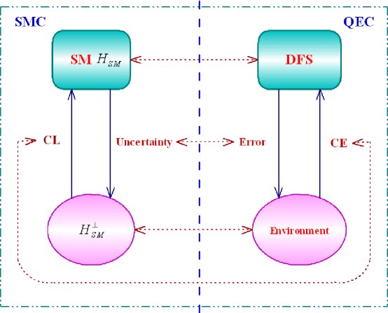
Figure 1: A representation of the relationships between sliding mode control (SMC) in QCP2 and a unified framework of quantum error correction (QEC). The sliding mode (SM $H_{SM}$) corresponds to the decoherence-free subspace (DFS); the complement space $H_{SM}^{\bot}$ corresponds to the effect of the environment in QEC; and the uncertainties in SMC correspond to possible errors in QEC. The subtask (I) in SMC corresponds to the initialization of QEC; the subtask (II) in SMC corresponds to the protection of DFS in QEC; and the control law (CL) in the subtask (III) of SMC corresponds to the process of correcting errors (CE) in QEC.

4.3 An illustrative example: three-level system

We now consider a three-level quantum system. In (3), let $u(t)=1$ and $A=\text{diag}\{-1,0,1\}$. The matrix $B$ and the uncertainty matrix $H_{\Delta}$ are as follows:

$$B=\left(\!\begin{array}[]{*{20}c}0&1&0\\ 1&0&0\\ 0&0&0\\ \end{array}\!\right),\ \ \ \ \ \ \ \ H_{\Delta}=\left(\!\begin{array}[]{*{20}c}0&0&\epsilon(t)\\ 0&0&0\\ \epsilon(t)&0&0\\ \end{array}\!\right),$$ (18)

where $|\epsilon(t)|\leq\bar{\epsilon}$. This leads to the following equation of the form (3)

$$i\left(\begin{array}[]{c}\dot{c}_{1}(t)\\ \dot{c}_{2}(t)\\ \dot{c}_{3}(t)\\ \end{array}\right)=\left(\begin{array}[]{ccc}-1&1&\epsilon(t)\\ 1&0&0\\ \epsilon(t)&0&1\\ \end{array}\right)\left(\begin{array}[]{c}c_{1}(t)\\ c_{2}(t)\\ c_{3}(t)\\ \end{array}\right).$$ (19)

The three eigenstates $\{|\phi_{1}\rangle,|\phi_{2}\rangle,|\phi_{3}\rangle\}$ are denoted as $\{|1\rangle,|2\rangle,|3\rangle\}$, respectively. Suppose that the initial state is $|1\rangle$; i.e., $\{c_{1}(0),c_{2}(0),c_{3}(0)\}=\{1,0,0\}$. The three-level system corresponding to (18) can be represented schematically as shown in Figure 2. The form of the $B$ matrix implies that there is a direct coupling between states $|1\rangle$ and $|2\rangle$. The form of the uncertainty matrix $H_{\Delta}$ implies that a disturbance coupling $\epsilon(t)$ exists between $|1\rangle$ and $|3\rangle$. It is easy to check using the method in Section 2.1 that the subspace spanned by $\{|1\rangle,|2\rangle\}$ can be used as a sliding mode; i.e., $S(|\psi\rangle,H)=1-(|\langle\psi|1\rangle|^{2}+|\langle\psi|2\rangle|^{2})=0$. Hence, our control problem may correspond to a practical problem in quantum information. For example, the two-level system with levels $|1\rangle$ and $|2\rangle$ can be used a qubit, and the uncertainty matrix $H_{\Delta}$ may represent a possible leakage into states outside the qubit subspace [68].

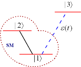
Figure 2: A three-level system. The subspace spanned by $\{|1\rangle,|2\rangle\}$ corresponds to the sliding mode (SM). The uncertainty $\epsilon(t)$ exists between $|1\rangle$ and $|3\rangle$.

We now consider the design of period $T$ for the periodic projective measurements. Let $c_{j}(t)=x_{j}(t)+iy_{j}(t)(j=1,2,3)$, where $x_{j}(t),y_{j}(t)\in\mathbf{R}$. Also, let the vector $\eta(t)$ denote $\eta(t)=(x_{1}(t),y_{1}(t),x_{2}(t),y_{2}(t),x_{3}(t),y_{3}(t))^{T}$. From (19), we obtain

$$\dot{\eta}(t)=F(\epsilon(t))\eta(t)$$ (20)

where

$$F(\epsilon(t))=\left(\begin{array}[]{cccccc}0&-1&0&1&0&\epsilon(t)\\ 1&0&-1&0&-\epsilon(t)&0\\ 0&1&0&&0&0\\ -1&0&0&0&0&0\\ 0&\epsilon(t)&0&0&0&1\\ -\epsilon(t)&0&0&0&-1&0\\ \end{array}\right),$$ (21)

and $\eta(0)=(x_{1}(0),y_{1}(0),x_{2}(0),y_{2}(0),x_{3}(0),y_{3}(0))^{T}=(1,0,0,0,0,0)^{T}$.

We now introduce the co-state vector $\mathbf{\lambda}(t)=(\lambda_{1}(t),\lambda_{2}(t),\lambda_{3}(t),\lambda_{4}(t),$ $\lambda_{5}(t),\lambda_{6}(t))^{T}$, and obtain the corresponding Hamiltonian function as follows:

$$\mathbb{H}({\eta(t),\epsilon(t),\mathbf{\lambda}(t),t})=\lambda^{T}(t)F(\epsilon(t))\eta(t)=\epsilon(t)M(t)+N(t),$$ (22)

where $M(t)=\lambda_{5}(t)y_{1}(t)-\lambda_{6}(t)x_{1}(t)-\lambda_{2}(t)x_{3}(t)+\lambda_{1}(t)y_{3}(t)$ and $N(t)=\lambda_{2}(t)x_{1}(t)-\lambda_{4}(t)x_{1}(t)-\lambda_{1}(t)y_{1}(t)+\lambda_{3}(t)y_{1}(t)-\lambda_{2}(t)x_{2}(t)+\lambda_{1}(t)y_{2}(t)-\lambda_{6}(t)x_{3}(t)+\lambda_{5}(t)y_{3}(t)$. According to Pontryagin’s minimum principle [69], a necessary condition for $\tilde{\epsilon}(t)$ to minimize the functional $J(\epsilon)=x_{3}^{2}(t_{f})+y_{3}^{2}(t_{f})$ is

$$\mathbb{H}({\tilde{\eta}(t),\tilde{\epsilon}(t),\tilde{\mathbf{\lambda}}(t),t})\leq\mathbb{H}({\tilde{\eta}(t),\epsilon(t),\tilde{\mathbf{\lambda}}(t),t}).$$ (23)

Hence,

$$\tilde{\epsilon}(t)=-\bar{\epsilon}\text{sgn}M(t).$$ (24)

That is, the optimal control is a bang-bang control strategy; i.e., $\tilde{\epsilon}(t)=\tilde{\epsilon}=+\bar{\epsilon}\ \text{or}-\bar{\epsilon}$.

Without loss of generality, now we let $\tilde{\epsilon}(t)=\bar{\epsilon}$ and focus on

$$\dot{\eta}(t)=F(\bar{\epsilon})\eta(t),$$ (25)

where $\eta(0)=(1,0,0,0,0,0)^{T}$.

Consider the optimal control with a fixed final time $t_{f}$ and a free final state $\eta(t_{f})=(x_{1}(t_{f}),y_{1}(t_{f}),x_{2}(t_{f}),y_{2}(t_{f}),x_{3}(t_{f}),y_{3}(t_{f}))^{T}$. Let $J(t)=x_{3}^{2}(t)+y_{3}^{2}(t)$. According to Pontryagin’s minimum principle, $\tilde{\lambda}(t_{f})=\frac{\partial}{\partial\eta}J(t)|_{t=t_{f}}$. From this, we obtain $(\lambda_{1}(t_{f}),\lambda_{2}(t_{f}),\lambda_{3}(t_{f}),\lambda_{4}(t_{f}),\lambda_{5}(t_{f}),\lambda_{6}(t_{f}))=(0,0,0,0,2x_{3}(t_{f}),2y_{3}(t_{f}))$. Now we consider another necessary condition $\dot{\lambda}(t)=-\frac{\partial\mathbb{H}({\eta(t),\epsilon(t),\mathbf{\lambda}(t),t})}{\partial\eta}$ which leads to the following relationships:

$$\dot{\mathbf{\lambda}}(t)=F(\bar{\epsilon})\lambda(t).$$ (26)

By simulation of (25) and (26), for different values of $\bar{\epsilon}$, we find the sign of $M(t)$ does not change over the first interval for which $J(t)$ is monotonically increasing with respect to $t$. Hence we can estimate the required period $T$ by considering the first interval on which $J(t)$ is monotonic. For example, if we consider $\bar{\epsilon}=0.1$, we obtain the simulation results shown in Figure 3. From this, we obtain $t_{f}=1.1160$, $x_{3}(t_{f})=-0.0055$, $y_{3}(t_{f})=-0.0705$ and $J(t_{f})=0.0050$.

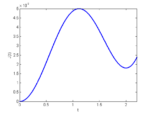
Figure 3: The curve of $J(t)=x_{3}^{2}(t)+y_{3}^{2}(t)$ corresponding to (25).

Then we can check that $M(t)$ indeed does not change sign on $t\in[0,t_{f}]$ as shown in Figure 4. Now we can design the period $T$ using the following relationship:

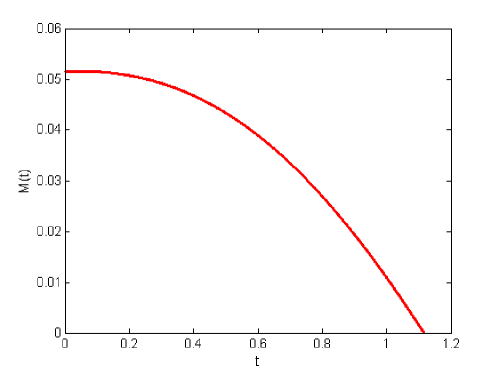
Figure 4: The curve of $M(t)$ corresponding to the first monotonic interval of $J(t)$ in Figure 3.

$$T=\left\{\!\begin{array}[]{ll}t_{1}\ (\text{where}\ t_{1}\in[0,t_{f})\ \text{and}\ J(t_{1})=p_{0})&\text{if}\ p_{0}<J(t_{f});\\ t_{f}&\text{otherwise}.\end{array}\right.$$ (27)

For example, if $p_{0}=0.50\%$, we have $p_{0}\leq J(t_{f})$. From Figure 3 and (27), we obtain $T=1.1160$.

Now we design a control law for the subtask (III) using the quantum amplitude amplification method introduced in Section 4.1. For simplicity, we use a simple choice of $\mathbf{Q}$ where $\varphi_{1}=\pi$, $\varphi_{2}=\pi$ and the subspace spanned by $\{|1\rangle,|2\rangle\}$ corresponds to the “good” subspace. When the measurement result is $|\phi_{k}\rangle=|3\rangle$, we first apply a unitary transformation (a perturbation) $\mathcal{U}_{3}$ on $|3\rangle$ to obtain $|\psi_{3}\rangle=\mathcal{U}_{3}|3\rangle=0.0600|1\rangle+0.0800|2\rangle+0.9950|3\rangle$. Now, using a similar method to the example in [52], we obtain the state $|\psi^{\prime}_{3}\rangle=0.5986|1\rangle+0.7981|2\rangle+0.0682|3\rangle$ after 7 iterations of $\mathbf{Q}$. Now we make a measurement on $|\psi^{\prime}_{3}\rangle$, and the probability of failure is $p^{\prime}_{0}=0.47\%$ ($\leq 0.50\%$).

5 Concluding remarks

This paper focuses on a robust control problem for quantum systems with uncertainties. The main contributions are as follows: (1) We propose a new robust control framework based on sliding mode control to deal with uncertainties in quantum control. Sliding mode control is a powerful methodology in classical control theory and has many industrial applications. Hence, the proposed method has the potential to open a new avenue for robust control design of quantum systems, which will provide a new useful tool for quantum information processing with uncertainties. (2) This paper presents two specific control algorithms for two classes of quantum control problems. In particular, several approaches such as time-optimal control, projective measurements and quantum amplitude amplification are combined to design quantum control algorithms. Two examples are also analyzed in detail using the proposed algorithms.

It should be pointed out that the results in this paper are only a first step in developing systematic sliding mode control approaches for quantum systems. Much further work is required and several open problems are listed as follows: (1) The measurement period $T$ designed in this paper is relatively conservative and it may be possible to obtain a larger value of $T$ when $p_{0}$ is relatively large. (2) The connection between the proposed methods and quantum error correction and quantum state preparation has been discussed. However, the specific applications still require to be developed in detail. Moreover, we use two model systems as the examples to illustrate the proposed methods. A future task is to connect such model systems to specific quantum systems (e.g., quantum optical systems and spin systems) and to consider the experimental implementation of the proposed methods for such real quantum systems. (3) We only consider a simple amplitude amplification operator $\mathbf{Q}$ in our example, and the questions of how to determine an optimal $\mathbf{Q}$ and how to realize $\mathbf{Q}$ using specific control fields are still open problems. (4) We have ignored the uncertainties during the control processes (I) and (III), which require a relatively short time to accomplish the two control objectives. An improvement worth exploring is to consider the effect of uncertainties in all three subtasks. (5) We have constrained the type of uncertainties to be dealt with, so future research could be directed forwards extending the sliding mode control approaches to deal with other types of uncertainties for quantum systems.

Appendix: The proof of Theorem 1

For $H=I_{z}+\epsilon(t)I_{x}$, using $\dot{\rho}=-i[H,\rho]$ and (9), we have

$$\left(\begin{array}[]{c}\dot{x}_{t}\\ \dot{y}_{t}\\ \dot{z}_{t}\\ \end{array}\right)=\left(\begin{array}[]{ccc}0&-1&0\\ 1&0&-\epsilon(t)\\ 0&\epsilon(t)&0\\ \end{array}\right)\left(\begin{array}[]{c}x_{t}\\ y_{t}\\ z_{t}\\ \end{array}\right),$$ (28)

where $(x_{0},y_{0},z_{0})=(0,0,1)$.

We now consider $\epsilon(t)$ as a control input and select the performance measure as

$$J(\epsilon)=z_{t_{f}}.$$ (29)

Also, we introduce the co-state vector $\lambda(t)=(\lambda_{1}(t),\lambda_{2}(t),\lambda_{3}(t))^{T}$ and obtain the corresponding Hamiltonian function as follows [69]:

$$\mathbb{H}({\mathbf{r}(t),\epsilon(t),\mathbf{\lambda}(t),t})=-\lambda_{1}(t)y_{t}+\lambda_{2}(t)x_{t}+\epsilon(t)(\lambda_{3}(t)y_{t}-\lambda_{2}(t)z_{t}).$$ (30)

According to Pontryagin’s minimum principle [69], a necessary condition for $\tilde{\epsilon}(t)$ to minimize $J(\epsilon)$ is

$$\mathbb{H}({\tilde{\mathbf{r}}(t),\tilde{\epsilon}(t),\mathbf{\tilde{\lambda}}(t),t})\leq\mathbb{H}({\tilde{\mathbf{r}}(t),\epsilon(t),\mathbf{\tilde{\lambda}}(t),t}).$$ (31)

Hence the optimal control $\tilde{\epsilon}(t)$ should be chosen as follows:

$$\tilde{\epsilon}(t)=-\bar{\epsilon}\text{sgn}(\lambda_{3}(t)y_{t}-\lambda_{2}(t)z_{t}).$$ (32)

That is, the optimal control strategy for $\epsilon(t)$ is bang-bang control; i.e., $\tilde{\epsilon}(t)=\tilde{\epsilon}=+\bar{\epsilon}\ \text{or}-\bar{\epsilon}$. Now we consider the system

$$\left(\begin{array}[]{c}\dot{x}_{t}\\ \dot{y}_{t}\\ \dot{z}_{t}\\ \end{array}\right)=\left(\begin{array}[]{ccc}0&-1&0\\ 1&0&-\tilde{\epsilon}\\ 0&\tilde{\epsilon}&0\\ \end{array}\right)\left(\begin{array}[]{c}x_{t}\\ y_{t}\\ z_{t}\\ \end{array}\right),$$ (33)

where $(x_{0},y_{0},z_{0})=(0,0,1)$. Define $\omega=\sqrt{1+\bar{\epsilon}^{2}}$. The corresponding solution to (33) is

$$\left(\begin{array}[]{c}x_{t}\\ y_{t}\\ z_{t}\\ \end{array}\right)=\left(\begin{array}[]{c}-\frac{\tilde{\epsilon}}{1+\bar{\epsilon}^{2}}\cos\omega t+\frac{\tilde{\epsilon}}{1+\bar{\epsilon}^{2}}\\ -\frac{\tilde{\epsilon}}{\sqrt{1+\bar{\epsilon}^{2}}}\sin\omega t\\ \frac{\bar{\epsilon}^{2}}{1+\bar{\epsilon}^{2}}\cos\omega t+\frac{1}{1+\bar{\epsilon}^{2}}\\ \end{array}\right).$$ (34)

Now consider the optimal control problem with a fixed final time $t_{f}$ and a free final state $\mathbf{r}_{t_{f}}=(x_{t_{f}},y_{t_{f}},z_{t_{f}})$. According to Pontryagin’s minimum principle, $\tilde{\lambda}(t_{f})=\frac{\partial}{\partial\mathbf{r}}z_{t}|_{t=t_{f}}$. From this, it is straightforward to verify that $(\lambda_{1}(t_{f}),\lambda_{2}(t_{f}),\lambda_{3}(t_{f}))=(0,0,1)$. Now let us consider another necessary condition $\dot{\lambda}(t)=-\frac{\partial\mathbb{H}({\mathbf{r}(t),\epsilon(t),\mathbf{\lambda}(t),t})}{\partial\mathbf{r}}$ which leads to the following relationships:

$$\dot{\mathbf{\lambda}}(t)=\left(\begin{array}[]{c}\dot{\lambda}_{1}(t)\\ \dot{\lambda}_{2}(t)\\ \dot{\lambda}_{3}(t)\\ \end{array}\right)=\left(\begin{array}[]{ccc}0&-1&0\\ 1&0&-\tilde{\epsilon}\\ 0&\tilde{\epsilon}&0\\ \end{array}\right)\left(\begin{array}[]{c}\lambda_{1}(t)\\ \lambda_{2}(t)\\ \lambda_{3}(t)\\ \end{array}\right),$$ (35)

where $(\lambda_{1}(t_{f}),\lambda_{2}(t_{f}),\lambda_{3}(t_{f}))=(0,0,1)$. The corresponding solution to (35) is

$$\left(\begin{array}[]{c}\lambda_{1}(t)\\ \lambda_{2}(t)\\ \lambda_{3}(t)\\ \end{array}\right)=\left(\begin{array}[]{c}-\frac{\tilde{\epsilon}}{1+\bar{\epsilon}^{2}}\cos\omega(t_{f}-t)+\frac{\tilde{\epsilon}}{1+\bar{\epsilon}^{2}}\\ \frac{\tilde{\epsilon}}{\sqrt{1+\bar{\epsilon}^{2}}}\sin\omega(t_{f}-t)\\ \frac{\bar{\epsilon}^{2}}{1+\bar{\epsilon}^{2}}\cos\omega(t_{f}-t)+\frac{1}{1+\bar{\epsilon}^{2}}\\ \end{array}\right).$$ (36)

We obtain

$$\lambda_{3}(t)y_{t}-\lambda_{2}(t)z_{t}=\frac{-\tilde{\epsilon}}{\omega^{3/2}}[\sin\omega t+\bar{\epsilon}^{2}\sin\omega t_{f}+\sin\omega(t_{f}-t)].$$ (37)

It is easy to show that the quantity $(\lambda_{3}(t)y_{t}-\lambda_{2}(t)z_{t})$ occurring in (32) does not change its sign when $t_{f}\in[0,\frac{\pi}{\sqrt{1+\bar{\epsilon}^{2}}}]$ and $t\in[0,t_{f}]$. That is to say, $\epsilon(t)=\tilde{\epsilon}$ is the optimal control when $t\in[0,\frac{\pi}{\sqrt{1+\bar{\epsilon}^{2}}}]$. Hence $z^{a}_{t}=z_{t}(\epsilon(t))\geq z_{t}(\tilde{\epsilon})=z^{b}_{t}$.

References

References

- [1] Warren W S, Rabitz H and Dahleh M 1993 Science 259 1581
- [2] Rabitz H, de Vivie-Riedle R, Motzkus M and Kompa K 2000 Science, 288 824
- [3] Chu S 2002 Nature 416 206
- [4] Rice S A and Zhao M S 2000 Optical Control of Molecular Dynamics (New York: John Wiley & Sons, Inc.)
- [5] Dantus M and Lozovoy V V 2004 Chem. Rev. 104 1813
- [6] Bonačić-Koutecký V and Mitrić R 2005 Chem. Rev. 105 11
- [7] Shapiro M and Brumer P 2003 Principles of the Quantum Control of Molecular Processes (New Jersey: John Wiley & Sons, Inc.)
- [8] Dowling J P and Milburn G J 2003 Phil. Trans. R. Soc. A 361 1655
- [9] Nielsen M A and Chuang I L 2000 Quantum Computation and Quantum Information (Cambridge, England: Cambridge University Press)
- [10] Santos L F and Viola L 2008 New J. Phys. 10 083009
- [11] Viola L and Lloyd S 1998 Phys. Rev. A 58 2733
- [12] Peirce A P, Dahleh M and Rabitz H 1988 Phys. Rev. A 37 4950
- [13] Khaneja N, Brockett R and Glaser S J 2001 Phys. Rev. A 63 032308
- [14] Wiseman H M and Milburn G J 1993 Phys. Rev. Lett. 70 548
- [15] Doherty A C, Habib S, Jacobs K, Mabuchi H and Tan S M 2000 Phys. Rev. A 62 012105
- [16] Lloyd S 2000 Phys. Rev. A 62 022108
- [17] van Handel R, Stockton J K and Mabuchi H 2005 J. Opt. B: Quantum Semiclass. Opt. 7 S179
- [18] van Handel R, Stockton J K and Mabuchi H 2005 IEEE Trans. Autom. Control 50 768
- [19] Mirrahimi M and van Handel R 2007 SIAM J. Control Optim. 46 445
- [20] Ahn C, Wiseman H M and Milburn G J 2003 Phys. Rev. A 67 052310
- [21] Mabuchi H 2008 Phys. Rev. A 78 032323
- [22] Yamamoto N, Nurdin H I, James M R and Petersen I R 2008 Phys. Rev. A 78 042339
- [23] Branderhorst M P A, Londero P, Wasylczyk P, Brif C, Kosut R L, Rabitz H and Walmsley I A 2008 Science 320 638
- [24] Brown E and Rabitz H 2002 J. Math. Chem. 31 17
- [25] Pravia M A, Boulant N, Emerson J, Fortunato E M, Havel T F, Cory D G and Farid A 2003 J. Chem. Phys. 119 9993
- [26] Zhang H and Rabitz H 1994 Phys. Rev. A 49 2241
- [27] Rabitz H 2002 Phys. Rev. A 66 063405
- [28] Bacon D, Lidar D A and Whaley K B 1999 Phys. Rev. A 60 1944
- [29] Viola L and Knill E 2003 Phys. Rev. Lett. 90 037901
- [30] Wesenberg J H 2004 Phys. Rev. A 69 042323
- [31] Stockton J K, Geremia J M, Doherty A C and Mabuchi H 2004 Phys. Rev. A 69 032109
- [32] Protopopescu V, Perez R, D’Helon C and Schmulen J 2003 J. Phys. A: Math. Gen. 36 2175
- [33] Duan L M, Lukin M D, Cirac J I and Zoller P 2001 Nature 414 413
- [34] Yamamoto N and Bouten L 2009 IEEE Trans. Autom. Control 54 92
- [35] D’Helon C and James M R 2006 Phys. Rev. A 73 053803
- [36] James M R, Nurdin H I and Petersen I R 2008 IEEE Trans. Autom. Control 53 1787
- [37] Utkin V I 1977 IEEE Trans. Autom. Control AC-22 212
- [38] Edwards C and Spurgeon S K 1998 Sliding Mode Control: Theory and Applications (London: Taylor & Francis)
- [39] Utkin V I, Guldner J and Shi J 1999 Sliding Mode Control in Electromechanical Systems (London: Taylor & Francis)
- [40] Dong D and Petersen I R 2009 Variable structure control of uncontrollable quantum systems, Proc. 6th IFAC Symposium on Robust Control Design (Haifa, Israel) 16
- [41] Vilela Mendes R and Man’ko V I 2003 Phys. Rev. A 67 053404
- [42] Turinici G and Rabitz H 2003 J. Phys. A: Math. Gen. 36 2565
- [43] Turinici G and Rabitz H 2001 Chem. Phys. 267 1
- [44] Tersigni S H, Gaspard P and Rice S A 1990 J. Chem. Phys. 93 1670
- [45] Dong D, Chen C, Tarn T J, Pechen A and Rabitz H 2008 IEEE Trans. Syst. Man Cybern.-Part B: Cybern. 38 957
- [46] Lidar D A, Chuang I L and Whaley K B 1998 Phys. Rev. Lett. 81 2594
- [47] Kwiat P G, Berglund A J, Altepeter J B and White A G 2000 Science 290 498
- [48] Schirmer S G, Fu H and Solomon A I 2001 Phys. Rev. A 63 063410
- [49] Gong J B and Rice S A 2004 J. Chem. Phys. 120 9984
- [50] Shuang F, Pechen A, Ho T S and Rabitz H 2007 J. Chem. Phys. 126 134303
- [51] Pechen A, Il’in N, Shuang F and Rabitz H 2006 Phys. Rev. A 74 052102
- [52] Dong D, Zhang C, Rabitz H, Pechen A and Tarn T J 2008 J. Chem. Phys. 129 154103
- [53] Roa L, Delgado A, Ladrón de Guevara M L and Klimov A B 2006 Phys. Rev. A 73 012322
- [54] Romano R and D’Alessandro D 2006 Phys. Rev. Lett. 97 080402
- [55] Romano R and D’Alessandro D 2006 Phys. Rev. A 73, 022323
- [56] Sugny D, Kontz C and Jauslin H R 2007 Phys. Rev. A 76 023419
- [57] Boscain U and Mason P 2006 J. Math. Phys. 47 062101
- [58] Itano W M, Heinzen D J, Bollinger J J and Wineland D J 1990 Phys. Rev. A 41 2295
- [59] Dong D, Lam J and Tarn T J 2009 IET Control Theory Appl. 3 161
- [60] Knill E, Laflamme R and Zurek W H 1998 Science 279 342
- [61] Brassard G, Høyer P and Tapp A 1998 Lect. Notes Comput. Sci. 1443 820
- [62] Høyer P 2000 Phys. Rev. A 62 052304
- [63] Grover L K 1998 Phys. Rev. Lett. 80 4329
- [64] Long G L 2001 Phys. Rev. A 64 022307
- [65] Wu R, Pechen A, Brif C and Rabitz H 2007 J. Phys. A: Math. Theor. 40 5681
- [66] Shor P W 1995 Phys. Rev. A 52 R2493
- [67] Steane A M 1996 Phys. Rev. Lett. 77 793
- [68] Devitt S J, Schirmer S G, Qi D K L, Cole J H and Hollenberg L C L 2007 New J. Phys. 9 384
- [69] Kirk D E 1970 Optimal Control Theory: An Introduction (New Jersey: Prentice-Hall Inc.)