The embedded contact homology of sutured solid tori

Abstract.

We calculate the relative versions of embedded contact homology, contact homology and cylindrical contact homology of the sutured solid torus $(S^{1}\times D^{2},\Gamma)$, where $\Gamma$ consists of $2n$ parallel longitudinal sutures.

1. Introduction

The embedded contact homology (ECH) of a closed, oriented $3$-manifold with a contact form was introduced by Hutchings in [9, 10, 11, 12] and is a variant of the symplectic field theory [6] of Eliashberg, Givental and Hofer. It is defined in terms of a contact form but is an invariant of the underlying $3$-manifold. This invariance has been established by Taubes in [19, 20] via the identification with Seiberg-Witten Floer (co-)homology as defined by Kronheimer and Mrowka [17] and in particular implies the Weinstein conjecture in dimension three. ECH is also conjecturally isomorphic to Ozsváth–Szabó Heegaard Floer homology defined in [18]. We would like to mention that Kutluhan, Lee and Taubes, and independently Colin, Ghiggini and Honda have recently announced two different proofs of the isomorphism between Hutchings’s embedded contact homology and Heegaard Floer homology.

A natural condition to impose on a compact, oriented contact $(2m+1)$-manifold $(M,\xi)$ with boundary is to require that $\partial M$ be convex, i.e., there is a contact vector field $X$ transverse to $\partial M$. To a transverse contact vector field $X$ we can associate the dividing set $\Gamma=\Gamma_{X}\subset\partial M$, namely the set of points $x\in\partial M$ such that $X(x)\in\xi(x)$. By the contact condition, $(\Gamma,\xi\cap T\Gamma)$ is a $(2m-1)$-dimensional contact submanifold of $(M,\xi)$; the isotopy class of $(\Gamma,\xi\cap T\Gamma)$ is independent of the choice of $X$. We will denote by $(M,\Gamma,\xi)$ the contact manifold $(M,\xi)$ with convex boundary and dividing set $\Gamma=\Gamma_{X}\subset\partial M$ with respect to some transverse contact vector field $X$. Note that the actual boundary condition we need is slightly different and is called a sutured boundary condition. (In the early 1980’s, Gabai developed the theory of sutured manifolds [8], which became a powerful tool in studying $3$-manifolds with boundary.) For the moment we write $(M,\Gamma,\xi)$ to indicate either the convex boundary condition or the sutured boundary condition.

It turns out that there is a way to generalize embedded contact homology to sutured $3$-manifolds. This is possible by imposing a certain convexity condition on the contact form. This construction is completely described in the paper of Colin, Ghiggini, Honda and Hutchings [3]. Heegaard Floer homology also admits a sutured version, namely the sutured Floer homology (SFH) of Juhász [13, 14], which is an invariant of sutured manifolds. Finally, Kronheimer and Mrowka in [16] introduced the sutured version of Seiberg-Witten Floer homology.

Extending the conjectured equivalence of Heegaard Floer homology and embedded contact homology, the following conjecture was formulated in [3]:

Conjecture 1.1.

$SFH(-M,-\Gamma,\mathfrak{s}_{\xi}+PD(h))\simeq ECH(M,\Gamma,\xi,h)$, where $\mathfrak{s}_{\xi}$ denotes the relative Spin^c-structure determined by $\xi$ and $h\in H_{1}(M;\mathbb{Z})$.

In this paper, we construct sutured contact solid torus with $2n$ parallel longitudinal sutures, where $n\geq 2$, using the gluing method of Colin, Ghiggini, Honda and Hutchings [3] and calculate the sutured embedded contact homology of it. We apply the gluing method in such a way that the constructed sutured solid torus is equipped with a nondegenerate contact form satisfying the property that all closed embedded Reeb orbits are noncontractible, define the same homology class and have the same symplectic action. It turns out that for the constructed sutured manifolds the sutured version of embedded contact homology coincides with sutured Floer homology. The corresponding calculation in sutured Floer homology has been done by Juhász in [15]. So far, this is the first series of nontrivial examples where these two theories provide the same answer.

Theorem 1.2.

Let $(S^{1}\times D^{2},\Gamma)$ be a sutured manifold, where $\Gamma$ is a set of $2n$ parallel longitudinal curves and $n\geq 2$. Then there is a contact form $\alpha$ which makes $(S^{1}\times D^{2},\Gamma)$ a sutured contact manifold and

$$ECH(S^{1}\times D^{2},\Gamma,\alpha,J,h)\simeq\left\{\begin{array}[]{ll}\mathbb{Z}^{n-1\choose h},&\mbox{for}\ 0\leq h\leq n-1;\\ 0,&\mbox{otherwise},\end{array}\right.$$

where $h\in H_{1}(S^{1}\times D^{2};\mathbb{Z})$ and $J$ is an adapted almost complex structure. Hence,

$$ECH(S^{1}\times D^{2},\Gamma,\alpha,J)=\bigoplus\limits_{h\in H_{1}(S^{1}\times D^{2};\mathbb{Z})}ECH(S^{1}\times D^{2},\Gamma,\alpha,J,h)\simeq\mathbb{Z}^{2^{n-1}}.$$

There is a Floer-type invariant of a closed, oriented contact odd-dimensional manifold, called contact homology. Contact homology was introduced by Eliashberg and Hofer and is a special case of the symplectic field theory. In [3], Colin, Ghiggini, Honda and Hutchings generalized contact homology to sutured manifolds.

For the sutured contact manifold from Theorem 1.2, we calculated the sutured versions of cylindrical contact homology and contact homology.

Theorem 1.3.

Let $(S^{1}\times D^{2},\Gamma,\alpha)$ be a sutured contact manifold from Theorem 1.2. Then $HC^{cyl}(S^{1}\times D^{2},\Gamma,\alpha)$ is defined, is independent of the contact form $\alpha$ for the given contact structure $\xi$ and almost complex structure $J$,

$$HC^{cyl,h}(S^{1}\times D^{2},\Gamma,\xi) =\bigoplus\limits_{i\in\mathbb{Z}}HC^{cyl,h}_{i}(S^{1}\times D^{2},\Gamma,\xi)$$

$$\simeq\left\{\begin{array}[]{ll}\mathbb{Q}^{n-1},&\mbox{for}\ h\geq 1;\\ 0,&\mbox{otherwise},\end{array}\right.$$

and hence

$$HC^{cyl}(S^{1}\times D^{2},\Gamma,\xi)=\bigoplus\limits_{h\geq 1}\bigoplus\limits_{i\in\mathbb{Z}}HC^{cyl,h}_{i}(S^{1}\times D^{2},\Gamma,\xi)\simeq\bigoplus\limits_{h\geq 1}\mathbb{Q}^{n-1},$$

where $h$ is the homological grading and $i$ is the Conley-Zehnder grading.

Theorem 1.4.

Let $(S^{1}\times D^{2},\Gamma,\alpha)$ be a sutured contact manifold from Theorem 1.2. Then $HC(S^{1}\times D^{2},\Gamma,\alpha)$ is defined, is independent of the contact form $\alpha$ for the given contact structure $\xi$ and almost complex structure $J$,

$$HC^{h}(S^{1}\times D^{2},\Gamma,\xi)=\bigoplus\limits_{i\in\mathbb{Z}}HC^{h}_{i}(S^{1}\times D^{2},\Gamma,\xi)\simeq\mathbb{Q}^{\rho(n,h)}$$

and hence

$$HC(S^{1}\times D^{2},\Gamma,\xi)=\bigoplus\limits_{h\in\mathbb{Z}}\bigoplus\limits_{i\in\mathbb{Z}}HC^{h}_{i}(S^{1}\times D^{2},\Gamma,\xi)\simeq\bigoplus\limits_{h\in\mathbb{Z}}\mathbb{Q}^{\rho(n,h)},$$

where $h$ is the homological grading, $i$ is the Conley-Zehnder grading and $\rho(n,h)$ denotes the coefficient of $x^{h}$ in the generating function $\prod^{\infty}_{s=1}(1+x^{s})^{n-1}$.

This paper is organized as follows: in Section 2 we review definitions of embedded contact homology, cylindrical contact homology and contact homology for sutured contact manifolds; Section 3 describes the construction of sutured contact solid torus with $2n$ longitudinal sutures, where $n\geq 2$; finally in Section 4 we calculate the relative versions of embedded contact homology, cylindrical contact homology and contact homology of the solid torus constructed in Section 3.

2. Background

The goal of this section is to review definitions of embedded contact homology, cylindrical contact homology and contact homology for contact sutured manifolds. This section is essentially a summary of [3].

2.1. Sutured contact manifolds

In this section we repeat some definitions from [3].

Definition 2.1.

A Liouville manifold (often also called a Liouville domain) is a pair $(W,\beta)$ consisting of a compact, oriented $2n$-dimensional manifold $W$ with boundary and a $1$-form $\beta$ on $W$, where $\omega=d\beta$ is a positive symplectic form on $W$ and the Liouville vector field $Y$ given by $i_{Y}(\omega)=\beta$ is positively transverse to $\partial W$. It follows that the $1$-form $\beta_{0}=\beta|_{\partial W}$ (this notation means $\beta$ pulled back to $\partial W$) is a positive contact form with kernel $\zeta$.

Definition 2.2.

A compact oriented $m$-dimensional manifold $M$ with boundary and corners is a sutured manifold if it comes with an oriented, not necessarily connected submanifold $\Gamma\subset\partial M$ of dimension $m-2$ (called the suture), together with a neighborhood $U(\Gamma)=[-1,0]\times[-1,1]\times\Gamma$ of $\Gamma=\{0\}\times\{0\}\times\Gamma$ in $M$, with coordinates $(\tau,t)\in[-1,0]\times[-1,1]$, such that the following holds:

• $U\cap\partial M=(\{0\}\times[-1,1]\times\Gamma)\cup([-1,0]\times\{-1\}\times\Gamma)\cup([-1,0]\times\{1\}\times\Gamma)$;

• $\partial M\setminus(\{0\}\times(-1,1)\times\Gamma)=R_{-}(\Gamma)\sqcup R_{+}(\Gamma)$, where the orientation of $\partial M$ agrees with that of $R_{+}(\Gamma)$ and is opposite that of $R_{-}(\Gamma)$, and the orientation of $\Gamma$ agrees with the boundary orientation of $R_{+}(\Gamma)$;

• the corners of $M$ are precisely $\{0\}\times\{\pm 1\}\times\Gamma$.

The submanifold $\partial_{h}M=R_{+}(\Gamma)\cup R_{-}(\Gamma)$ is called the horizontal boundary and $\partial_{v}M=\{0\}\times[-1,1]\times\Gamma$ the vertical boundary of $M$.

Definition 2.3.

Let $(M,\Gamma,U(\Gamma))$ be a sutured manifold. If $\xi$ is a contact structure on $M$ (this means that $M$ is now $2n+1$-dimensional), we say that $(M,\Gamma,U(\Gamma),\xi)$ is a sutured contact manifold if $\xi$ is the kernel of a positive contact 1-form $\alpha$ such that:

• $(R_{+}(\Gamma),\beta_{+}=\alpha|_{R_{+}(\Gamma)})$ and $(R_{-}(\Gamma),\beta_{-}=\alpha|_{R_{-}(\Gamma)})$ are Liouville manifolds;

• $\alpha=Cdt+\beta$ inside $U(\Gamma)$, where $C>0$ and $\beta$ is independent of $t$ and does not have a $dt$-term;

• $\partial_{\tau}=Y_{\pm}$, where $Y_{\pm}$ is a Liouville vector field for $\beta_{\pm}$.

Such a contact form is said to be adapted to $(M,\Gamma,U(\Gamma))$.

2.2. Completion of a sutured contact manifold

Let $(M,\Gamma,U(\Gamma),\xi)$ be a sutured contact manifold with an adapted contact form $\alpha$. The form $\alpha$ is then given by $Cdt+\beta_{\pm}$ on the neighborhoods $[1-\varepsilon,1]\times R_{+}(\Gamma)$ and $[-1,-1+\varepsilon]\times R_{-}(\Gamma)$ of $R_{+}(\Gamma)=\{1\}\times R_{+}(\Gamma)$ and $R_{-}(\Gamma)=\{-1\}\times R_{-}(\Gamma)$, where $t\in[-1,-1+\varepsilon]\cup[1-\varepsilon,1]$ extends the $t$-coordinate on $U$. On $U$, $\alpha=Cdt+\beta$, $\beta=\beta_{+}=\beta_{-}$, and $\partial_{\tau}$ is a Liouville vector field $Y$ for $\beta$.

Following the procedure explained in [3] we can “complete” $(M,\alpha)$ to a noncompact contact manifold $(M^{\ast},\alpha^{\ast})$. We first extend $\alpha$ to $[1,\infty)\times R_{+}(\Gamma)$ and $(-\infty,-1]\times R_{-}(\Gamma)$ by taking $Cdt+\beta_{\pm}$ as appropriate. The boundary of this new manifold is $\{0\}\times\mathbb{R}\times\Gamma$. Notice that since $\partial_{\tau}=Y$, the form $d\beta|_{[-1,0]\times\{t\}\times\Gamma}$ is the symplectization of $\beta|_{\{0\}\times\{t\}\times\Gamma}$ in the positive $\tau$-direction. We glue $[0,\infty)\times\mathbb{R}\times\Gamma$ with the form $Cdt+e^{\tau}\beta_{0}$, where $\beta_{0}$ is the pullback of $\beta$ to $\{0\}\times\{t\}\times\Gamma$.

Let $M^{\ast}$ be the noncompact extension of $M$ described above and $\alpha^{\ast}$ be the extension of $\alpha$ to $M^{\ast}$. For convenience, we extend the coordinates $(\tau,t)$ – so far defined only on the ends of $M^{\ast}$ – to functions on $M^{\ast}$ so that $t(M)\subset[-1,1]$ and $\tau(M)\subset[-1,0]$. We then say that $t>1$ corresponds the Top (T), $t<-1$ corresponds to the Bottom (B), and $\tau>0$ corresponds to the Side (S). Let $(\widehat{R_{\pm}(\Gamma)},\widehat{\beta}_{\pm})$ be the extension/completion of $(R_{\pm}(\Gamma),\beta_{\pm})$, obtained by extending to (S).

2.3. Reeb orbits and Conley-Zehnder index

Let $(M,\Gamma,U(\Gamma),\xi)$ be a sutured contact manifold with an adapted contact form $\alpha$ and $(M^{\ast},\alpha^{\ast})$ be its completion.

The Reeb vector field $R_{\alpha^{\ast}}$ that is associated to a contact form $\alpha^{\ast}$ is characterized by

$$\left\{\begin{array}[]{ll}d\alpha^{\ast}(R_{\alpha^{\ast}},\cdot)=0;\\ \alpha^{\ast}(R_{\alpha^{\ast}})=1.\end{array}\right.$$

A Reeb orbit is a closed orbit of the Reeb flow, i.e., a smooth map $\gamma\colon\thinspace\mathbb{R}/T\mathbb{Z}\to M$ for some $T>0$ such that $\dot{\gamma}(t)=R_{\alpha^{\ast}}(\gamma(t))$.

Remark 2.4.

Every periodic orbit of $R_{\alpha^{\ast}}$ lies in $M$. Hence, the set of periodic Reeb orbits of $R_{\alpha^{\ast}}$ coincides with the set of periodic Reeb orbits of $R_{\alpha}$.

Consider Reeb orbit $\gamma$ passing through a point $x\in M$. The linearization of the Reeb flow on the contact planes along $\gamma$ determines a linearized return map $P_{\gamma}\colon\thinspace\xi_{x}\to\xi_{x}$. This linear map is symplectic and it does not depend on $x$ (up to conjugation). The Reeb orbit $\gamma$ is nondegenerate if $1\notin Spec(P_{\gamma})$.

Note that nondegeneracy can always be achieved by a small perturbation, i.e., for any contact structure $\xi$ on $M$, there exists a contact form $\alpha$ for $\xi$ such that all closed orbits of $R_{\alpha}$ are nondegenerate.

For simplicity, we assume that all Reeb orbits of $R_{\alpha}$, including multiply covered ones, are nondegenerate.

A Reeb orbit $\gamma$ is called elliptic or positive (respectively negative) hyperbolic if the eigenvalues of $P_{\gamma}$ are on the unit circle or the positive (resp. negative) real line respectively.

If $\tau$ is a trivialization of $\xi$ over $\gamma$, we can then define the Conley-Zehnder index. In $3$-dimensional situation this is given explicitly as follows:

Proposition 2.5 ([9]).

If $\gamma$ is elliptic, then there is an irrational number $\phi\in\mathbb{R}$ such that $P_{\gamma}$ is conjugate in $SL_{2}(\mathbb{R})$ to a rotation by angle $2\pi\phi$, and

$$\mu_{\tau}(\gamma^{k})=2\lfloor k\phi\rfloor+1,$$

where $2\pi\phi$ is the total rotation angle with respect to $\tau$ of the linearized flow around the orbit.

If $\gamma$ is positive (respectively negative) hyperbolic, then there is an even (respectively odd) integer $r$ such that the linearized flow around the orbit rotates the eigenspaces of $P_{\gamma}$ by angle $\pi r$ with respect to $\tau$, and

$$\mu_{\tau}(\gamma^{k})=kr.$$

2.4. Almost complex structure

In this section we repeat some definitions from Section 3.1 in [3].

Definition 2.6.

Let $(M,\xi)$ be a contact manifold with a contact form $\alpha$ such that $\xi=ker(\alpha)$. An almost complex structure $J$ on the symplectization $\mathbb{R}\times M$ is $\alpha$-adapted if $J$ is $\mathbb{R}$-invariant; $J(\xi)=\xi$ with $d\alpha(v,Jv)>0$ for nonzero $v\in\xi$; and $J(\partial_{s})=R_{\alpha}$, where $s$ denotes the $\mathbb{R}$-coordinate and $R_{\alpha}$ is a Reeb vector field associated to $\alpha$.

Definition 2.7.

Let $(W,\beta)$ be a Liouville manifold and $\zeta$ be the contact structure given on $\partial W$ by $ker(\beta_{0})$, where $\beta_{0}=\beta|_{\partial W}$. In addition, let $(\widehat{W},\widehat{\beta})$ be the completion of $(W,\beta)$, i.e., $\widehat{W}=W\cup([0,\infty)\times\partial W)$ and $\widehat{\beta}|_{[0,\infty)\times\partial W}=e^{\tau}\beta_{0}$, where $\tau$ is the $[0,\infty)$-coordinate. An almost complex structure $J_{0}$ on $\widehat{W}$ is $\widehat{\beta}$- adapted if $J_{0}$ is $\beta_{0}$-adapted on $[0,\infty)\times\partial W$; and $d\beta(v,J_{0}v)>0$ for all nonzero tangent vectors $v$ on $W$.

Definition 2.8.

Let $(M,\Gamma,U(\Gamma),\xi)$ be a sutured contact manifold, $\alpha$ be an adapted contact form and $(M^{\ast},\alpha^{\ast})$ be its completion. We say that an almost complex structure $J$ on $\mathbb{R}\times M^{\ast}$ is tailored to $(M^{\ast},\alpha^{\ast})$ if the following hold:

• $J$ is $\alpha^{\ast}$-adapted;

• $J$ is $\partial_{t}$-invariant in a neighborhood of $M^{\ast}\setminus int(M)$;

• The projection of $J$ to $T\widehat{R_{\pm}(\Gamma)}$ is a $\widehat{\beta}_{\pm}$-adapted almost complex structure $J_{0}$ on the completion $(\widehat{R_{+}(\Gamma)},\widehat{\beta}_{+})\bigsqcup(\widehat{R_{-}(\Gamma)},\widehat{\beta}_{-})$ of the Liouville manifold $(R_{+}(\Gamma),\beta_{+})\bigsqcup(R_{-}(\Gamma),\beta_{-})$. Moreover, the flow of $\partial_{t}$ identifies $J_{0}|_{\widehat{R_{+}(\Gamma)}\setminus R_{+}(\Gamma)}$ and $J_{0}|_{\widehat{R_{-}(\Gamma)}\setminus R_{-}(\Gamma)}$.

2.5. Sutured embedded contact homology

First, let $M$ be a closed, oriented $3$-manifold, $\alpha$ be a contact $1$-form on $M$ and let $J$ be an $\alpha$-adapted almost complex structure on $\mathbb{R}\times M$. For simplicity, we assume that all Reeb orbits of $R_{\alpha}$, including multiply covered ones, are nondegenerate.

Definition 2.9.

An orbit set is a finite set of pairs $a=\{(\alpha_{i},m_{i})\}$, where the $\alpha_{i}$’s are distinct embedded orbits of $R_{\alpha}$ and the $m_{i}$’s are positive integers. The orbit set $a$ is admissible if $m_{i}=1$ whenever $\alpha_{i}$ is hyperbolic. The homology class of $a$ is defined by

$$[a]:=\sum\limits_{i}m_{i}[\alpha_{i}]\in H_{1}(M;\mathbb{Z}).$$

If $a=\{(\alpha_{i},m_{i})\}$ and $b=\{(\beta_{j},n_{j})\}$ are two orbit sets with $[a]=[b]$, let $H_{2}(M,a,b)$ denote the set of relative homology classes of $2$-chains $Z$ in $M$ with

$$\partial Z=\sum\limits_{i}m_{i}\alpha_{i}-\sum\limits_{j}n_{i}\beta_{j}.$$

Definition 2.10.

The ECH chain complex $C_{\ast}(M,\alpha,h)$ is a free $\mathbb{Z}$-module with one generator for each admissible orbit set $a$ with $[a]=h$.

Definition 2.11.

If $a=\{(\alpha_{i},m_{i})\}$ and $b=\{(\beta_{j},n_{j})\}$ are orbit sets with $[a]=[b]$, let $\mathcal{M}^{J}(a,b)$ denote the moduli space of $J$-holomorphic curves $u$ with positive ends at covers of $\alpha_{i}$ with total multiplicity $m_{i}$, negative ends at covers of $\beta_{j}$ with total multiplicity $n_{j}$ , and no other ends. Note that the projection of each $u\in\mathcal{M}^{J}(a,b)$ to $M$ has a well-defined relative homology class $[u]\in H_{2}(M,a,b)$. For $Z\in H_{2}(M,a,b)$ we then define

$$M^{J}(a,b,Z):=\{u\in M^{J}(a,b)|\ [u]=Z\}.$$

Definition 2.12.

If $a=\{(\alpha_{i},m_{i})\}$ is an orbit set, define the symplectic action

$$\mathcal{A}(a):=\sum\limits_{i}m_{i}\int\limits_{\alpha_{i}}\alpha.$$

Lemma 2.13 ([10]).

For an adapted almost complex structure $J$, if $M^{J}(a,b)$ is non-empty, then:

• $\mathcal{A}(a)\geq\mathcal{A}(b)$.

• If $\mathcal{A}(a)=\mathcal{A}(b)$, then $a=b$ and every element of $\mathcal{M}^{J}(a,b)$ maps to a union of trivial cylinders.

Definition 2.14.

If $u\in\mathcal{M}^{J}(a,b,Z)$, define the ECH index

$$I(u)=I(a,b,Z)=c_{1}(\xi|_{Z},\tau)+Q_{\tau}(Z)+\sum\limits_{i}\sum\limits_{k=1}^{m_{i}}\mu_{\tau}(\alpha_{i}^{k})-\sum\limits_{j}\sum\limits_{k=1}^{n_{j}}\mu_{\tau}(\beta_{j}^{k}).$$

Here $Q_{\tau}(Z)$ denotes the relative intersection pairing, which is defined in [9].

Any $J$-holomorphic curve $u\in M^{J}(a,b)$ can be uniquely written as $u=u_{0}\cup u_{1}$, where $u_{0}$ and $u_{1}$ are unions of components of $u$, each component of $u_{0}$ maps to an $\mathbb{R}$-invariant cylinder, and no component of $u_{1}$ does.

Proposition 2.15 ([11]).

Suppose that $J$ is generic and $u=u_{0}\cup u_{1}\in\mathcal{M}^{J}(a,b)$. Then:

• $I(u)\geq 0$ with equality if and only if $u=u_{0}$.

• If $I(u)=1$, then $u$ contains one embedded component $u_{1}$ with $ind(u_{1})=I(u_{1})=1$ and $u_{0}$ does not intersect $u_{1}$.

To fix the signs in the differential, fix some ordering of all the embedded positive hyperbolic Reeb orbits in $M$.

Two curves $u$ and $u^{\prime}$ in $\mathcal{M}^{J}(a,b,Z)/\mathbb{R}$ are equivalent if their embedded components $u_{1}$ and $u^{\prime}_{1}$ are the same up to translation, and if their other components cover each embedded trivial cylinder $\mathbb{R}\times\gamma$ with the same total multiplicity. The differential $\partial$ in $ECH$ counts $I=1$ curves in $M^{J}(a,b)/\mathbb{R}$ where $a$ and $b$ are admissible orbit sets. Such curves may contain multiple covers of the $\mathbb{R}$-invariant cylinder $\mathbb{R}\times\gamma$ when $\gamma$ is an elliptic embedded Reeb orbit. The differential $\partial$ only keeps track of the total multiplicity of such coverings for each $\gamma$. Finiteness of the count results from the ECH compactness theorem [9, Lemma 9.8]. For the sign of the count we refer to [12].

Let $(M,\Gamma,U(\Gamma),\xi)$ be a sutured contact $3$-manifold with an adapted contact form $\alpha$, $(M^{\ast},\alpha^{\ast})$ be its completion and $J$ be an almost complex structure on $\mathbb{R}\times M^{\ast}$ which is tailored to $(M^{\ast},\alpha^{\ast})$.

The sutured embedded contact homology group $ECH(M,\Gamma,\alpha,J)$ is defined to be the embedded contact homology of $(M^{\ast},\alpha^{\ast},J)$.

The following theorems have been proven by Colin, Ghiggini, Honda and Hutchings in [3]:

Theorem 2.16 ([3]).

The ECH compactness theorem [9, Lemma 9.8] holds for $J$-holomorphic curves in the symplectization of the completion of a sutured contact $3$-manifold, provided that we choose the almost complex structure $J$ on $\mathbb{R}\times M^{\ast}$ to be tailored to $(M^{\ast},\alpha^{\ast})$.

Theorem 2.17 ([3]).

Let $(M,\Gamma,U(\Gamma),\xi)$ be a sutured contact $3$-manifold with an adapted contact form $\alpha$, $(M^{\ast},\alpha^{\ast})$ be its completion and $J$ be an almost complex structure on $\mathbb{R}\times M^{\ast}$ which is tailored to $(M^{\ast},\alpha^{\ast})$. Then the embedded contact homology group $ECH(M,\Gamma,\alpha,J)$ is defined.

Remark 2.18.

Lemma 2.13 and Proposition 2.15 hold for $J$-holomorphic curves in the symplectization of the completion of a sutured contact manifold, provided that we choose the almost complex structure $J$ on $\mathbb{R}\times M^{\ast}$ to be tailored to $(M^{\ast},\alpha^{\ast})$.

Recall that embedded contact homology is an invariant of the underlying closed, oriented $3$-manifold. Hence, it is natural to expect the following:

Conjecture 2.19 ([3]).

The embedded contact homology group $ECH(M,\Gamma,\alpha,J)$ does not depend on the choice of contact form $\alpha$, contact structure $\xi=ker(\alpha)$, and almost complex structure $J$.

2.6. Sutured contact homology

Let $(M,\Gamma,U(\Gamma),\xi)$ be a sutured contact manifold with an adapted contact form $\alpha$, $(M^{\ast},\alpha^{\ast})$ be its completion and $J$ be an almost complex structure on $\mathbb{R}\times M^{\ast}$ which is tailored to $(M^{\ast},\alpha^{\ast})$. For simplicity, we assume that all Reeb orbits of $R_{\alpha}$, including multiply covered ones, are nondegenerate.

Let $\gamma$ be an embedded Reeb orbit. We are also interested in the multiple covers $\gamma^{m}$ of $\gamma$, $m\geq 2$. There are 2 ways the Conley-Zehnder index of $\gamma^{m}$ can behave :

• the parity of $\mu_{\tau}(\gamma^{m})$ is the same for all $m\geq 1$.

• the parity for the even multiples $\mu_{\tau}(\gamma^{2k})$, $k\geq 1$, disagrees with the parity for the odd multiples $\mu_{\tau}(\gamma^{2k-1})$, $k\geq 1$.

In the second case, the even multiples $\gamma^{2k}$, $k\geq 1$, are called bad orbits. An orbit that is not bad is called good.

The sutured contact homology algebra $HC(M,\Gamma,\alpha,J)$ is defined to be the contact homology of $(M^{\ast},\alpha^{\ast},J)$ in the following sense: The contact homology chain complex $\mathcal{A}(\alpha,J)$ is the free supercommutative $\mathbb{Q}$-algebra with unit generated by good Reeb orbits, where the grading and the boundary map $\partial$ are defined in the usual way (as in [6]) with respect to the $\alpha^{\ast}$-adapted almost complex structure $J$. The homology of $\mathcal{A}(\alpha,J)$ is the sutured contact homology algebra $HC(M,\Gamma,\alpha,J)$.

We define the sutured cylindrical contact homology group $HC^{cyl}(M,\Gamma,\alpha,J)$ to be the cylindrical contact homology of $(M^{\ast},\alpha^{\ast},J)$. The cylindrical contact homology chain complex $C(\alpha,J)$ is the $\mathbb{Q}$-module freely generated by all good Reeb orbits, where the grading and the boundary map $\partial$ are defined as in [1] with respect to the $\alpha^{\ast}$-adapted almost complex structure $J$. The homology of $C(\alpha,J)$ is the sutured cylindrical contact homology group $HC^{cyl}(M,\Gamma,\alpha,J)$.

For our calculations we will need the following fact which is a consequence of Lemma 5.4 in [2]:

Fact 2.20 ([2]).

Let $(M,\alpha)$ be a closed, oriented contact manifold with nondegenerate Reeb orbits and

$$u=(a,f)\colon\thinspace(\dot{S},j)\to(\mathbb{R}\times M,J)$$

be a $J$-holomorphic curve in $\mathcal{M}^{J}(\gamma;\gamma_{1},\dots,\gamma_{s})$, where $\gamma$ and $\gamma_{i}$’s are all good Reeb orbits, $J$ is an $\alpha$-adapted almost complex structure on $\mathbb{R}\times M$ and $M^{J}(\gamma;\gamma_{1},\dots,\gamma_{s})$ is a moduli space of $J$-holomorphic curves that we consider in contact homology. Then

$$\mathcal{A}(u)=\mathcal{A}(\gamma)-\sum\limits_{i=1}^{s}\mathcal{A}(\gamma_{i})=\int\limits_{\gamma}\alpha-\sum\limits_{i=1}^{s}\int\limits_{\gamma_{i}}\alpha\geq 0$$

with equality if and only if the image of $f$ is contained in a trajectory of $R_{\alpha}$, i.e., $u$ maps to a trivial cylinder over $\tilde{\gamma}$, where $\tilde{\gamma}$ is an embedded orbit of $R_{\alpha}$, and hence $\gamma=\tilde{\gamma}^{k}$ for some $k$ and $\gamma_{i}=\tilde{\gamma}^{k_{i}}$ with $\sum_{i=1}^{s}k_{i}=k$.

In addition, we recall the following fact proven by Eliashberg and Hofer:

Fact 2.21 ([1]).

Let $(M,\alpha)$ be a closed, oriented contact manifold with nondegenerate Reeb orbits. Let $C_{i}^{h}(M,\alpha)$ be the cylindrical contact homology complex, where $h$ is a homotopy class of Reeb orbits and $i$ corresponds to the Conley-Zehnder grading. If there are no contractible Reeb orbits, then for every free homotopy class $h$

• $\partial^{2}=0$;

• $H(C^{h}_{\ast}(M,\alpha),\partial)$ is independent of the contact form $\alpha$ for $\xi$, the almost complex structure $J$ and the choice of perturbation for the moduli spaces.

Now we remind the following theorems which have been proven by Colin, Ghiggini, Honda and Hutchings in [3]:

Theorem 2.22 ([3]).

The SFT compactness theorem [2, Theorem 10.1] holds for $J$-holomorphic curves in the symplectization of the completion of a sutured contact manifold, provided that we choose the almost complex structure $J$ on $\mathbb{R}\times M^{\ast}$ to be tailored to $(M^{\ast},\alpha^{\ast})$.

Theorem 2.23 ([3]).

Let $(M,\Gamma,U(\Gamma),\xi)$ be a sutured contact $3$-manifold with an adapted contact form $\alpha$, $(M^{\ast},\alpha^{\ast})$ be its completion and $J$ be an almost complex structure on $\mathbb{R}\times M^{\ast}$ which is tailored to $(M^{\ast},\alpha^{\ast})$. Then the contact homology algebra $HC(M,\Gamma,\xi)$ is defined and independent of the choice of contact $1$-form $\alpha$ with $ker(\alpha)=\xi$, adapted almost complex structure $J$, and abstract perturbation.

Remark 2.24.

Fact 2.20 and Fact 2.21 hold for $J$-holomorphic curves in the symplectization of the completion of a sutured contact manifold, provided that we choose the almost complex structure $J$ on $\mathbb{R}\times M^{\ast}$ to be tailored to $(M^{\ast},\alpha^{\ast})$.

Note that Theorem 2.23 and Remark 2.24 rely on the assumption that the machinery, needed to prove the analogous properties for contact homology and cylindrical contact homology in the closed case, works.

2.7. Gluing sutured contact manifolds

Now we briefly describe the procedure of gluing sutured contact manifolds, together with compatible Reeb vector fields which was first described by Colin and Honda in [4] and generalized in [3].

Remark 2.25.

In [8], Gabai defined the notion of a sutured manifold decomposition for sutured 3-manifolds, which is the inverse construction of the sutured gluing.

Let $(M^{\prime},\Gamma^{\prime},U(\Gamma^{\prime}),\xi^{\prime})$ be a sutured contact $3$-manifold with an adapted contact form $\alpha^{\prime}$. We denote by $\pi$ the projection along $\partial_{t}$ defined on $U(\Gamma^{\prime})$. If we think of $[-1,0]\times\Gamma^{\prime}$ as a subset of $R_{+}(\Gamma^{\prime})$ (resp. $R_{-}(\Gamma^{\prime})$), then we denote the projection by $\pi_{+}$ (resp. $\pi_{-}$). By definition, the horizontal components $(R_{\pm}(\Gamma^{\prime}),\beta^{\prime}_{\pm}=\alpha^{\prime}|_{R_{\pm}(\Gamma^{\prime})})$ are Liouville manifolds. We denote by $Y^{\prime}_{\pm}$ their Liouville vector field. The contact form $\alpha^{\prime}$ is $dt+\beta^{\prime}_{\pm}$ on the neighborhoods $R_{+}(\Gamma^{\prime})\times[1-\varepsilon,1]$ and $R_{-}(\Gamma^{\prime})\times[-1,-1+\varepsilon]$ of $R_{+}(\Gamma^{\prime})=R_{+}(\Gamma^{\prime})\times\{1\}$ and $R_{-}(\Gamma^{\prime})=R_{-}(\Gamma^{\prime})\times\{-1\}$. In addition, we may assume without loss of generality that the Reeb vector field $R_{\alpha^{\prime}}$ is given by $\partial_{t}$ on $U(\Gamma^{\prime})$.

Take a $2$-dimensional submanifolds $P_{\pm}\subset R_{\pm}(\Gamma^{\prime})$ such that $\partial P_{\pm}$ is the union of $(\partial P_{\pm})_{\partial}\subset\partial R_{\pm}(\Gamma^{\prime})$, $(\partial P_{\pm})_{int}\subset int(R_{\pm}(\Gamma^{\prime}))$ and $\partial P_{\pm}$ is positively transversal to the Liouville vector field $Y^{\prime}_{\pm}$ on $R_{\pm}(\Gamma^{\prime})$.

Whenever we refer to $(\partial P_{\pm})_{int}$ and $(\partial P_{\pm})_{\partial}$, we assume that closures are taken as appropriate. Moreover we make the assumption that $\pi((\partial P_{-})_{\partial})\cap\pi((\partial P_{+})_{\partial})=\emptyset$.

Let $\varphi$ be a diffeomorphism which sends $(P_{+},\beta^{\prime}_{+}|_{P{+}})$ to $(P_{-},\beta^{\prime}_{-}|_{P_{-}})$ and takes $(\partial P_{+})_{int}$ to $(\partial P_{-})_{\partial}$ and $(\partial P_{+})_{\partial}$ to $(\partial P_{-})_{int}$. We will refer to the triple $(P_{+},P_{-},\varphi)$ as the gluing data. For the purposes of gluing, we only need $\beta^{\prime}_{+}|_{P_{+}}$ and $\varphi^{\ast}(\beta^{\prime}_{-}|_{P_{-}})$ to match up on $\partial P_{+}$, since we can linearly interpolate between primitives of positive area forms on a surface.

Topologically, we construct the sutured manifold $(M,\Gamma)$ from $(M^{\prime},\Gamma^{\prime})$ and the gluing data $(P_{+},P_{-},\varphi)$ as follows: Let $M=M^{\prime}/\sim$, where

• $x\sim\varphi(x)$ for all $x\in P_{+}$;

• $x\sim x^{\prime}$ if $x,x^{\prime}\in\pi^{-1}(\Gamma^{\prime})$ and $\pi(x)=\pi(x^{\prime})\in\Gamma^{\prime}$.

Then

$$R_{\pm}(\Gamma)=\frac{\overline{R_{\pm}(\Gamma^{\prime})\setminus P_{\pm}}}{(\partial P_{\pm})_{int}}\sim\pi_{\pm}((\partial P_{\mp})_{\partial})$$

and

$$\Gamma=\frac{\overline{\Gamma^{\prime}\setminus\pi(\partial P_{+}\sqcup\partial P_{-})}}{\pi((\partial P_{+})_{int}\cap(\partial P_{+})_{\partial})}\sim\pi((\partial P_{-})_{int}\cap(\partial P_{-})_{\partial}).$$

In dimension $3$, for the purposes of studying holomorphic curves, we want to stretch in $t$-direction. In higher dimensions, one needs to stretch in both $\tau$- and $t$-directions. The construction depends on the parameter $N$, where $N$ is a stretching parameter in $t$-direction, and the resulting glued-up sutured contact manifold is written as $(M_{N},\Gamma_{N},U(\Gamma_{N}),\xi_{N}=ker(\alpha_{N}))$.

Let $M^{(0)}=M^{(0)}_{N}$ (we will suppress $N$ to avoid cluttering the notation) be the manifold obtained from the completion $(M^{\prime})^{\ast}$ by removing the Side (S), i.e.,

$$M^{(0)}=M^{\prime}\cup(R_{+}(\Gamma^{\prime})\times[1;\infty))\cup(R_{+}(\Gamma^{\prime})\times(-\infty;-1]).$$

Then construct $M^{(1)}$ from

$$M^{(0)}\setminus((P_{+}\times[N,\infty))\cup(P_{-}\times(-\infty,-N])),$$

by taking closures and identifying:

• $P_{+}\times\{N\}$ with $P_{-}\times\{-N\}$;

• $(\partial P_{+})_{int}\times[N,\infty)$ with $(\partial P_{-})_{\partial}\times[-N,\infty)$;

• $(\partial P_{+})_{\partial}\times(-\infty,N]$ with $(\partial P_{-})_{int}\times(-\infty,-N]$;

all via the identification $(x,t)\mapsto(\varphi(x),t-2N)$.

Next we take $N^{\prime}\gg 0$ and truncate the Top and Bottom of $M^{(1)}$ to obtain the (compact) sutured manifold $(M^{(2)},\Gamma^{(2)},U(\Gamma^{(2)}))$ so that $M^{(2)}$ contains

$$M^{\prime}\cup((\overline{R_{+}(\Gamma^{\prime})\setminus P_{+}})\times[1,N^{\prime}])\cup((\overline{R_{-}(\Gamma^{\prime})\setminus P_{-}})\times[-N^{\prime},-1]),$$

the Reeb vector field is transverse to the horizontal boundary, and the vertical boundary $E$ is foliated by interval Reeb orbits with fixed action $\geq 3N^{\prime}$. Attaching $V=[0,\tau_{0}]\times E$ to $M^{(2)}$ for some specific $\tau_{0}$ gives us $(M_{N},\Gamma_{N},U(\Gamma_{N}))$. The horizontal boundary which is positively (resp. negatively) transverse to $R$ will be called $R_{+}(\Gamma_{N})$ (resp. $R_{-}(\Gamma_{N})$). For more details we refer to [3].

3. Construction

In this section we construct a sutured contact solid torus with $2n$ longitudinal sutures, where $n\geq 2$.

3.1. Gluing map

Now we construct $H\in C^{\infty}(\mathbb{R}^{2})$. The flow of the Hamiltonian vector field associated to $H$ will play a role of gluing map when we will apply the gluing construction described in Section 2.7 to the sutured contact solid cylinder constructed in Section 3.3.

We fix $x\in\mathbb{R}^{2}$ and consider $H_{sing}\colon\thinspace\mathbb{R}^{2}\to\mathbb{R}$ given by $H_{sing}=\mu r^{2}\cos(n\theta)$ in polar coordinates about $x$, where $\mu>0$ and $n\in\mathbb{N}$. Note that $H_{sing}$ is singular only at $x$. We obtain $H\in C^{\infty}(\mathbb{R}^{2})$ from $H_{sing}$ by perturbing $H_{sing}$ on a small disk $D(r_{sing})$ about $x$ in such a way that $H$ has $n-1$ nondegenerate saddle points and interpolates with no critical points with $H_{sing}$ on $D(r_{sing})$. In other words, $H=H_{sing}$ on $\mathbb{R}^{2}\setminus D(r_{sing})$. For the level sets of $H_{sing}$ and $H$ in the case $n=3$ we refer to Figure 1.

The construction of $H$ was initially described by Cotton-Clay as a construction of a Hamiltonian function whose time-$1$ flow is a symplectic smoothing of the singular representative of pseudo-Anosov map in a neighborhood of a singular point with $n$ prongs in [5].

Since some of the properties of $H$ described in [5] will be important for further discussion, we will state them in the next remark.

Remark 3.1.

We can choose $H$ in such a way that it satisfies the following properties:

• $H$ can be written as $x\sin(\pi y)$ in some coordinates $(x,y)$ in a connected neighborhood containing its critical points;

• there are no components of level sets of $H$ which are circles;

• there is an embedded curve which is a component of one of the level curves of $H$ and connects all the saddle points of $H$. We call this embedded curve $\gamma$.

For the detailed construction of $H$ we refer to Lemmas 3.4 and 3.5 in [5].

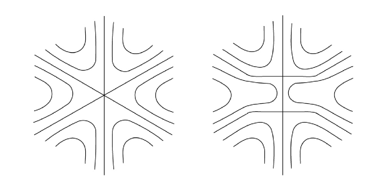
Figure 1. The level sets of $H_{sing}$ (left) and the level sets of $H$ (right) in the case $n=3$.

Lemma 3.2.

Let $s$ be a saddle point of $H$. Then there are coordinates $(x,y)$ about $s$ such that $H=axy$ for $a>0$.

Proof.

First observe that from Remark 3.1 it follows that $H(s)=0$. By Morse lemma, there are coordinates $(x^{\prime},y^{\prime})$ about $s$ such that $H=H(s)-x^{\prime 2}+y^{\prime 2}$. Given $H(s)=0$, we can write

$$H=-x^{\prime 2}+y^{\prime 2}=a\left(\frac{y^{\prime}}{\sqrt{a}}-\frac{x^{\prime}}{\sqrt{a}}\right)\left(\frac{y^{\prime}}{\sqrt{a}}+\frac{x^{\prime}}{\sqrt{a}}\right).$$

Now let

$$x=\frac{y^{\prime}}{\sqrt{a}}+\frac{x^{\prime}}{\sqrt{a}}\quad\mbox{and}\quad y=\frac{y^{\prime}}{\sqrt{a}}-\frac{x^{\prime}}{\sqrt{a}}.$$

Clearly $x$ and $y$ satisfy the statement of the lemma. In addition, the orientation of the pair $(x,y)$ coincides with the orientation of $(x^{\prime},y^{\prime})$. ∎

Let $U_{k}$ be a neighborhood of the $k$-th saddle point $p_{k}$ of $H$ from Lemma 3.2.

3.2. Contact form

Claim 3.3.

If $(M,\omega)$ is an exact symplectic manifold, i.e., $\omega=d\beta$, then the flow $\varphi_{X_{H}}^{t}$ of a Hamiltonian vector field $X_{H}$ consists of exact symplectic maps, i.e.,

$$(\varphi_{X_{H}}^{t})^{\ast}\beta-\beta=df_{t}\quad\mbox{for some function}\ f_{t}.$$

Proof.

Since $\varphi^{0}=id$,

$$(\varphi_{X_{H}}^{t})^{\ast}\beta-\beta=\int\limits^{t}_{0}\frac{d}{ds}(\varphi_{X_{H}}^{s})^{\ast}\beta ds.$$

Since by definition $i_{X_{H}}\omega=-dH$, the integrand is equal to

$$(\varphi_{X_{H}}^{s})^{\ast}L_{X_{H}}\beta =(\varphi^{s})^{\ast}(i_{X_{H}}d\beta+di_{X_{H}}\beta)=(\varphi_{X_{H}}^{s})^{\ast}(-dH+d\beta(X_{H}))$$

$$=d(\varphi_{X_{H}}^{s})^{\ast}(-H+\beta(X_{H}))=d([-H+\beta(X_{H})]\circ\varphi_{X_{H}}^{s}).$$

Thus

$$f_{t}=\int\limits^{t}_{0}(-H+\beta(X_{H}))\circ\varphi_{X_{H}}^{s}ds.$$

∎

Notice that our definition of $X_{H}$ is slightly different from the standard one; usually $X_{H}$ is defined by $i_{X_{H}}\omega=dH$.

Note that the condition that $\beta(X_{H})=H$ is equivalent to the condition that $L_{X_{H}}\beta=0$.

Remark 3.4.

Let $f:=f_{1}=\int^{1}_{0}(-H+\beta(X_{H}))\circ\varphi_{X_{H}}^{s}ds$. In addition, let $S\subset M$ be a region such that $\beta(X_{H})=H$ on $S$ and $S^{\prime}:=\{s\in S:\varphi_{X_{H}}^{t}(s)\in S\ \forall t\in[0,1]\}$. Then $f|_{S^{\prime}}=0$ and $(\varphi^{1}_{X_{H}})^{\ast}(\beta)=\beta$ on $S^{\prime}$.

In the next two lemmas we construct a $1$-form $\beta$ on $\mathbb{R}^{2}$ with $d\beta>0$ and show that $\beta$ is “adapted” to $H$, i.e., $\varphi_{X_{H}}^{\ast}\beta=\beta$ near the saddle points of $H$ and on the region far enough from $D(r_{sing})$, where $X_{H}$ is a Hamiltonian vector field with respect to $d\beta$ and $\varphi_{X_{H}}$ is the time-$1$ map of the flow of $X_{H}$. The condition that $\beta(X_{H})=H$ and Remark 3.4 will play a crucial role when we will compare $\varphi_{X_{H}}^{\ast}\beta$ and $\beta$.

Lemma 3.5.

There exists a 1-form $\beta$ on $\mathbb{R}^{2}$ satisfying the following:

• $d\beta>0$;

• the singular foliation given by $ker(\beta)$ has isolated singularities and no closed orbits;

• the elliptic points of the singular foliation of $\beta$ are the saddle points of $H$; $\beta=\frac{\varepsilon}{2}(xdy-ydx)$ on $U_{k}$ with respect to the coordinates from Lemma 3.2, where $k\in\{1,\dots,n-1\}$ and $\varepsilon$ is a small positive real number;

• $\beta=\frac{1}{2}r^{2}d\theta$ on $\mathbb{R}^{2}\setminus D(r_{sing})$ with respect to the polar coordinates whose origin is at the center of $D(r_{sing})$;

• the hyperbolic points of the singular foliation of $\beta$ are located on $\gamma$, outside of $U_{k}$’s and distributed in such a way that between each two closest elliptic points there is exactly one hyperbolic point.

Proof.

Consider a singular foliation $\mathcal{F}$ on $\mathbb{R}^{2}$ which satisfies the following:

• $\mathcal{F}$ is Morse-Smale and has no closed orbits.

• The singular set of $\mathcal{F}$ consists of elliptic points and hyperbolic points. The elliptic points are the saddle points of $H$. The hyperbolic points are located on $\gamma$ and distributed in such a way that between each two closest elliptic points there is exactly one hyperbolic point. In addition, the hyperbolic points are outside of $U_{k}$’s.

• $\mathcal{F}$ is oriented, and for one choice of orientation the flow is transverse to and exits from $\partial D(r_{sing})$.

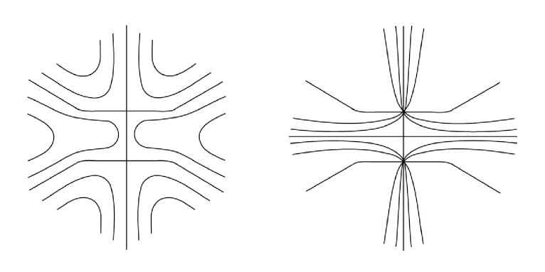
Figure 2. The level sets of $H$ (left) and the characteristic foliation of $\beta$ (right) in the case $n=3$

Next, we modify $\mathcal{F}$ near each of the singular points so that $\mathcal{F}$ is given by $\beta_{0}=\frac{1}{2}(xdy-ydx)$ on $U_{k}$ with respect to the coordinates from Lemma 3.2, and $\beta_{0}=2xdy+ydx$ near a hyperbolic point. In addition, on $\mathbb{R}^{2}\setminus D(r_{sing})$, $\beta_{0}=\frac{1}{2}r^{2}d\theta$ with respect to the polar coordinates whose origin is at the center of $D(r_{sing})$. Finally, we get $\mathcal{F}$ given by $\beta_{0}$, which satisfies $d\beta_{0}>0$ near the singular points and on $\mathbb{R}^{2}\setminus D(r_{sing})$. Now let $\beta=g\beta_{0}$, where $g$ is a positive function with $dg(X)\gg 0$ outside of $(\cup^{n-1}_{k=1}U_{k})\cup(\mathbb{R}^{2}\setminus D(r_{sing}))$, $g|_{\cup^{n-1}_{k=1}U_{k}}=\varepsilon$, $g|_{\mathbb{R}^{2}\setminus D(r_{sing})}=1$ and $X$ is an oriented vector field for $\mathcal{F}$ (nonzero away from the singular points). Since $d\beta=dg\wedge\beta_{0}+g\wedge d\beta_{0}$, $dg(X)\gg 0$ guarantees that $d\beta>0$. Here $\varepsilon$ is a small positive real number. ∎

Remark 3.6.

From the previous lemma we get $\beta$ defined on $\mathbb{R}^{2}$ with the following properties:

• $d\beta>0$ on $\mathbb{R}^{2}$.

• $\beta=\frac{\varepsilon}{2}(xdy-ydx)$ and $H=axy$ on $U_{k}$ for $k=1,\dots,n-1$. In other words, the saddle points of $H$ are exactly the elliptic singularities of $\beta$.

• $\beta=\frac{1}{2}r^{2}d\theta$ and $H=\mu r^{2}\cos(n\theta)$ on $\mathbb{R}^{2}\setminus D(r_{sing})$.

For the comparison of the level sets of $H$ with the singular foliation of $\beta$ in the case $n=3$ we refer to Figure 2.

Lemma 3.7.

Let $\beta$ be a $1$-form from Lemma 3.5. The Hamiltonian vector field $X_{H}$ of $H$ with respect to the area form $d\beta$ satisfies $\beta(X_{H})=H$ on $(\cup_{k=1}^{n-1}U_{k})\cup(\mathbb{R}^{2}\setminus D(r_{sing}))$.

Proof.

First we work on $U_{k}$, where $k\in\{1,\dots,n-1\}$. From Remark 3.6 it follows that $\beta=\frac{\varepsilon}{2}(xdy-ydx)$ and $H=axy$ on $U_{k}$. Let $X_{H}$ be a Hamiltonian vector field defined by $i_{X_{H}}d\beta=-dH$. We show that

$$X_{H}=-\frac{ax}{\varepsilon}\frac{\partial}{\partial x}+\frac{ay}{\varepsilon}\frac{\partial}{\partial y}$$

is a solution of the equation

(3.2.1) $$\beta(X_{H})=H$$

on $U_{k}$. We calculate

$$i_{X_{H}}(d\beta)=(-\frac{ax}{\varepsilon}\frac{\partial}{\partial x}+\frac{ay}{\varepsilon}\frac{\partial}{\partial y})\lrcorner(\varepsilon dx\wedge dy)=-axdy-aydx=-dH$$

and

$$\beta(X_{H})=\frac{\varepsilon}{2}(xdy-ydx)\left(-\frac{ax}{\varepsilon}\frac{\partial}{\partial x}+\frac{ay}{\varepsilon}\frac{\partial}{\partial y}\right)=axy=H.$$

Next, by Remark 3.6, $\beta=\frac{1}{2}r^{2}d\theta$ and $H=\mu r^{2}\cos(n\theta)$ on $\mathbb{R}^{2}\setminus D(r_{sing})$.

As in the previous case, we show that

$$X_{H}=n\mu r\sin(n\theta)\frac{\partial}{\partial r}+2\mu\cos(n\theta)\frac{\partial}{\partial\theta}$$

is a solution of Equation (3.2.1) on $\mathbb{R}^{2}\setminus D(r_{sing})$. We calculate

$$i_{X_{H}}(d\beta) =(n\mu r\sin(n\theta)\partial_{r}+2\mu\cos(n\theta)\partial_{\theta})\lrcorner(rdr\wedge d\theta)$$

$$=-2\mu r\cos(n\theta)dr+n\mu r^{2}\sin(n\theta)d\theta=-dH$$

and

$$\beta(X_{H})=\left(\frac{1}{2}r^{2}d\theta\right)\left(n\mu r\sin(n\theta)\frac{\partial}{\partial r}+2\mu\cos(n\theta)\frac{\partial}{\partial\theta}\right)=\mu r^{2}\cos(n\theta)=H.$$

∎

Let $\varphi^{s}_{X_{H}}$ be the time-$s$ flow of $X_{H}$. Consider

$$S:=\{x\in\mathbb{R}^{2}\setminus D(r_{sing}):\varphi_{X_{H}}^{s}(x)\in\mathbb{R}^{2}\setminus D(r_{sing})\ \forall s\in[0,1]\}\quad\mbox{and}$$

$$V_{k}:=\{x\in U_{k}:\varphi_{X_{H}}^{s}(x)\in U_{k}\ \forall s\in[0,1]\}.$$

Since the saddle points of $H$ are the fixed points of $\varphi^{s}_{X_{H}}$ for $s\in[0,1]$, $V_{k}$ contains an open neighborhood about the $k$-th saddle point of $H$. In addition, note that $S$ contains the level sets of $H$ which do not intersect $D(r_{sing})$, and $(\mathbb{R}^{2}\setminus D(R))$, where $R\gg r_{sing}$. For ease of notation, we write $\varphi_{X_{H}}$ instead of $\varphi^{1}_{X_{H}}$.

Remark 3.8.

Lemma 3.7 implies that $\varphi_{X_{H}}^{\ast}(\beta)=\beta$ on $S\cup(\cup^{n-1}_{k=1}V_{k})$.

Remark 3.9.

From Remark 3.1 and the fact that the flow of $X_{H}$ preserves the level sets of $H$ it follows that $\{p_{k}\}^{n-1}_{k=1}$ is the set of periodic points of $\varphi_{X_{H}}$ on $\mathbb{R}^{2}$.

In the next lemma we construct a contact form $\alpha$ on $D^{2}\times[-1,1]$ such that $R_{\alpha}$ has vertical trajectories.

Lemma 3.10.

Let $\beta_{0}$ and $\beta_{1}$ be two $1$-forms on $D^{2}$ such that $\beta_{0}=\beta_{1}$ in a neighborhood of $\partial D^{2}$ and $d\beta_{0}=d\beta_{1}=\omega>0.$ Then there exists a contact $1$-form $\alpha$ with Reeb vector field $R_{\alpha}$ on $[-1,1]\times D^{2}$ with coordinates $(t,x)$, where t is a coordinate on $[-1,1]$ and $x$ is a coordinate on $D^{2}$, with the following properties:

• $\alpha=dt+\varepsilon\beta_{0}$ in a neighborhood of $\{-1\}\times D^{2}$;

• $\alpha=dt+\varepsilon\beta_{1}$ in a neighborhood of $\{1\}\times D^{2}$;

• $R_{\alpha}$ is collinear to $\frac{\partial}{\partial t}$ on $[-1,1]\times D^{2}$;

• $R_{\alpha}=\frac{\partial}{\partial t}$ in a neighborhood of $[-1,1]\times\partial D^{2}$.

Here $\varepsilon$ is a small positive number.

Proof.

Since $D^{2}$ is simply connected and $\omega=d\beta_{0}=d\beta_{1}>0$, there exists a function $h\in C^{\infty}(D^{2})$ such that $\beta_{1}-\beta_{0}=dh$. Let $\chi_{0}\colon\thinspace[-1,1]\to[0,1]$ be a smooth map for which $\chi_{0}(t)=0$ for $-1\leq t\leq-1+\varepsilon_{\chi_{0}}$, $\chi_{0}(t)=1$ for $1-\varepsilon_{\chi_{0}}\leq t\leq 1$ and $\chi_{0}^{\prime}(t)\geq 0$ for $t\in[-1,1]$, where $\varepsilon_{\chi_{0}}$ is a small positive number. In addition, we define $\chi_{1}(t):=\chi_{0}^{\prime}(t)$.

Consider $[-1,1]\times D^{2}$ equipped with a $1$-form

$$\alpha=(1+\varepsilon\chi_{1}(t)h)dt+\varepsilon((1-\chi_{0}(t))\beta_{0}+\chi_{0}(t)\beta_{1}).$$

We then compute

$$d\alpha =\varepsilon(\chi_{1}(t)dh\wedge dt+(1-\chi_{0}(t))d\beta_{0}+\chi_{0}(t)d\beta_{1}+\chi_{0}^{\prime}(t)dt\wedge\beta_{1}-\chi_{0}^{\prime}(t)dt\wedge\beta_{0})$$

$$=\varepsilon(\chi_{1}(t)dh\wedge dt+\chi_{0}^{\prime}(t)dt\wedge\beta_{1}-\chi_{0}^{\prime}(t)dt\wedge\beta_{0})+\varepsilon\omega$$

$$=\varepsilon(\chi_{1}(t)dh\wedge dt-\chi_{0}^{\prime}(t)\beta_{1}\wedge dt+\chi_{0}^{\prime}(t)\beta_{0}\wedge dt)+\varepsilon\omega$$

$$=\varepsilon(\chi_{1}(t)dh\wedge dt-\chi_{0}^{\prime}(t)(\beta_{1}-\beta_{0})\wedge dt)+\varepsilon\omega$$

$$=\varepsilon(\chi_{1}(t)dh\wedge dt-\chi_{0}^{\prime}(t)dh\wedge dt)+\varepsilon\omega$$

$$=\varepsilon(\chi_{1}(t)-\chi_{0}^{\prime}(t))dh\wedge dt+\varepsilon\omega=\varepsilon\omega$$

and hence

$$\alpha\wedge d\alpha =((1+\varepsilon\chi_{1}(t)h)dt+\varepsilon((1-\chi_{0}(t))\beta_{0}+\chi_{0}(t)\beta_{1}))\wedge\varepsilon\omega$$

$$=\varepsilon dt\wedge\omega+\varepsilon^{2}(\chi_{1}(t)hdt+(1-\chi_{0}(t))\beta_{0}+\chi_{0}(t)\beta_{1})\wedge\omega.$$

If $\varepsilon$ is sufficiently small, then $\alpha$ satisfies the contact condition, i.e., $\alpha\wedge d\alpha>0$.

Now let us show that the Reeb vector field $R_{\alpha}$ is given by

$$R_{\alpha}=\frac{1}{1+\varepsilon\chi_{1}(t)h}\frac{\partial}{\partial t}.$$

First we compute

$$i_{R_{\alpha}}(d\alpha) =\left(\frac{1}{1+\varepsilon\chi_{1}(t)h}\partial_{t}\right)\lrcorner(\varepsilon\omega)=0.$$

Then we check the normalization condition, i.e., $\alpha(R_{\alpha})=1$:

$$\alpha(R_{\alpha}) =((1+\varepsilon\chi_{1}(t)h)dt+\varepsilon((1-\chi_{0}(t))\beta_{0}+\chi_{0}(t)\beta_{1}))\left(\frac{1}{1+\varepsilon\chi_{1}(t)h}\frac{\partial}{\partial t}\right)$$

$$=\frac{1+\varepsilon\chi_{1}(t)h}{1+\varepsilon\chi_{1}(t)h}=1.$$

Since $\beta_{1}=\beta_{0}$ in a neighborhood of $\partial D$, $h=0$ in a neighborhood of $\partial D^{2}$ and hence $R_{\alpha}=\frac{\partial}{\partial t}$ in a neighborhood of $[-1,1]\times\partial D^{2}$. Finally, we see that $\alpha$ satisfies Conditions $(1)-(4)$. ∎

Fix $R_{\ast}\gg r_{sing}$ such that there is an annular neighborhood $V_{R_{\ast}}$ of $\partial D(R_{\ast})$ in $\mathbb{R}^{2}$ with $V_{R_{\ast}}\subset S$. Consider $D(R_{\ast})$ with two $1$-forms $\beta_{0}:=\beta|_{D(R_{\ast})}$, where $\beta$ is a $1$-form from Lemma 3.5, and $\beta_{1}:=\varphi_{X_{H}}^{\ast}(\beta)|_{D(R_{\ast})}$. By Remark 3.8,

(3.2.2) $$\beta_{0}=\beta_{1}\quad\mbox{on}\quad V_{R_{\ast}}\cap D(R_{\ast}).$$

In addition, we have

(3.2.3) $$d\beta_{1}=d(\varphi_{X_{H}}^{\ast}(\beta)|_{D(R_{\ast})})=\varphi_{X_{H}}^{\ast}(d\beta)|_{D(R_{\ast})}=(d\beta)|_{D(R_{\ast})}=d\beta_{0}>0.$$

From Equations (3.2.2) and (3.2.3) it follows that $\beta_{0}$ and $\beta_{1}$ satisfy the conditions of Lemma 3.10.

Now take $[-1,1]\times D(R_{\ast})$ with the contact $1$-form $\alpha$ from Lemma 3.10 with $\beta_{0}$ and $\beta_{1}$ as in the previous paragraph. Note that $\beta_{1}-\beta_{0}=dh$ for $h\in C^{\infty}(D(R_{\ast}))$. We can rewrite this equation as

(3.2.4) $$\varphi_{X_{H}}^{\ast}(\beta)|_{D(R_{\ast})}-\beta|_{D(R_{\ast})}=dh.$$

Let us remind that

$$\varphi_{X_{H}}^{\ast}(\beta)-\beta=df$$

on $\mathbb{R}^{2}$, where

$$f=\int^{1}_{0}(-H+\beta(X_{H}))\circ\varphi_{X_{H}}^{s}ds.$$

Hence, $h:=f|_{D(R_{\ast})}$ satisfies Equation (3.2.4). From Remark 3.4 it follows that $f|_{D(R_{\ast})}=0$ on $(\cup^{n-1}_{k=1}V_{k})\cup(D(R_{\ast})\cap S)$. Thus, $h=0$ on $(\cup^{n-1}_{k=1}V_{k})\cup(D(R_{\ast})\cap S)$.

Remark 3.11.

Since $h=0$ on $(\cup^{n-1}_{k=1}V_{k})\cup(D(R_{\ast})\cap S)$, by the construction of $\alpha$, $R_{\alpha}=\partial_{t}$ on $(\cup^{n-1}_{k=1}[-1,1]\times V_{k})\cup([-1,1]\times(D(R_{\ast})\cap S))$.

Let $\beta_{-}:=\varepsilon\beta_{0}$ and $\beta_{+}:=\varepsilon\beta_{1}$, where $\varepsilon$ is a constant from Lemma 3.10 which makes $\alpha$ contact.

3.3. Gluing

In this section we will construct the sutured contact solid torus with $2n$ parallel longitudinal sutures, where $n\geq 2$.

First we construct surfaces with boundary $P_{+},P_{-},D\subset\mathbb{R}^{2}$ with the following properties:

• $P_{\pm}\subset D$;

• $(\partial P_{\pm})_{\partial}\subset\partial D$ and $(\partial P_{\pm})_{int}\subset int(D)$;

• $\varphi_{X_{H}}$ maps $P_{+}$ to $P_{-}$ in such a way that $\varphi_{X_{H}}((\partial P_{+})_{int})=(\partial P_{-})_{\partial}$ and $\varphi_{X_{H}}((\partial P_{+})_{\partial})=(\partial P_{-})_{int}$;

• $(\partial P_{-})_{\partial}\cap(\partial P_{+})_{\partial}=\emptyset$.

Recall that

$$X_{H}=n\mu r\sin(n\theta)\frac{\partial}{\partial r}+2\mu\cos(n\theta)\frac{\partial}{\partial\theta}\quad\mbox{and}\quad\beta_{-}=\beta_{+}=\frac{\varepsilon}{2}r^{2}d\theta$$

on $D(R_{\ast})\cap S$. Note that $X_{H}$ is collinear to $-\partial_{r}$ for $\theta=\frac{3\pi}{2n}+\frac{2\pi k}{n}$, where $k\in\{0,\dots,n-1\}$. For simplicity, let us denote

$$\theta^{-}_{k}:=\frac{3\pi}{2n}+\frac{2\pi k}{n}-\frac{\pi}{2n}\quad\mbox{and}\quad\theta^{+}_{k}:=\frac{3\pi}{2n}+\frac{2\pi k}{n}+\frac{\pi}{2n},$$

where $k\in\{0,\dots,n-1\}$.

Fix $R$ such that $r_{sing}\ll R\ll R_{\ast}$ and there is an annular neighborhood $V(R)$ of $\partial D(R)$ in $D(R_{\ast})$ satisfying $\{(r,\theta)\ :\ R\leq r\leq R_{\ast}\}\subset V(R)\subset S\cap D(R_{\ast})$.

Consider $D(R)\subset D(R_{\ast})$. Let $a^{+}_{k}$ be a segment on $\partial D(R)$ which starts at $(R,\theta^{-}_{k})$ and ends at $(R,\theta^{+}_{k})$, i.e., $a^{+}_{k}:=\{(R,\theta):\theta^{-}_{k}\leq\theta\leq\theta^{+}_{k}\}$.

Consider $\cup_{k=0}^{n-1}\varphi_{X_{H}}(a^{+}_{k})$. It is easy to see that every level set of $H$ which intersects $a^{+}_{k}$ intersects it only once. Hence, using that there are no closed level sets of $H$ and $X_{H}$ is $\frac{2\pi}{n}$-symmetric on $D(R_{\ast})\setminus D(r_{sing})$, we get

$$\left(\bigcup_{k=0}^{n-1}\varphi_{X_{H}}(a^{+}_{k})\right)\bigcap\left(\bigcup_{k=0}^{n-1}a^{+}_{k}\right)=\emptyset.$$

Let $a^{-}_{k}:=\varphi_{X_{H}}(a^{+}_{k})$. By possibly making $R$ and $R_{\ast}$ big enough, we can make $a^{-}_{k}$’s to be in $V(R)$. Consider the endpoints of $a^{-}_{k}$’s. Since $X_{H}$ is $\frac{2\pi}{n}$-symmetric outside of $D(r_{sing})$, it is easy to see that $\varphi_{X_{H}}(R,\theta^{-}_{k})=(\tilde{R},\tilde{\theta}^{-}_{k})$ and $\varphi_{X_{H}}(R,\theta^{+}_{k})=(\tilde{R},\tilde{\theta}^{+}_{k})$, where $\theta^{-}_{k}-\frac{\pi}{2n}<\tilde{\theta}^{-}_{k}<\theta^{-}_{k}$, $\theta^{+}_{k}<\tilde{\theta}^{+}_{k}<\theta^{+}_{k}+\frac{\pi}{2n}$ and $\tilde{R}>R$. In addition, observe that $\tilde{R}$ is the same for all endpoints of $a^{+}_{k}$’s.

Let $\{b^{+}_{k}\}_{k=0}^{n-1}$ be a set of embedded curves on $D(R_{\ast})$ with the following properties:

• $b^{+}_{k-1}$ starts at the terminal point of $a^{+}_{k-1}$ and ends at the initial point of $a^{+}_{k}$, where $k$ is considered mod $n$;

• $b^{+}_{k-1}\subset\{(r,\theta):r>r_{sing},\ \theta^{+}_{k-1}\leq\theta\leq\theta^{-}_{k}\}$ and $b^{+}_{k-1}\subset V(R)$ for $k=0,\dots,n-1$;

• $\varphi_{X_{H}}(b^{+}_{k})\subset\{(r,\theta):r>R\}\subset V(R)$ for $k=0,\dots,n-1$;

• the region bounded by $a^{+}_{k}$’s and $b^{+}_{k}$’s has smooth boundary;

• each level set of $H$ which intersects $b^{+}_{k}$ intersects it only once.

For simplicity, we take $\frac{2\pi}{n}$-symmetric $b^{+}_{k}$’s, i.e., $b^{+}_{k+1}$ can be obtained from $b^{+}_{k}$, where $k$ is considered mod $n$, by doing $\frac{2\pi}{n}$-positive rotation about the center of $D(R_{\ast})$.

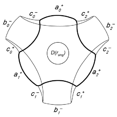
Figure 3. Construction of $P_{+}$, $P_{-}$ and $D$ in the case $n=3$

Note that Properties $(P_{2})$ and $(P_{3})$ and the form of $X_{H}$ on $D(R_{\ast})\setminus D(r_{sing})$ imply that

(3.3.1) $$\varphi_{X_{H}}(b^{+}_{k-1})\subset\{(r,\theta)\ :\ r>R,\ \tilde{\theta}^{+}_{k-1}\leq\theta\leq\tilde{\theta}^{-}_{k}\}\subset V(R),$$

where $k\in\{0,\dots,n-1\}$. Again, using that the level sets of $H$ which intersects $b^{+}_{k}$ intersects it only once, there are no closed level sets of $H$ and $X_{H}$ is $\frac{2\pi}{n}$-symmetric, we obtain

$$\left(\bigcup_{k=0}^{n-1}\varphi_{X_{H}}(b^{+}_{k})\right)\bigcap\left(\bigcup_{k=0}^{n-1}b^{+}_{k}\right)=\emptyset.$$

Let $b^{-}_{k}:=\varphi_{X_{H}}(b^{+}_{k})$. From Formula (3.3.1) and the construction of $a^{+}_{k}$’s it follows that

(3.3.2) $$\left(\bigcup_{k=0}^{n-1}a^{+}_{k}\right)\bigcap\left(\bigcup_{k=0}^{n-1}b^{-}_{k}\right)=\emptyset.$$

Then we connect the terminal point of $a^{+}_{k}$ with the initial point of $b^{-}_{k}$ by the line segment $c^{-}_{k}$ and the terminal point of $b^{-}_{k}$ with the initial point of $a^{+}_{k+1}$ by the line segment $c^{+}_{k}$. From the construction above it follows that $c^{-}_{k}$ intersects $D(R)$ only at the terminal point of $a^{+}_{k}$, and $c^{+}_{k}$ intersects $D(R)$ only at the initial point of $a^{+}_{k+1}$. Then we round the corners between $c^{-}_{k}$ and $a^{+}_{k}$, $c^{-}_{k}$ and $b^{-}_{k}$, $c^{+}_{k}$ and $b^{-}_{k}$, $c^{+}_{k}$ and $a^{+}_{k+1}$. Finally, we get a surface whose boundary consists of $a^{+}_{k}$’s, $b^{-}_{k}$’s, $c^{+}_{k}$’s and $c^{-}_{k}$’s, which we call $D$. See Figure 3.

Remark 3.12.

By the construction, $a^{\pm}_{k}$’s, $b^{\pm}_{k}$’s and $c^{\pm}_{k}$ lie in $V(R)\subset D(R_{\ast})\cap S$.

Now we take $[-1,1]\times D$ with a contact form $\alpha:=\alpha|_{[-1,1]\times D}$ and contact structure $\xi=ker(\alpha)$. Let $\Gamma=\{0\}\times\partial D$ in $[-1,1]\times D$ and $U(\Gamma):=[-1,0]\times[-1,1]\times\Gamma$ be a neighborhood of $\Gamma$ with coordinates $(\tau,t)\in[-1,0]\times[-1,1]$, where $t$ is a usual $t$-coordinate on $[-1,1]\times D$. By Remark 3.12, we can make $U(\Gamma)$ such that

(3.3.3) $$U(\Gamma)\subset[-1,1]\times(D\cap S).$$

Observe that $\partial_{h}([-1,1]\times D)=R_{+}\cup R_{-}$, where $R_{+}=\{-1\}\times D$ and $R_{+}=\{1\}\times D$ with respect to the coordinates on $[-1,1]\times D$. In addition, $\partial_{v}([-1,1]\times D)=[-1,1]\times\partial D$ with respect the coordinates on $[-1,1]\times D$. Let $\beta_{\pm}:=\beta_{\pm}|_{\{\pm 1\}\times D}$.

Lemma 3.13.

$([-1,1]\times D,\Gamma,U(\Gamma),\xi)$ is a sutured contact manifold and $\alpha$ is an adapted contact form.

Proof.

First note that $\alpha|_{R{-}}=\beta_{-}$ and $\alpha|_{R_{+}}=\beta_{+}$. Let us check that $(R_{-},\beta_{-})$ and $(R_{+},\beta_{+})$ are Liouville manifolds. From the construction of $\beta_{\pm}$ it follows that $d(\beta_{-})=d(\beta_{+})>0$. Since $\beta_{-}=\beta_{+}$ on $D\cap S$, by Equation (3.3.3), we have $\alpha=dt+\beta_{-}$ on $U(\Gamma)$. Recall that $\beta_{-}=\beta_{+}=\frac{\varepsilon}{2}r^{2}d\theta$ on $D\cap S$. Hence, $\alpha|_{U(\Gamma)}=dt+\frac{\varepsilon}{2}r^{2}d\theta$. The calculation

$$i_{Y_{\pm}|_{R_{\pm}\cap U(\Gamma)}}(d\beta_{\pm})=\left(\frac{1}{2}r\partial_{r}\right)\lrcorner(\varepsilon rdr\wedge d\theta)=\frac{\varepsilon}{2}r^{2}d\theta=\beta_{\pm}$$

implies that the Liouville vector fields $Y_{\pm}|_{R_{\pm}\cap U(\Gamma)}$ are equal to $\frac{1}{2}r\partial_{r}$. From the construction of $D$ it follows that $Y_{\pm}$ is positively transverse to $\partial R_{\pm}$. Therefore, $(R_{-},\varepsilon\beta_{0})$ and $(R_{+},\varepsilon\beta_{1})$ are Liouville manifolds. As we already mentioned, $\alpha=dt+\beta_{-}$ on $U(\Gamma)$. Finally, if we take $\tau$ such that $\partial_{\tau}=\frac{1}{2}r\partial_{r}$, then $([-1,1]\times D,\Gamma,U(\Gamma),\xi)$ becomes a sutured contact manifold with an adapted contact form $\alpha$. ∎

Now observe that from the construction of $\alpha$ it follows that $\alpha|_{[-1,-1+\varepsilon_{\chi_{0}}]\times D}=dt+\beta_{-}$ and $\alpha|_{[1-\varepsilon_{\chi_{0}},1]\times D}=dt+\beta_{+}$. Then we define $P_{\pm}\subset R_{\pm}$. Let $P_{+}$ be a region bounded by $a^{+}_{k}$’s and $b^{+}_{k}$’s in $R_{+}$ and let $P_{-}$ be a region bounded by $a^{-}_{k}$’s and $b^{-}_{k}$’s in $R_{-}$. Note that from Remark 3.12 it follows that $a^{\pm}_{k}$’s and $b^{\pm}_{k}$ are in $S$. Hence, by Lemma 3.13, $Y_{\pm}=\frac{1}{2}r\partial_{r}$ along $\partial P_{\pm}$. The construction of $a^{\pm}_{k}$’s and $b^{\pm}_{k}$ implies that $Y_{\pm}$ is positively transverse to $\partial P_{\pm}$. From the construction we made it is easy to see that $(\partial P_{+})_{\partial}=\cup_{k=0}^{n-1}a^{+}_{k}$, $(\partial P_{+})_{int}=\cup_{k=0}^{n-1}b^{+}_{k}$, $(\partial P_{-})_{\partial}=\cup_{k=0}^{n-1}b^{-}_{k}$ and $(\partial P_{-})_{int}=\cup_{k=0}^{n-1}a^{-}_{k}$. If $\pi\colon\thinspace[-1,1]\times D\to D$ is a projection to $D$ along $\partial_{t}$, then from Equation (3.3.2) it follows that $\pi((\partial P_{-})_{\partial})\cap\pi((\partial P_{+})_{\partial})=\emptyset$. Observe that $\varphi_{X_{H}}^{\ast}(\beta_{-}|_{P_{-}})=\beta_{+}|_{P_{+}}$ and $\varphi_{X_{H}}(a^{+}_{k})=a^{-}_{k}$, $\varphi_{X_{H}}(b^{+}_{k})=b^{-}_{k}$ for $k=0,\dots,n-1$. Hence, by definition of $P_{\pm}$, $\varphi_{X_{H}}$ sends $P_{+}$ to $P_{-}$ in such a way that $(\partial P_{+})_{int}$ maps to $(\partial P_{-})_{\partial}$ and $(\partial P_{+})_{\partial}$ maps to $(\partial P_{-})_{int}$.

Next, we follow the gluing procedure overviewed in Section 2.7 and completely described in [3]. We get a sutured contact manifold $(S^{1}\times D^{2},\tilde{\Gamma},U(\tilde{\Gamma}),\tilde{\alpha})$. For simplicity, we omit index $N$. Observe that the region enclosed by $\partial D$ and $a^{-}_{k}$ in $D\setminus P_{-}$ contains $a^{+}_{k}$ and the region enclosed by $\partial D$ and $b^{+}_{k}$ in $D\setminus P_{+}$ contains $b^{-}_{k}$. Then from the gluing construction and the form of $\varphi_{X_{H}}$ near the boundary of $P_{+}$ it follows that $\tilde{\Gamma}$ has $2n$ parallel longitudinal components.

3.4. Reeb orbits

Consider $(S^{1}\times D^{2},\tilde{\Gamma},U(\tilde{\Gamma}),\tilde{\alpha})$ obtained in Section 3.3. Recall that $\tilde{\Gamma}$ consists of $2n$ parallel longitudinal curves. Let $\tilde{\xi}$ denote the contact structure defined by $\tilde{\alpha}$ and $R_{\tilde{\alpha}}$ denote the Reeb vector field defined by $\tilde{\alpha}$. The main goal of this section is to understand the set of embedded, closed orbits of $R_{\tilde{\alpha}}$.

Definition 3.14.

Let $S$ be a non-empty set with two non-empty subsets $S_{1}$ and $S_{2}$ such that $S_{1}\cap S_{2}\neq\emptyset$, and let $f\colon\thinspace S_{1}\to S_{2}$. A point $s\in S_{1}$ is called a periodic point of $f$ of period $n$ if $f^{n}(s)$ is well-defined, i.e., $f^{i}(s)\in S_{1}\cap S_{2}$ for $i=1,\dots,n-1$, and $f^{n}(s)=s$.

Lemma 3.15.

$R_{\tilde{\alpha}}$ has $n-1$ embedded, closed orbits.

Proof.

First consider $\varphi_{X_{H}}|_{P_{+}}$. Recall that from the construction of $P_{-}$ and $P_{+}$ it follows that $\varphi_{X_{H}}(P_{+})=P_{-}$. Hence, by Remark 3.9, $\{p_{k}\}^{n-1}_{k=1}$ is the set of periodic points of $\varphi_{X_{H}}|_{P_{+}}$.

From the construction of $\alpha$ on $[-1,1]\times D$ and the gluing construction it follows that there is a one-to-one correspondence between the set of embedded Reeb orbits and the set of periodic points of $\varphi_{X_{H}}|_{P_{+}}$. Thus, there are $n-1$ embedded closed orbits of $R_{\tilde{\alpha}}$. ∎

Let $\gamma_{k}$ be the embedded, closed orbit, which corresponds to the periodic point $p_{k}$, i.e., $\gamma_{k}$ is obtained from $[-1,1]\times\{p_{k}\}\subset[-1,1]\times D$.

Lemma 3.16.

$\gamma^{s}_{k}$ is a nondegenerate orbit for $k\in\{1,\dots,n-1\}$ and $s\in\mathbb{N}$. Moreover $\{\gamma_{k}\}^{n-1}_{k=1}$ is a set of positive hyperbolic orbits and $\int\limits_{\gamma_{l}}\tilde{\alpha}=\int\limits_{\gamma_{m}}\tilde{\alpha}$ for $l,m=1,\dots,n-1$.

Proof.

Let

$$M^{(0)}=(([-1,1]\times D)\cup(R_{+}(\Gamma)\times[1;\infty))\cup(R_{+}(\Gamma)\times(-\infty;-1]))$$

and

$$\tilde{M}=M^{(0)}\setminus((P_{+}\times(N,\infty)\cup(P_{-}\times(-\infty,-N)).$$

In addition, let $\alpha_{\tilde{M}}$ denote the contact form on $\tilde{M}$ and let $\xi_{\tilde{M}}$ denote the contact structure defined by $\alpha_{\tilde{M}}$.

Consider $[-1,1]\times D\subset\tilde{M}$. From the construction of $\alpha$ it follows that $\alpha|_{[-1,1]\times V_{k}}=dt+\beta_{-}$. Since the contact structure on $[1,\infty)\times P_{+}$ is given by $dt+\beta_{+}$ and the contact structure on $(-\infty,-1]\times P_{-}$ is given by $dt+\beta_{-}$, $\alpha_{\tilde{M}}|_{[-N,N]\times V_{k}}=dt+\beta_{-}$ on $[-N,N]\times V_{k}\subset\tilde{M}$. Therefore, we get

(3.4.1) $$\int\limits_{[-N,N]\times\{p_{k}\}}\alpha_{\tilde{M}}=2N.$$

From the gluing construction and Equation (3.4.1) it follows that $\int_{\gamma_{k}}\tilde{\alpha}=2N$. Note that $\int_{\gamma_{k}}\tilde{\alpha}$ does not depend on $k$. Hence, $\int_{\gamma_{l}}\tilde{\alpha}=\int_{\gamma_{m}}\tilde{\alpha}$ for $l,m=1,\dots,n-1$.

Now observe that $H|_{V_{k}}=axy$ and hence

$$\varphi_{X_{H}}|_{V_{k}}=\left(\begin{array}[]{ll}\lambda&0\\ 0&\lambda^{-1}\end{array}\right),$$

where $\lambda=e^{a}$. Let the symplectic trivialization of $\xi_{\tilde{M}}$ along $[-N,N]\times\{p_{k}\}$ be given by the framing $(\lambda^{\frac{-N-t}{2N}}\partial_{x},\lambda^{\frac{t+N}{2N}}\partial_{y})$. Note that the symplectic trivialization of $\xi_{\tilde{M}}$ gives rise to the symplectic trivialization of $\tilde{\xi}$ along $\gamma_{k}$.

It is easy to see that the linearized return map $P_{\gamma_{k}}$ is given by

$$P_{\gamma_{k}}=\left(\begin{array}[]{ll}\lambda&0\\ 0&\lambda^{-1}\end{array}\right).$$

Since the eigenvalues of $P_{\gamma_{k}}$ are positive real numbers different from $1$, $\gamma_{k}$ is a positive hyperbolic orbit. Hence, $\{\gamma_{k}\}^{n-1}_{k=1}$ is a set of positive hyperbolic orbits of $R_{\tilde{\alpha}}$. In addition, $P_{\gamma^{s}_{k}}=P^{s}_{\gamma_{k}}$. Therefore, the eigenvalues of $P_{\gamma^{s}_{k}}$ are different from $1$. Hence, $\gamma^{s}_{k}$ is a nondegenerate orbit for $s\in\mathbb{N}$.

∎

4. Calculations

In this section we will calculate the sutured embedded contact homology, the sutured cylindrical contact homology and the sutured contact homology of the sutured contact solid torus constructed in Section 3.3.

Consider the symplectization $(\mathbb{R}\times(S^{1}\times D^{2})^{\ast},d(e^{s}\tilde{\alpha}^{\ast}))$ of $((S^{1}\times D^{2})^{\ast},\tilde{\alpha}^{\ast})$, where $s$ is the coordinate on $\mathbb{R}$ and $((S^{1}\times D^{2})^{\ast},\tilde{\alpha}^{\ast})$ is the completion of $(S^{1}\times D^{2},\tilde{\Gamma},U(\tilde{\Gamma}),\tilde{\alpha})$. Let $J$ be an almost complex structure on $(\mathbb{R}\times(S^{1}\times D^{2})^{\ast},d(e^{s}\tilde{\alpha}^{\ast}))$ tailored to $((S^{1}\times D^{2})^{\ast},\tilde{\alpha}^{\ast})$.

4.1. Sutured embedded contact homology

Consider the set of embedded, closed orbits of $R_{\tilde{\alpha}}$. By Lemma 3.15, $R_{\tilde{\alpha}}$ has $n-1$ embedded, closed orbits $\gamma_{1},\dots,\gamma_{n-1}$, which are positive hyperbolic by Lemma 3.16. In addition, Lemma 3.16 implies that all Reeb orbits are nondegenerate. From the gluing construction, i.e., since $\{p\}^{n-1}_{k=1}$ is a set of fixed points of $\varphi_{X_{H}}$, it follows that $[\gamma_{i}]$ is a generator of $H_{1}(S^{1}\times D^{2};\mathbb{Z})$ for $i\in\{1,\dots,n-1\}$ and $[\gamma_{i}]=[\gamma_{j}]$ for $i,j\in\{1,\dots,n-1\}$. From now on we identify $H_{1}(S^{1}\times D^{2};\mathbb{Z})$ with $\mathbb{Z}$ in such a way that $[\gamma_{i}]\in H_{1}(S^{1}\times D^{2};\mathbb{Z})$ is identified with $1\in\mathbb{Z}$ for $i\in\{1,\dots,n-1\}$. Recall that multiplicities of hyperbolic orbits in an admissible orbit set must be equal to $1$. Hence, from Lemma 3.16 it follows that the admissible orbit sets are of the form $\{(\gamma_{i_{1}},1),\dots,(\gamma_{i_{s}},1)\}$, where $1\leq i_{1}<\dots<i_{s}\leq n-1$. Note that $\emptyset$ is an admissible orbit set. For ease of notation, we write $\gamma_{i_{1}}\dots\gamma_{i_{s}}$ instead of $\{(\gamma_{i_{1}},1),\dots,(\gamma_{i_{s}},1)\}$ and $1$ instead of $\emptyset$, where $1\leq i_{1}<\dots<i_{s}\leq n-1$.

Lemma 4.1.

Let $\partial$ be the ECH differential. Then $\partial(a)=0$ for every admissible orbit set $a$.

Proof.

Fix $h\in H_{1}(S^{1}\times D^{2};\mathbb{Z})$. Let $S_{h}$ be a set of admissible orbit sets with homology class $h$. It is easy to see that

$$S_{h}=\left\{\begin{array}[]{ll}\{\gamma_{i_{1}}\dots\gamma_{i_{h}}\},&\mbox{for}\ 0\leq h\leq n-1;\\ \emptyset,&\mbox{otherwise}.\end{array}\right.$$

From Lemma 3.16 it follows that for every $a\in S_{h}$, $\mathcal{A}(a)=2Nh$. Let $a,b\in S_{h}$ be different admissible orbit sets. Then, as we already mentioned,

(4.1.1) $$\mathcal{A}(a)=\mathcal{A}(b)=2Nh.$$

From Equation (4.1.1) and the second part of Lemma 2.13 it follows that $M^{J}(a,b)$ is empty. In addition, by the second part of Lemma 2.13, every element in $M^{J}(a,a)$ maps to a union of trivial cylinders. Hence, by Proposition 2.15 and definition of $\partial$, $\partial(a)=0$. Note that trivial cylinders are regular and hence we can omit the genericity assumption in Proposition 2.15. Thus, for every admissible orbit set $a$, $\partial(a)=0$. ∎

Again, let $S_{h}$ be a set of admissible orbit sets with homology class $h$.

By counting the number of element in $S_{h}$, we get

(4.1.4) $$|S_{h}|=\left\{\begin{array}[]{ll}{n-1\choose h},&\mbox{for}\ 0\leq h\leq n-1;\\ 0,&\mbox{otherwise}.\end{array}\right.$$

By Equation (4.1.4) and Lemma 4.1, we get

$$ECH(S^{1}\times D^{2},\tilde{\Gamma},\tilde{\alpha},J,h)\simeq\Lambda^{\ast}\langle\gamma_{1},\dots,\gamma_{n-1}\rangle\simeq\left\{\begin{array}[]{ll}\mathbb{Z}^{n-1\choose h},&\mbox{for}\ 0\leq h\leq n-1;\\ 0,&\mbox{otherwise}.\end{array}\right.$$

Here $\Lambda^{\ast}\langle\gamma_{1},\dots,\gamma_{n-1}\rangle$ is the exterior algebra over $\mathbb{Z}$ generated by $\gamma_{1},\dots,\gamma_{n-1}$. Thus, we obtain

$$ECH(S^{1}\times D^{2},\tilde{\Gamma},\tilde{\alpha},J)=\bigoplus\limits_{h\in H_{1}(S^{1}\times D^{2};\mathbb{Z})}ECH(S^{1}\times D^{2},\tilde{\Gamma},\tilde{\alpha},J,h)\simeq\mathbb{Z}^{\sum\limits_{h=0}^{n-1}{n-1\choose h}}=\mathbb{Z}^{2^{n-1}}.$$

This completes the proof of Theorem 1.2.

Remark 4.2.

Note that for the constructed sutured contact solid torus, the sutured Floer homology coincides with the sutured embedded contact homology. In fact, they agree in each Spin^c-structure. This follows from Proposition 9.2 in [15], where the sutured Floer homology of every sutured manifold $(S^{1}\times D^{2},\Gamma)$ has been computed by Juhász.

4.2. Sutured cylindrical contact homology

First recall that Lemma 3.15 implies that all closed orbits of $R_{\tilde{\alpha}}$ are nondegenerate.

Remark 4.3.

Note that there are no contractible Reeb orbits. Hence, from Fact 2.21, Remark 2.24 and the fact that $\pi_{1}(S^{1}\times D^{2};\mathbb{Z})\simeq H_{1}(S^{1}\times D^{2};\mathbb{Z})\simeq\mathbb{Z}$ it follows that for all $h\in H_{1}(S^{1}\times D^{2};\mathbb{Z})$ $HC^{cyl,h}_{\ast}(S^{1}\times D^{2},\tilde{\Gamma},\tilde{\alpha}_{\delta},J)$ is defined, i.e., $\partial^{2}=0$, and is independent of contact form $\tilde{\alpha}$ for the given contact structure $\tilde{\xi}$ and the almost complex structure $J$.

Note that $C_{\ast}(\tilde{\alpha},J)$ splits as

$$C_{\ast}(\tilde{\alpha},J)=\bigoplus\limits_{h\in H_{1}(S^{1}\times D^{2};\mathbb{Z})}C_{\ast}^{h}(\tilde{\alpha},J).$$

From Lemma 3.16 it follows that $\{\gamma_{k}\}^{n-1}_{k=1}$ is a set of positive hyperbolic orbits. Hence, the definition of the Conley-Zehnder index implies that $\mu_{\tau}(\gamma^{s}_{l})$ is even for $l\in\{1,\dots,n-1\}$ and $s\in\mathbb{N}$. Then, according to the definition of a good orbit, it follows that $\gamma^{s}_{l}$ is a good orbit for $l\in\{1,\dots,n-1\}$ and $s\in\mathbb{N}$. Hence, we get

(4.2.1) $$C_{\ast}^{h}(\tilde{\alpha},J)=\left\{\begin{array}[]{ll}\mathbb{Q}\langle\gamma_{1}^{h},\dots,\gamma_{n-1}^{h}\rangle,&\mbox{for}\ h\geq 1;\\ 0,&\mbox{otherwise}.\end{array}\right.$$

Here $\mathbb{Q}\langle\gamma_{1}^{h},\dots,\gamma_{n-1}^{h}\rangle$ is a $\mathbb{Q}$-module freely generated by $\gamma_{1}^{h},\dots,\gamma_{n-1}^{h}$. Now recall that Lemma 3.16 says that $\int_{\gamma_{l}}\tilde{\alpha}=\int_{\gamma_{m}}\tilde{\alpha}=2N$, where $l,m\in\{1,\dots,n-1\}$. Therefore,

(4.2.2) $$\int\limits_{\gamma^{s}_{l}}\tilde{\alpha}=\int\limits_{\gamma^{s}_{m}}\tilde{\alpha}=2Ns,$$

for $l,m\in\{1,\dots,n-1\}$ and $s\in\mathbb{N}$.

Remark 2.24, Equation (4.2.2) and definition of the cylindrical contact homology differential imply that $\partial|_{C_{\ast}^{h}(\tilde{\alpha},J)}=0$ for all $h\in H_{1}(S^{1}\times D^{2};\mathbb{Z})$. Thus, using Equation (4.2.1), we obtain

$$HC^{cyl,h}(S^{1}\times D^{2},\tilde{\Gamma},\tilde{\xi}) =\bigoplus\limits_{i\in\mathbb{Z}}HC^{cyl,h}_{i}(S^{1}\times D^{2},\tilde{\Gamma},\tilde{\xi})$$

(4.2.5) $$\simeq\left\{\begin{array}[]{ll}\mathbb{Q}^{n-1},&\mbox{for}\ h\geq 1;\\ 0,&\mbox{otherwise}.\end{array}\right.$$

Finally, Equation (4.2) implies that

$$HC^{cyl}(S^{1}\times D^{2},\tilde{\Gamma},\tilde{\xi})=\bigoplus\limits_{h\geq 1}\bigoplus\limits_{i\in\mathbb{Z}}HC^{cyl,h}_{i}(S^{1}\times D^{2},\tilde{\Gamma},\tilde{\xi})\simeq\bigoplus\limits_{h\geq 1}\mathbb{Q}^{n-1}.$$

This completes the proof of Theorem 1.3.

4.3. Sutured contact homology

Recall that from Lemma 3.15 it follows that all closed orbits of $R_{\tilde{\alpha}}$ are nondegenerate. From the discussion in the previous section it follows that $\gamma^{s}_{l}$ is a good orbit for $l\in\{1,\dots,n-1\}$ and $s\in\mathbb{N}$. Hence, the supercommutative algebra $\mathcal{A}(\tilde{\alpha},J)$ is generated by $\gamma^{s}_{l}$ for $l\in\{1,\dots,n-1\}$ and $s\in\mathbb{N}$. Note that $\mathcal{A}(\tilde{\alpha},J)$ splits as

$$\mathcal{A}(\tilde{\alpha},J)=\bigoplus\limits_{h\in H_{1}(S^{1}\times D^{2};\mathbb{Z})}\mathcal{A}^{h}(\tilde{\alpha},J),$$

where $\mathcal{A}^{h}(\tilde{\alpha},J)$ is generated, as a vector space over $\mathbb{Q}$, by monomials of total homology class $h$. Hence,

$$\mathcal{A}^{h}(\tilde{\alpha},J)\simeq\mathbb{Q}^{\rho(n,h)},$$

where $p(n,h)$ denotes the coefficient of $x^{h}$ in the generating function $\prod^{\infty}_{s=1}(1+x^{s})^{n-1}$.

In [7, Corollary 4.2], Fabert proved that the differential in contact homology and rational symplectic field theory is strictly decreasing with respect to the symplectic action filtration. In other words, branched covers of trivial cylinders do not contribute to contact homology and rational symplectic field theory differentials.

From Lemma 3.16 it follows that all generators of $\mathcal{A}^{h}(\tilde{\alpha},J)$ have the same symplectic action and hence $\partial|_{\mathcal{A}^{h}(\tilde{\alpha},J)}=0$ for all $h\in H_{1}(S^{1}\times D^{2};\mathbb{Z})$. Thus,

$$HC^{h}(S^{1}\times D^{2},\tilde{\Gamma},\tilde{\xi})=\bigoplus\limits_{i\in\mathbb{Z}}HC^{h}_{i}(S^{1}\times D^{2},\tilde{\Gamma},\tilde{\xi}) \simeq\mathbb{Q}^{\rho(n,h)}$$

and hence

$$HC(S^{1}\times D^{2},\tilde{\Gamma},\tilde{\xi})=\bigoplus\limits_{h\in\mathbb{Z}}\bigoplus\limits_{i\in\mathbb{Z}}HC^{h}_{i}(S^{1}\times D^{2},\tilde{\Gamma},\tilde{\xi})\simeq\bigoplus\limits_{h\in\mathbb{Z}}\mathbb{Q}^{\rho(n,h)}.$$

This completes the proof of Theorem 1.4.

References

- [1] F Bourgeois, A survey of Contact Homology, lectures at Yashafest, 2007.
- [2] F Bourgeois, Y Eliashberg, H Hofer, K Wysocki and E Zehnder, Compactness results in symplectic field theory, Geom. and Top. 7 (2003), 799–888.
- [3] V Colin, P Ghiggini, K Honda and M Hutchings, Sutures and contact homology I, preprint 2010, arXiv:1004.2942.
- [4] V Colin and K Honda, Constructions contrôlées de champs de Reeb et applications, Geom. Topol. 9 (2005), 2193–2226.
- [5] A Cotton-Clay, Symplectic Floer homology of area-preserving surface diffeomorphisms, Geom. Topol. 13 (2009), 2619–2674.
- [6] Y Eliashberg, A Givental and H Hofer, Introduction to symplectic field theory, Geom. Funct. Anal. Special Volume 10 (2000), 560–673.
- [7] O Fabert, Obstruction bundles over moduli spaces with boundary and the action filtration in symplectic field theory, preprint 2007, arXiv:0709.3312.
- [8] D Gabai, Foliations and the topology of 3-manifolds, J. Diff. Geom 18 (1983), 445–503.
- [9] M Hutchings, An index inequality for embedded pseudoholomorphic curves in symplectizations, J. Eur. Math. Soc. 4 (2002), 313–361.
- [10] M Hutchings and M Sullivan, Rounding corners of polygons and the embedded contact homology of , Geom. Topol. 10 (2006), 169–266.
- [11] M Hutchings and C H Taubes, Gluing pseudoholomorphic curves along branched covered cylinders I, J. Symplectic Geom. 5 (2007), 43–137.
- [12] M Hutchings and C H Taubes, Gluing pseudoholomorphic curves along branched covered cylinders II, J. Symplectic Geom. 7 (2009), 29–133.
- [13] A Juhász, Holomorphic disks and sutured manifolds, Algebr. Geom. Topol. 6 (2006), 1429–1457 (electronic).
- [14] A Juhász, Floer homology and surface decompositions, Geom. Topol. 12 (2008), 299–350 (electronic).
- [15] A Juhász, The sutured Floer homology polytope, Geom. Topol. 14 (2010), 1303–1354 (electronic).
- [16] P B Kronheimer and T S Mrowka, Knots, sutures and excision, preprint 2008, arXiv:0807.4891.
- [17] P B Kronheimer and T S Mrowka, Monopoles and three-manifolds, Cambridge University Press, 2008.
- [18] P Ozsváth and Z Szabó, Holomorphic disks and topological invariants for closed three-manifolds, Ann. of Math. (2) 159 (2004), 1027–1158.
- [19] C H Taubes, Embedded contact homology and Seiberg-Witten Floer homology I-IV, preprints 2008.
- [20] C H Taubes, The Seiberg-Witten equations and the Weinstein conjecture, Geom. Topol. 11 (2007), 2117–2202.