Generating quantizing pseudomagnetic fields by bending graphene ribbons

Abstract

We analyze the mechanical deformations that are required to create uniform pseudomagnetic fields in graphene. It is shown that, if a ribbon is bent in-plane into a circular arc, this can lead to fields exceeding 10T, which is sufficient for the observation of pseudo-Landau quantization. The arc geometry is simpler than those suggested previously and, in our opinion, has much better chances to be realized experimentally soon. The effects of a scalar potential induced by dilatation in this geometry is shown to be negligible.

Graphene exhibits a number of unique features not found in conventional metals and insulators.Castro Neto et al. (2009); Geim (2009) Among them is the possibility to stretch graphene elastically by more than 15$\%$Lee et al. (2008), and to control in different ways the induced strainsBooth et al. (2008); Bunch et al. (2008); Kim et al. (2009); Teague et al. (2009); Mohiuddin et al. (2009); Bao et al. (2009); Huang et al. (2009); Tsoukleri et al. (2009). This offers a prospect of tuning electronic characteristics of graphene devices not only by external electric field but also by mechanical strainGeim (2009); Pereira et al. (2009), a possibility being extensively discussed theoreticallyPereira et al. (2009); de Andrés and Vergés (2008); Fogler et al. (2008); Pereira and Castro Neto (2009); Boukhvalov and Katsnelson (2009); Choi et al. (2009); Viana-Gomes et al. (2009); Mohr et al. (2009); Ribeiro et al. (2009); Farjam and Rafii-Tabar (2009). In particular, the presence of two valleys at the opposite corners of graphene’s Brillouin zone implies that long wavelength lattice deformations induce an effective gauge field acting on the electrons and holes, which has the opposite sign for the two valleys.Suzuura and Ando (2002); Mañes (2007); Castro Neto et al. (2009) This yields an enticing possibility of creating such gauge fields that would mimic a uniform magnetic field B and, consequently, generate energy gaps in the electronic spectrum and lead to a zero-B analogue of the quantum Hall effect.Guinea et al. (2009) Both isotropic and uniaxial strains resultGuinea et al. (2009); Pereira et al. (2009) in zero pseudomagnetic field $B_{S}$ but as shown recentlyGuinea et al. (2009) deformations with a triangular symmetry can lead to strong uniform $B_{S}$. Moreover, the strained-induced pseudomagnetic field can easily reach quantizing values, exceeding 10T in submicron devices for deformations less than $10\%$.Guinea et al. (2009)

Unfortunately, all the geometries of applied strain, which were suggested previously,Guinea et al. (2009) are rather difficult to realize experimentally. In this Communication, we report an alternative strain configuration that does not require a complex triangular symmetry and, in fact, is a straightforward extension of the geometry typically used in experimental studies of strained devicesMohiuddin et al. (2009); Huang et al. (2009); Tsoukleri et al. (2009). We have found that simple in-plane bending of graphene ribbons (see Fig. 1) should lead to strong practically uniform $B_{S}$. We believe that this finding can speed up the observation of the pseudomagnetic quantum Hall effect and related phenomena.

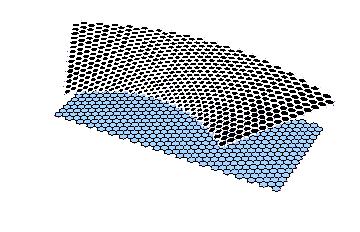
Figure 1: (Color online). Sketch of the suggested bending geometry that would generate a uniform pseudomagnetic field and open band gaps in graphene’s electronic spectrum. The graphene rectangle (lower image) is bent into a circular arc (upper).

First, let us complete the analysis of Ref.Guinea et al., 2009 by classifying the strain distributions that are compatible with equilibrium elasticity and lead to a uniform pseudomagnetic field.

We will use the coordinates that are fixed with respect to graphene’s honeycomb lattice in such a way that the $x$ axis corresponds to a zigzag direction. In this case, the gauge field A acting on charge carriers in graphene can be written asSuzuura and Ando (2002); Mañes (2007)

$$A_{x} =\pm c\frac{\beta}{a}\left(u_{xx}-u_{yy}\right)$$

$$A_{y} =\mp 2c\frac{\beta}{a}u_{xy}$$ (1)

where $\beta=-\partial\log(t)/\partial\log(a)$, where $t\approx 3$eV is the electron hopping between $p_{z}$ orbitals located at nearest neighbor atoms, $a\approx 1.4$Å  is the distance between them, $c$ is a numerical constant that depends on the details of atomic displacements within the lattice unit cell, and $u_{ij}$ is the strain tensor. The two signs correspond to the two valleys, $K$ and $K^{\prime}$ in the Brillouin zone of graphene.

In two dimensional elasticity problems, it is convenient to study the stress tensor, $\sigma_{ij}=\partial{\cal F}/\partial u_{ij}$, where ${\cal F}$ is the elastic energyLandau and Lifschitz (1959). The gauge field can be written in terms of the stress tensor as

$$A_{x} =\pm c\frac{\beta}{2a\mu}\left(\sigma_{xx}-\sigma_{yy}\right)$$

$$A_{y} =\mp c\frac{\beta}{\mu a}\sigma_{xy}$$ (2)

where $\mu$ is a Lamé coefficient. Furthermore, possible stress distributions that describe two dimensional elastic systems in equilibrium can be written in terms of complex variables $z=x+iy$ and $\bar{z}=x-iy$ asLandau and Lifschitz (1959)

$$\sigma_{xx} =\frac{\partial^{2}f(z,\bar{z})}{\partial y^{2}}$$

$$\sigma_{yy} =\frac{\partial^{2}f(z,\bar{z})}{\partial x^{2}}$$

$$\sigma_{xy} =-\frac{\partial^{2}f(z,\bar{z})}{\partial x\partial y}$$ (3)

Here $f(z,\bar{z})$ is either the real or the imaginary part of a function

$${\cal F}(z,\bar{z})={\cal F}_{1}(z)+\bar{z}{\cal F}_{2}(z)$$ (4)

where ${\cal F}_{1}(z)$ and ${\cal F}_{2}(z)$ are analytic functions. For the case of pure shear deformations considered in Ref.Guinea et al., 2009 ${\cal F}_{2}=0$ but here we will not restrict ourselves by this limitation. Since both stress and A are given by the second derivatives of ${\cal F}$, whereas $B_{S}$ is given by the first derivatives of A, a uniform $B_{S}$ necessitates ${\cal F}$ to have a cubic dependence on the coordinates. Such a function must have the following structure:

$${\cal F}(x,y)=c_{1}(x+iy)^{3}+c_{2}(x-iy)(x+iy)^{2}$$ (5)

where $c_{1}$ and $c_{2}$ are arbitrary constants. Separating the real and imaginary part of equation (6), we find four possible functions that result in uniform $B_{S}$

$$f(x,y)\propto\left\{\begin{array}[]{c}x^{3}-3xy^{2}\\ x^{3}+xy^{2}\\ 3x^{2}y-y^{3}\\ x^{2}y+y^{3}\end{array}\right.$$ (6)

The second pair of the solutions is equivalent to the first one by swapping the axes. For the lattice orientation used in Eq. (1), the first pair leads to a gauge field such that $A_{x}\propto x$ and $A_{y}\propto y$ and, accordingly, $B_{S}$ is zero. Hence, the stress distributions that give rise to a uniform pseudomagnetic field can be expressed in terms of a superposition of the functions in lines 3 and 4. The strain configuration found in ref.Guinea et al., 2009 involves only the 3rd function $f(x,y)\propto 3x^{2}y-y^{3}$, which leads to a unique solution for the shape of graphene flake where such distribution of stresses can be created by normal forces only. Unfortunately, this solution is not easy to realize experimentally. The use of both 3rd and 4th functions offers further possibilities.

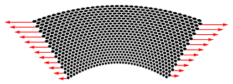
Figure 2: (Color online). Stretching geometry leading to a uniform pseudomagnetic field inside a rectangular graphene sample. Normal forces are applied at two opposite boundaries and their magnitude is indicated by the length of the plotted arrows.

In the following, we consider the deformations required to create a uniform $B_{S}$ inside a rectangular graphene crystal, of width $W$ and length $L$, with normal forces applied at the left and right boundaries as sketched in Figure 2. The non-deformed crystal fills the region $-L/2\leq x\leq L/2,-W/2\leq y\leq W/2$. Let us write the forces at the right and left boundaries $x=\pm L/2$ as

$$F_{x}^{R,L} =f_{0}^{R,L}+f_{1}^{R,L}y$$

$$F_{y}^{R,D} =0$$ (7)

The condition of zero total force and zero total torque requires $f_{0}^{R}=-f_{0}^{L}=f_{0}$ and $f_{1}^{R}=-f_{1}^{L}=f_{1}$ where $f_{0}$ and $f_{1}$ are constants. The absence of forces at the upper and lower edges implies that $\sigma_{yy}=\sigma_{xy}=0$ there. At the right and left edges, we have

$$\sigma_{xx} =\sigma_{0}\left(y+\frac{f_{0}}{f_{1}}\right)$$

$$\sigma_{xy} =0$$ (8)

where $\sigma_{0}$ is a constant that depends on applied forces. A stress distribution within the crystal, which is compatible with these boundary conditions, is generated by a function $f(y)=C[y^{3}/3+(f_{0}/f_{1})(y^{2}/2)]$. This function can be considered as a superposition of solutions 3 and 4 of Eq. (6), which leads to a uniform $B_{S}$, and a constant term that describes a uniaxial strain and does not give rise to an additional pseudomagnetic field. The latter term ensures that the lattice is stretched everywhere, there is no possibility for out of plane deformations. Inside the rectangular crystal, $\sigma_{xx}$ depends only on $y$ in the manner described by eq. (8), and $\sigma_{yy}=\sigma_{xy}=0$. From this stress distribution, we find the lattice distortions

$$u_{x} =u_{0}\left(2xy+\frac{f_{0}}{f_{1}}x\right)$$

$$u_{y} =u_{0}\left[-x^{2}-\frac{\lambda}{\lambda+4\mu}\left(y^{2}+\frac{f_{0}}{f_{1}}y\right)\right]$$ (9)

where $u_{0}$ is a constant that defines the maximum stress. These displacements lead to the curved shape shown in Fig. 2, which was drawn using the reportedZakharchenko et al. (2009) Lamé coefficients of graphene, $\lambda\approx 3.3$eV Å^-2 and $\mu\approx 9.4$eV Å^-2. The maximum strain occurs at the top and bottom boundaries and can be estimated as $\bar{u}_{max}\approx u_{0}(W+f_{0}/f_{1})$. The pseudomagnetic field inside the graphene crystal is given by

$$B_{S} =c\beta\frac{2\Phi_{0}u_{0}}{a}=c\beta\frac{\Phi_{0}\bar{u}}{aW}$$ (10)

where $\Phi_{0}$ is the flux quantum. The effective magnetic length is $\ell_{B}=\sqrt{(aW)/(\beta\bar{u})}$. This field has the same dependence on the crystal dimensions and the maximum strain as in the examples discussed in Ref.Guinea et al., 2009. For $W\approx 0.1$ micron and $\bar{u}\approx 10\%$ the generated effective field is of the order of 20T.

Experimentally, it may be difficult to create the precise stress distribution prescribed by Eq. (8). However, one can see that the required shape of the strained graphene crystal in Fig. 2 resembles an arc of a circle. To this end, we consider next the geometry in which a rectangular graphene crystal is bent into a circular arc, as sketched in Fig. 1 and shown in more detail in Fig. 3a. Note that this geometry is in fact standard for experimental studies of strain (see, e.g., Ref.Mohiuddin et al., 2009; Huang et al., 2009; Tsoukleri et al., 2009) with the only difference that the bending should be applied in plane rather than out of plane of a graphene sheet.

If the radius of the inner circle defining the lower edge in Fig. 3a is $R$, the shape of the deformed rectangle is given by

$$u_{x}(x,y) =(R+y)\sin\left[\frac{2x}{L}\arcsin\left(\frac{L}{2R}\right)\right]-x$$

$$u_{y}(x,y) =(R+y)\cos\left[\frac{2x}{L}\arcsin\left(\frac{L}{2R}\right)\right]-R-y$$ (11)

The undistorted rectangular shape is recovered for $L/R\rightarrow 0$. The displacements in Eq. (11) can be expanded in powers of $R^{-1}$, and the leading terms are

$$u_{x}(x,y) =\frac{xy}{R}$$

$$u_{y}(x,y) =-\frac{x^{2}}{2R}$$ (12)

These displacements do not exceed ${\rm max}(L,W)^{2}/R$. The next terms lead to corrections bound by ${\rm max}(L,W)^{3}/R^{2}$. The distortions in Eq. (12) coincide with those in eq. (9) in the limit of vanishing Poisson ratio $\lambda/(\lambda+2\mu)\rightarrow 0$ and lead to a uniform $B_{S}$ inside the sample. The maximum strain is $L/2R$. For an arbitrary value of $L/R$, the pseudomagnetic field is given by

$$B_{S}(x,y) =-4c\frac{\beta\Phi_{0}}{aL}\arcsin\left(\frac{L}{2R}\right)\cos\left[\frac{2x}{L}\arcsin\left(\frac{L}{2R}\right)\right]\times$$

$$\times\left[1-\frac{R+y}{L}\arcsin\left(\frac{L}{2R}\right)\right]$$ (13)

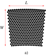
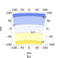
Figure 3: (Color online). (a) - Rectangular graphene sample deformed into an arc. The radii of the lower and upper edges are $R$ and $R+W$, respectively. The plot is for $R=5\times L$. (b) - Effective magnetic field, in Teslas, for the same deformed ribbon. Dimensions are $W=200$nm, $L=192$nm, $R=5\times L=960$ nm. The maximum strain is 10$\%$.

For $L/R\rightarrow 0$, the field reduces to $B_{S}\approx-c(\beta\Phi_{0})/(aR)$, in agreement with Eq. (10) and the estimates given in Ref.Guinea et al., 2009. The relative corrections to the constant value of $B_{S}$ are of the order $L/2R$, that is, the maximum strain. An example of the field distribution described by Eq. (13) is plotted in Fig. 3b.

The found strain is not purely shear but it also contains a dilatation. The latter gives rise to an effective scalar potentialSuzuura and Ando (2002), in addition to the discussed pseudomagnetic field. Below, we show that due to screening, the extra potential does not radically affect Landau quantization.

Following Ref.Suzuura and Ando, 2002, and using eqs. 9, this potential is:

$$V(x,y)=V_{0}\left(\partial_{x}u_{x}+\partial_{y}u_{y}\right)=V_{0}\left[2u_{0}y+\frac{4\mu f_{0}}{f_{1}(\lambda+4\mu)}\right]$$ (14)

where $V_{0}\approx 3$eV, estimated from the linear rise in the work function of graphene under compression between 0 and 10% strainChoi et al. (2009) (note that in Ref.Suzuura and Ando, 2002 a much larger value of 16 eV is quoted, from old experimental data on transport properties of graphite). The constant contribution gives a rigid shift to all the levels while the non uniform term is equivalent to an effective electric field along the $y$ direction. Unlike the strain induced gauge field, this potential will induce a charge redistribution and will be screened by the carriers in graphene.

We consider first the screening expected if we assume that the flake is a perfect metal, neglecting corrections due to quantum properties of the electron gas. The induced charge density, $\delta\rho(\vec{r})$ can be thus obtained from the condition

$$e^{2}\int d^{2}\vec{r}^{\prime}\frac{\delta\rho(\vec{r}^{\prime})}{|\vec{r}-\vec{r}^{\prime}|}=\frac{2V_{0}\bar{u}}{W}\delta\rho(\vec{r})y$$ (15)

This equation can be rescaled by the substitution $\delta\bar{\rho}(x/L,y/W)=(W+L)/(2L)\times(2V_{0}\bar{u})/(e^{2}W)\times\delta\rho(x,y)$. where the function $\delta\bar{\rho}(\bar{x},\bar{y})$ depends only on the aspect ratio, $W/L$.

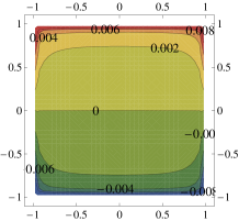
Figure 4: (Color online). Variation in density, $\delta\bar{\rho}(\bar{x},\bar{y})$, in dimensionless units (see text) due to the screened scalar potential induced by strains. The aspect ratio is $L/W=1$.

The density of carriers in a given Landau level due to the effective field given in Eq. 10, setting $c=1$, is $\rho_{LL}=2(aW)/(\beta\bar{u})$ so that $\delta\rho/\rho_{LL}=(W+L)/(2L)\times(4V_{0}a)/(\beta e^{2})\times\delta\bar{\rho}(x/L,y/W)$. Hence, the non uniform density induced by the effective field, in units of the difference in densities between different quantum Hall plateaus, is approximately given by $\delta\bar{\rho}$ shown in Fig. 4.

To provide an ideal metallic screening, the chemical potential should coincide at each point with the positions of one of the Landau levels. Hence, the quantum energy of the carriers is larger than in a uniform electron distribution, when the Fermi energy lies in a pseudogap between the Landau levels. Thus, in addition to the classical screening energy, discussed above, we also must add the change in energy due to the changes in occupancies of the electron levels in the presence of the scalar potential. We first assume that the induced electronic density is given by the solution of Eq. 15, and that the electronic states are the Landau levels induced by the effective field in Eq. 10. Then, the two contributions to the energy, for $W\sim L$, are of the order:

$$E_{elec} \sim\frac{(V_{0}\bar{u})^{2}L}{e^{2}}\langle|\delta\bar{\rho}|\rangle^{2}$$

$$E_{quantum} \sim\frac{v_{F}\beta V_{0}\bar{u}^{2}}{e^{2}}\langle|\delta\bar{\rho}|\rangle\sqrt{\frac{L}{a}}$$ (16)

The calculations shown in Fig. 4 suggest that $\langle|\delta\bar{\rho}|\rangle=f\approx 10^{-2}-10^{-1}$, and $v_{F}\sim e^{2}\sim V_{0}a$. Then, the scalar potential is screened, and the process can be described by the classical model outlined earlier, if $\sqrt{L/a}\gtrsim f^{-1}$, that is, $L\gtrsim 10^{2}-10^{3}$nm. For smaller sizes, the rigidity of the quantum levels induced by the gauge potential prevents any rearrangement of the charge inside the flake. A detailed theory of screening in this situation will be presented elsewhere. In either case, the electronic states are well described by the effective Landau levels induced by the field in Eq. 10.

To create the required strain experimentally, one can think of depositing graphene ribbons onto a rectangular elastic substrate and deform it in the manner prescribed by eq. (9) or by bending it into a circular arc (Fig. 1). Crystals rigidly attached to the substrate can then be of arbitrary shape, as the strain distribution in the substrate would project onto graphene and give rise to a (nearly) uniform $B_{S}$. Note that macroscopic substrates would require the use of rubber-like materials capable of withstanding very large strains, such that local deformations projected on a submicron graphene crystals could still reach  $\approx 10\%$.

$Acknowledgements$ - FG acknowledges support from MICINN (Spain) through grants FIS2008-00124 and CONSOLIDER CSD2007-00010, and by the Comunidad de Madrid, through CITECNOMIK. MIK acknowledges support from FOM (the Netherlands). This work was also supported by EPSRC (UK), ONR, AFOSR, and the Royal Society. We are thankful to Y.-W. Son for useful insights concerning Choi et al. (2009) and related work.

References

- Castro Neto et al. (2009) A. H. Castro Neto, F. Guinea, N. M. R. Peres, K. S. Novoselov, and A. K. Geim, Rev. Mod. Phys. 81, 109 (2009).
- Geim (2009) A. K. Geim, Science 324, 1530 (2009).
- Lee et al. (2008) C. Lee, X. Wei, J. W. Kysar, and J. Hone, Science 321, 385 (2008).
- Booth et al. (2008) T. J. Booth, P. Blake, R. R. Nair, D. Jiang, E. W. Hill, U. Bangert, A. Bleloch, M. Gass, K. S. Novoselov, M. I. Katsnelson, and A. K. Geim, Nano Lett. 8, 2442 (2008).
- Bunch et al. (2008) J. S. Bunch, S. S. Verbridge, J. S. Alden, A. M. van der Zande, J. M. Parpia, H. G. Craighead, and P. L. McEuen, Nano Lett. 8, 2458 (2008).
- Kim et al. (2009) K. S. Kim, Y. Zhao, H. Jang, S. Y. Lee, J. M. Kim, K. S. Kim, J. H. Ahn, P. Kim, J.-Y. Choi, and B. H. Hong, Nature 457, 706 (2009).
- Teague et al. (2009) M. L. Teague, A. P. Lai, J. Velasco, C. R. Hughes, A. D. Beyer, M. W. Bockrath, C. N. Lau, and N.-C. Yeh, Nano Lett. 9, 2542 (2009).
- Mohiuddin et al. (2009) T. M. Mohiuddin, A. Lombardo, R. R. Nair, A. Bonetti, G. Savini, R. Jalil, N. Bonini, D. M. Basko, C. Galiotis, N. Marzari, K. S. Novoselov, A. K. Geim, and A. C. Ferrari, Phys. Rev. B 79, 205433 (2009).
- Bao et al. (2009) W. Bao, F. Miao, Z. Chen, H. Zhang, W. Jang, C. Dames, and C. N. Lau, Nature Nanotechnology 4, 562 (2009).
- Huang et al. (2009) M. Huang, H. Yan, C. Chen, D. Song, T. F. Heinz, and J. Hone, Proc. Nat. Ac. Sci. (USA) 106, 7304 (2009).
- Tsoukleri et al. (2009) G. Tsoukleri, J. Parthenios, K. Papagelis, R. Jalil, A. C. Ferrari, A. K. Geim, K. S. Novoselov, and C. Galiotis, Small (2009), DOI: 10.1002/smll.200900802.
- Pereira et al. (2009) V. M. Pereira, A. H. C. Neto, and N. M. Peres, Phys. Rev. B 80, 045401 (2009).
- de Andrés and Vergés (2008) P. L. de Andrés and J. A. Vergés, Appl. Phys. Lett. 93, 171915 (2008).
- Fogler et al. (2008) M. M. Fogler, F. Guinea, and M. I. Katsnelson, Phys. Rev. Lett. 101, 226804 (2008).
- Pereira and Castro Neto (2009) V. M. Pereira and A. H. Castro Neto, Phys. Rev. Lett. 103, 046801 (2009).
- Boukhvalov and Katsnelson (2009) D. W. Boukhvalov and M. I. Katsnelson, J. Phys. Chem. C 113, 14176 (2009).
- Choi et al. (2009) S.-M. Choi, S.-H. Jhi, and Y.-W. Son (2009), eprint arXiv:0908.0977.
- Viana-Gomes et al. (2009) J. Viana-Gomes, V. M. Pereira, and N. M. Peres (2009), eprint arXiv:0909.4799.
- Mohr et al. (2009) M. Mohr, K. Papagelis, J. Maultzsch, and C. Thomsen (2009), eprint arXiv:0908.0895.
- Ribeiro et al. (2009) R. M. Ribeiro, V. M. Pereira, N. M. Peres, P. R. Briddon, and A. H. Castro Neto (2009), eprint arXiv:0905.1573.
- Farjam and Rafii-Tabar (2009) M. Farjam and H. Rafii-Tabar (2009), eprint arXiv:0909.5052.
- Suzuura and Ando (2002) H. Suzuura and T. Ando, Phys. Rev. B 65, 235412 (2002).
- Mañes (2007) J. L. Mañes, Phys. Rev. B 76, 045430 (2007).
- Guinea et al. (2009) F. Guinea, M. I. Katsnelson, and A. K. Geim (2009), Nature Physics, DOI:10.1038/NPHYS1420.
- Landau and Lifschitz (1959) L. D. Landau and E. M. Lifschitz, Theory of Elasticity (Pergamon Press, Oxford, 1959).
- Zakharchenko et al. (2009) K. V. Zakharchenko, M. I. Katsnelson, and A. Fasolino, Phys. Rev. Lett. 102, 046808 (2009).