Advectional enhancement of eddy diffusivity under parametric disorder

Abstract

Frozen parametric disorder can lead to appearance of sets of localized convective currents in an otherwise stable (quiescent) fluid layer heated from below. These currents significantly influence the transport of an admixture (or any other passive scalar) along the layer. When the molecular diffusivity of the admixture is small in comparison to the thermal one, which is quite typical in nature, disorder can enhance the effective (eddy) diffusivity by several orders of magnitude in comparison to the molecular diffusivity. In this paper we study the effect of an imposed longitudinal advection on delocalization of convective currents, both numerically and analytically; and report subsequent drastic boost of the effective diffusivity for weak advection.

Special Issue: Article preparation, IOP journals

Disorder in operation conditions of a dynamic system is known to be able to play not only trivial destructive role, distorting the system behavior, but also constructive one, inducing certain degree of order and leading to various non-trivial effects: Anderson localization [1, 2, 3, 4], stochastic [5] and coherence resonances [6], noise-induced synchronization [7], etc. One of the most distinguished and fair effects is the Anderson localization (AL), which is the localization of states in spatially extended linear systems subject to a frozen parametric disorder (random spacial inhomogeneity of parameters). AL was first discovered and discussed for quantum systems [1]. Later on, investigations were extended to diverse branches of semiclassical and classical physics: wave optics [3], acoustics [4], etc. The phenomenon was comprehensively studied and well understood mathematically for the Schrödinger equation and related mathematical models [2, 8, 9]. The role of nonlinearity in these models was addressed in literature as well (e.g., [9, 10]).

While extensively studied for conservative media, the localization phenomenon did not receive comparable attention for active/dissipative ones, like in problems of thermal convection or reaction-diffusion. The main reason is that the physical interpretation of formal solutions to the Schrödinger equation is essentially different from that of governing equations for active/dissipative media; therefore, the theory of AL may be extended to the latter only under certain strong restrictions (see [11, 12] for reference). Nevertheless, effects similar to AL can be observed in fluid dynamical systems [11, 12]. In [12] we addressed the problem where localized thermoconvective currents excited in a horizontal porous layer under frozen parametric disorder (spacial inhomogeneity of the macroscopic permeability, the heat diffusivity, etc.) drastically influence the process of transport of a passive scalar (e.g., a pollutant) along the layer. Below the threshold of instability of the disorder-free system, the effective diffusivity quantifying this transport has been found to be faithfully determined by localization properties of patterns. Meanwhile, in [11] these properties have been revealed to be greatly affected by a weak imposed longitudinal advection. Hence, one can expect a weak advection to lead to a significant enhancement of the effective diffusivity of a nearly indiffusive pollutant. Treatment of this effect is the subject of the present paper.

The paper is organized as follows. In section 1 we formulate the specific physical problem that we deal with and introduce the relevant mathematical model; in particular, we discuss disorder-induced excitation of localized currents below the instability threshold of the disorder-free system and advectional delocalization of these patterns. Section 2 presents the results of a numerical simulation and calculation of the effective diffusivity. In section 3 we develop an analytical theory for the effective diffusivity in the presence of an imposed advection. Section 4 ends the paper with conclusions.

1 Problem formulation and current state of research

In nature and technology, a broad variety of active media where pattern selection occurs is governed by Kuramoto–Sivashinsky type equations. In the presence of an imposed advectional transport $u$ in the $x$-direction the modified Kuramoto–Sivashinsky equation reads

$$\dot{\theta}(x,t)=-\left(u\,\theta(x,t)+\theta_{xxx}(x,t)+q(x)\,\theta_{x}(x,t)-(\theta_{x}(x,t))^{3}\right)_{x}.$$ (1)

This equation describes two-dimensional large-scale natural thermal convection in a horizontal fluid layer heated from below [13, 14] and is still valid for a turbulent fluid [15], a binary mixture at small Lewis number [16], a porous layer saturated with a fluid [17], etc. In these fluid dynamical systems, except for the turbulent one [15], the plates bounding the layer should be nearly thermally insulating (in comparison to the fluid) for a large-scale convection to arise. In the problems mentioned, equation (1) governs evolution of temperature perturbations $\theta$ which are nearly uniform along the vertical coordinate $z$ and determine fluid currents.

The origin of such a frequent occurrence of equation (1) is its general validity, which may be argued as follows. Basic laws in physics are conservation ones. This often results in final governing equations having the form $\partial_{t}[\mbox{quantity}]+\nabla\!\cdot\![\mbox{flux of quantity}]=0$. Such conservation laws lead to Kuramoto–Sivashinsky type equations. While the original Kuramoto–Sivashinsky equation has a quadratic nonlinear term (cf [18]), this term should be replaced by a cubic one for the systems with the sign inversion symmetry of the fields, which is widespread in nature, or for description of a spatiotemporal modulation of an oscillatory mode. Thus the governing equation takes the form (1). On these grounds, we state that equation (1) describes pattern formation in a broad variety of physical systems.

We restrict this paper to the case of convection in a porous medium [17, 12] for the sake of definiteness; nonetheless, most of our results may be extended in a straightforward manner to the other physical systems mentioned. Equation (1) is already dimensionless and below we introduce all parameters and variables in appropriate dimensionless forms.

In the large-scale (or long-wavelength) approximation, which we use, the characteristic horizontal scales are assumed to be large against the layer height $h$. In equation (1), $q(x)$ represents the local supercriticality: $(21/2)h^{2}q(x)$ is the sum of relative deviations of the heating intensity and of the macroscopic properties of the porous matrix (porosity, permeability, heat diffusivity, etc.) from the critical values for the spatially homogeneous case [17]. For positive spatially uniform $q$, convection sets up, while for negative $q$, all the temperature perturbations decay. In a porous medium [17], the macroscopic fluid velocity field is

$$\vec{v}=\frac{\partial\Psi}{\partial z}\vec{e}_{x}-\frac{\partial\Psi}{\partial x}\vec{e}_{z}\,,\qquad\Psi=\frac{3\sqrt{35}}{h^{3}}\,z(h-z)\,\theta_{x}(x,t)\equiv f(z)\,\psi(x,t)\,,$$ (2)

where $\psi(x,t)\equiv\theta_{x}(x,t)$ is the stream function amplitude, and the reference frame is such that $z=0$ and $z=h$ are the lower and upper boundaries of the layer, respectively [figure 1(b)]. Though the temperature perturbations obey equation (1) for diverse convective systems, function $f(z)$, which determines the relation between the flow pattern and the temperature perturbation, is specific to each case. Notice that $u$ is not presented in expression (2) owing to its smallness in comparison to the excited convective currents $\vec{v}$. The impact of a weak imposed advective flow on the evolution of temperature perturbations is caused by its symmetry properties: the gross advective flux through the vertical cross-section is $u$, while the convective flow $\vec{v}$ possesses zero gross flux and, therefore, yields a less effective heat transfer along the layer [17].

(a)
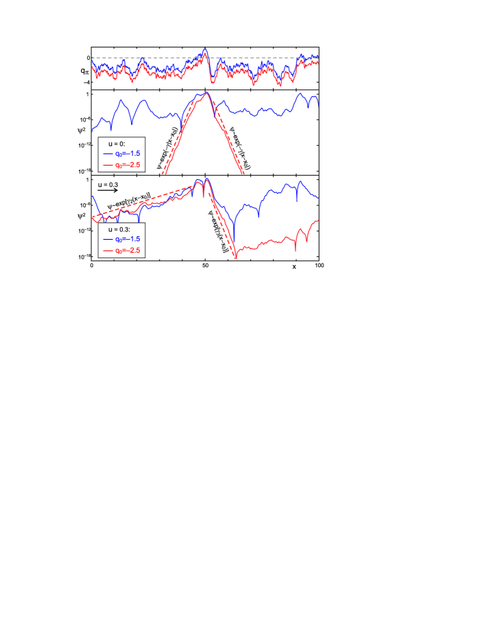
(b)

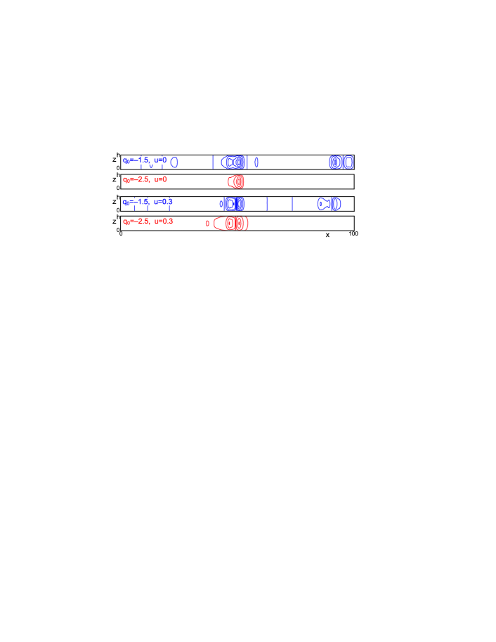
Figure 1: (a) Establishing steady solutions to equation (1) are sets of exponentially localized patterns [shown for one and the same realization of random inhomogeneity $\xi(x)$ and $\varepsilon=1$; $q(x)$ is represented by $q_{\pi}(x)=\pi^{-1}\int_{x-\pi/2}^{x+\pi/2}q(x^{\prime})\rmd x^{\prime}$].
(b) The stream lines corresponding to the solutions in graph (a) are plotted for the case of convection in a porous layer [see equation (2) for an exact relation].

Although equation (1) is valid for a large-scale inhomogeneity $q(x)$, which means $h|q_{x}|/|q|\ll 1$, one can set such a hierarchy of small parameters, namely $h\ll(h|q_{x}|/|q|)^{2}\ll 1$, that a frozen random inhomogeneity may be represented by white Gaussian noise $\xi(x)$:

$$q(x)=q_{0}+\xi(x),\quad\left\langle\xi(x)\right\rangle=0,\quad\left\langle\xi(x)\xi(x^{\prime})\right\rangle=2\varepsilon^{2}\delta(x-x^{\prime}),$$

where $\varepsilon^{2}$ is the disorder intensity and $q_{0}$ is the mean supercriticality (i.e. departure from the instability threshold of the disorder-free system). Numerical simulation reveals only time-independent solutions to establish in (1) with $u=0$ and such $q(x)$ [11]; for a small non-zero $u$, stable oscillatory regimes are of low probability by continuity.

In the stationary case for $u=0$ the linearized form of equation (1), i.e.,

$$-\theta_{xxx}(x)-\xi(x)\,\theta_{x}(x)=q_{0}\,\theta_{x}(x)\,,$$ (3)

is a stationary Schrödinger equation for $\psi=\theta_{x}$ with $q_{0}$ instead of the state energy and $-\xi(x)$ instead of the potential. Therefore, similarly to the case of the Schrödinger equation (see [2, 8, 9]), all the solutions $\psi(x)$ to the stationary linearized equation (1) are spatially localized for arbitrary $q_{0}$; asymptotically,

$$\psi(x)\propto\exp(-\gamma|x|),$$

where $\gamma$ is the localization exponent. Such a localization can be readily seen for the solution to the nonlinear problem (1) in figure 1(a) for $q_{0}=-2.5$, $u=0$, which is a solitary vortex.

Figure 2: Spectrum of localization exponents of time-independent patterns for $\varepsilon=1$, $q_{0}=-1$ derived from equation (4) [11].

For $u\neq 0$ the solitary patterns are still exponentially localized [figure 1(a), $u=0.3$]. However, their localization properties change drastically because instead of the second-order linear ODE with respect to $\psi=\theta_{x}$, equation (3), one finds a third-order equation:

$$-u\theta(x)-\theta_{xxx}(x)-\xi(x)\,\theta_{x}(x)=q_{0}\,\theta_{x}(x)\,.$$ (4)

The two symmetric modes $\theta\propto\exp(\pm\gamma x)$ and trivial solution $\theta=const$ ($\psi=0$) turn into three modes $\theta\propto\exp(\gamma_{i}x)$, $\gamma_{3}<0<\gamma_{2}<\gamma_{1}$, of equation (4) with $u>0$, $q_{0}<0$ (see sample spectrum of $\gamma_{i}$ in figure 2; cf [11] for details). Specifically, $\gamma_{1}$-mode is the successor of $+\gamma$, $\gamma_{2}$-mode is the one of the trivial homogeneous mode, and $\gamma_{3}$-mode is that of $-\gamma$. Thus, the upstream flank of the localized pattern is now composed by two modes decaying in the distance from the pattern:

$$\theta(x)\approx\Theta_{1}(x)\rme^{\gamma_{1}x}+\Theta_{2}(x)\rme^{\gamma_{2}x}\quad\mbox{ or }\quad\psi(x)\approx\gamma_{1}\widetilde{\Theta}_{1}(x)\rme^{\gamma_{1}x}+\gamma_{2}\widetilde{\Theta}_{2}(x)\rme^{\gamma_{2}x},$$

where functions $\Theta_{i}(x)$ and $\widetilde{\Theta}_{i}(x)$ neither grow nor decay over large distances. The $\gamma_{1}$-mode, which disappears for $u=0$, i.e. $\gamma_{1}=0$, decays slowly for a small finite $u$, prevails over the $\gamma_{2}$-mode decaying rapidly, and, thus, determines the upstream localization properties of the pattern. The upstream localization length $1/\gamma_{1}$ can become remarkably large leading to upstream delocalization of patterns, which can be seen in figure 1.

One should keep in mind, that consideration of solitary patterns makes sense where such patterns can be distinguished, i.e., are sparse enough in space. This is the case of negative $q_{0}\lesssim-1$. In figure 1, for a sample realization of $\xi(x)$, one can see that localized patterns can be discriminated for $\varepsilon=1$, $q_{0}=-1.5$ and the localization properties are very well pronounced for $q_{0}=-2.5$.

Here we would like to emphasize the fact of existence of convective currents below the instability threshold of the disorder-free system. These currents considerably and nontrivially affect transport of a pollutant (or other passive scalar), especially when its molecular diffusivity is small in comparison to the thermal one, which is quite typical in nature (for instance, at standard conditions the molecular diffusivity of NaCl in water is $1.1\cdot 10^{-9}m^{2}/s$ against the heat diffusivity of water which is $1.3\cdot 10^{-7}m^{2}/s$). Transport of a nearly indiffusive passive scalar, quantified by the effective (or eddy) diffusivity coefficient, is the object of our research, as a “substance” which is essentially influenced by these localized currents and, thus, provides an opportunity to observe manifestation of disorder-induced phenomena discussed in [11].

In [12] we studied the problem for the case of no advection ($u=0$) and calculated (both numerically and analytically) the enhancement of the effective diffusivity by disorder-induced currents; this enhancement is especially strong for low molecular diffusivity deep below the instability threshold of the disorder-free system (see figure 3). In this paper we address the role of an imposed advection in this problem. The interest to advection is provoked by its dramatic influence on localization properties, i.e., the upstream delocalization of convective currents that is described above. We expect this delocalization to result in a giant increase of the effective diffusivity for a nearly indiffusive pollutant and, particularly, in the lowering of the mean supercriticality ($q_{0}$) value at which the transition from sets of localized convective currents to an almost everywhere intense ‘global’ flow occurs.

2 Effective diffusivity

In this section we describe the transport of a passive pollutant by a steady convective flow (2); “passive” means that the flow is not influenced by the pollutant. The assumption of passiveness is practically relevant because (biologically/chemichally) significant concentrations of a pollutant can be very small and mechanically negligible. The flux $\vec{j}$ of the pollutant concentration $C$ is

$$\vec{j}=\vec{v}\,C-D\nabla C\,,$$ (5)

where the first term describes the convective transport, the second one represents the molecular diffusion, and $D$ is the molecular diffusivity. The establishing time-independent distributions of the pollutant obey

$$\nabla\cdot\vec{j}=0\,.$$ (6)

Equation (6) [with account for (2)] yields a distribution of $C$ which is uniform along $z$ and is determined by

$$\frac{\rmd C(x)}{\rmd x}=-\frac{J}{\displaystyle D+\frac{21\,\psi^{2}(x)}{2\,h^{2}D}}\,,$$ (7)

where $J$ is the constant pollutant flux along the layer. Detailed derivation of equation (7) for $u=0$ can be found in [12] where it was performed in the spirit of the standard multiscale method (interested readers can consult, e.g., [19, 20]). Remarkably, advection velocity $u$ is not presented in the last equation: its direct contribution to convective currents transferring the pollutant is small in comparison to the one of excited convective currents. Instead, it influences the heat transfer and, consequently, excited flows, drastically changing properties of the field $\psi(x)$. Notice that, for the other convective systems which we mentioned in section 1, the result differs only in the factor ahead of $\psi^{2}/D$.

Thus we come to introducing the effective diffusivity for the system under consideration (general ideas on the effective diffusivity in systems with irregular currents can be found, e.g., in [21, 20]). Let us consider the domain $x\in[0,L]$ with the imposed concentration difference $\delta C$ at the ends. Then the establishing pollutant flux $J$ is defined by the integral [cf (7)]

$$\delta C=-J\int\limits_{0}^{L}\frac{\rmd x}{\displaystyle D+\frac{21\,\psi^{2}(x)}{2\,h^{2}D}}\,.$$

For a lengthy domain the specific realization of $\xi(x)$ becomes insignificant:

$$\delta C=-J\,L\left\langle\left(D+\frac{21\,\psi^{2}(x)}{2\,h^{2}D}\right)^{-1}\right\rangle\equiv-\sigma^{-1}J\,L\,,$$

Hence,

$$J=-\sigma\frac{\delta C}{L},$$

which means that $\sigma$ can be treated as an effective diffusivity.

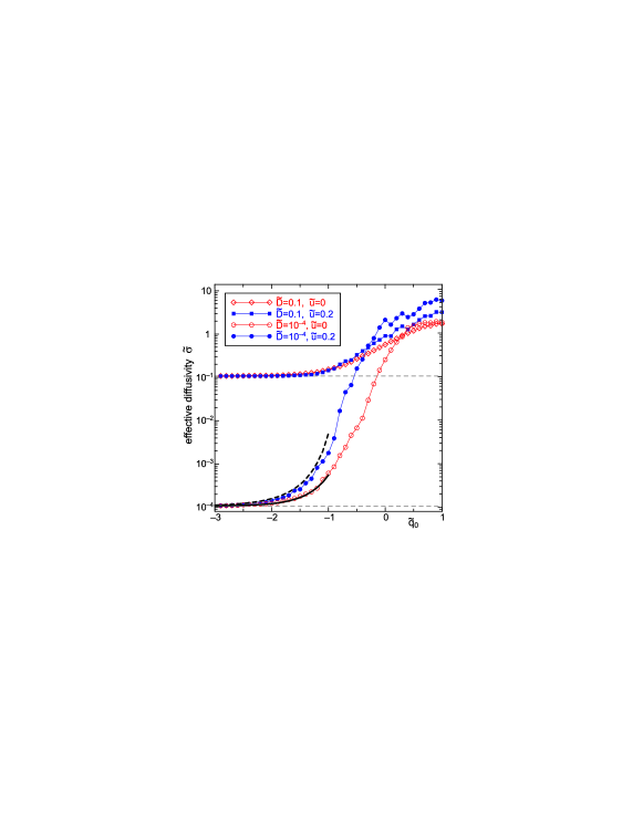
Figure 3: Dependencies of effective diffusivity $\widetilde{\sigma}$ on mean supercriticality $\widetilde{q}_{0}$ in the presence of an imposed advection ($\widetilde{u}=0.2$) and without it ($\widetilde{u}=0$). The bold black solid line represents the analytical dependence for $\widetilde{u}=0$, and the dashed line represents the one for $\widetilde{u}=0.2$ (see section 3).

The effective diffusivity

$$\sigma=\left\langle\left(D+\frac{21\,\psi^{2}(x)}{2\,h^{2}D}\right)^{-1}\right\rangle^{-1}$$ (8)

turns into $D$ for vanishing convective flow. For small $D$ the regions of the layer where the flow is damped, $\psi\ll 1$, make large contribution to the mean value appearing in (8) and diminish $\sigma$, thus, leading to the locking of the spreading of the pollutant.

The disorder strength $\varepsilon^{2}$ can be excluded from equations by the appropriate rescaling of parameters and fields. As a consequence, the results on the effective diffusivity can be comprehensively presented in terms of $\widetilde{D}$, $\widetilde{\sigma}$, $\widetilde{q}_{0}$, and $\widetilde{u}$:

$$\widetilde{D}=\sqrt{\frac{2}{21}}\,\varepsilon^{4/3}D,\qquad\widetilde{\sigma}=\sqrt{\frac{2}{21}}\,\varepsilon^{4/3}h\sigma,\qquad\widetilde{q}_{0}=\frac{q_{0}}{\varepsilon^{4/3}}\,,\qquad\widetilde{u}=\frac{u}{\varepsilon^{2}}\,.$$

Figure 3 provides calculated dependencies of effective diffusivity $\widetilde{\sigma}$ on $\widetilde{q}_{0}$ for moderate and small values of molecular diffusivity $\widetilde{D}$. Concerning these dependencies the following is worth noticing:

(a) For small $\widetilde{D}$ a quite sharp transition of effective diffusivity $\widetilde{\sigma}$ between moderate values and ones comparable with $\widetilde{D}$ occurs near $q_{0}=0$ (note logarithmic scale of the vertical axis), suggesting the transition from an almost everywhere intense ‘global’ flow to a set of localized currents to take place.

(b) In the presence of a weak imposed advection, $\widetilde{u}=0.2$, the transition to ‘global’ flow occurs at the value of $\widetilde{q}_{0}$ which is considerably lower than that without advection.

(c) Below the instability threshold of the disorder-free system, where only sparse localized currents are excited, the effective diffusion can be significantly enhanced by these currents.

(d) The disorder-induced enhancement of the effective diffusivity is especially drastic in the presence of an imposed advection; e.g., for $\widetilde{D}=10^{-4}$, $\widetilde{q}_{0}=-1$, the effective diffusivity is increased by one order of magnitude compared to the molecular diffusivity without advection ($\widetilde{u}=0$) and by two orders of magnitude for $\widetilde{u}=0.2$.

3 Analytical theory

3.1 Transport through time-independent patterns

The effective diffusivity can be analytically evaluated for a small molecular diffusivity ($\widetilde{D}\ll 1$) and sparse domains of excitation of convective currents (the spacial density of the excitation domains $\nu\ll 1$). In [12] it was evaluated for the case of no advection,

$$\widetilde{\sigma}_{\widetilde{u}=0}\approx\widetilde{D}\left(\frac{2}{\widetilde{D}}\right)^{\frac{2\nu}{\gamma}}\!\!,$$ (9)

where one can use the asymptotic expressions for the density of the excitation domains $\nu$,

$$\nu\approx\frac{1}{4\sqrt{1.95\,\pi}\,\varepsilon^{2/3}|\widetilde{q}_{0}|}\exp\left(-\frac{1.95\,\widetilde{q}_{0}^{2}}{4}\right),$$ (10)

and

$$\gamma(\widetilde{u}=0)=\varepsilon^{-\frac{2}{3}}\left(|\widetilde{q}_{0}|^{\frac{1}{2}}-\frac{1}{4}|\widetilde{q}_{0}|^{-1}-\frac{5}{32}|\widetilde{q}_{0}|^{-\frac{5}{2}}+\dots\right),$$

which are valid for $\widetilde{q}_{0}\!<\!-1$. The latter expression is known from the classical theory of AL (e.g., see [8, 9]). In the following we advance the evaluation procedure realized in [12] in order to account for the asymmetry between up- and downstream localization exponents.

Now we calculate the average

$$\frac{1}{\widetilde{\sigma}}=\left\langle\Bigg{(}\widetilde{D}+\frac{\psi^{2}(x)}{\widetilde{D}}\Bigg{)}^{-1}\right\rangle.$$

Due to ergodicity, this average over $x$ for a given realization of $\xi(x)$ coincides with the average over realizations of $\xi(x)$ at a certain point $x_{0}$. We set the origin of the $x$-axis at $x_{0}$ and find $\widetilde{\sigma}^{-1}=\langle\big{(}\widetilde{D}+\psi^{2}(0)/\widetilde{D}\big{)}^{-1}\rangle_{\xi}$.

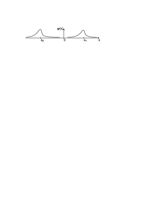
Figure 4: Sketch of two localized flow patterns being nearest to the origin.

When the two nearest to the origin excitation domains are distant and localized near $x_{1}>0$ and $x_{2}<0$ (see figure 4),

$$\psi(0)\approx\gamma_{1}\theta_{1}\rme^{-\gamma_{1}x_{1}}+\gamma_{2}\theta_{2}\rme^{-\gamma_{2}x_{1}}+\gamma_{3}\theta_{3}\rme^{-\gamma_{3}x_{2}},$$ (11)

where $\theta_{1,2}$ and $\theta_{3}$ characterize the amplitude of temperature perturbation modes excited around $x_{1}$ and $x_{2}$, respectively. For small $\widetilde{D}$ and density $\nu$, the contribution of the excitation domains to $\widetilde{\sigma}^{-1}$ is negligible against that of the extensive regions where flow is weak, but $|\psi|$ is still larger than $\widetilde{D}$. Therefore, one may be not very subtle with “cores” of excitation domains and may utilize expression (11) even for small $x_{1,2}$:

$$\frac{1}{\widetilde{\sigma}}=\left\langle\frac{1}{\widetilde{D}+\psi^{2}(0)/\widetilde{D}}\right\rangle_{\xi}$$

$$\quad=\left\langle\int\limits_{0}^{\infty}\rmd x_{1}\int\limits_{0}^{\infty}\rmd x_{2}\frac{p(x_{1})\,p(x_{2})}{\widetilde{D}+\widetilde{D}^{-1}(\gamma_{1}\theta_{1}\rme^{-\gamma_{1}x_{1}}+\gamma_{2}\theta_{2}\rme^{-\gamma_{2}x_{1}}+\gamma_{3}\theta_{3}\rme^{\gamma_{3}x_{2}})^{2}}\right\rangle_{\theta_{1},\theta_{2}}$$ (12)

where $p(x_{1})$ [ $p(x_{2})$] is the density of the probability to observe the nearest right [left] excitation domain at $+x_{1}$ [$-x_{2}$]. For probability distribution $P(x_{1}\!>\!x)$, one finds $P(x_{1}\!>\!x+\rmd x)=P(x_{1}\!>\!x)\,(1-\nu\rmd x)$, i.e., $(\rmd/\rmd x)P(x_{1}\!>\!x)=-\nu P(x_{1}\!>\!x)$. Hence, $P(x_{1}\!>\!x)=\rme^{-\nu x}$, and probability density $p(x)=|(\rmd/\rmd x)P(x_{1}\!>\!x)|=\nu\rme^{-\nu x}$. As regards averaging over $\theta_{i}$, it is important that the multiplication of $\theta_{i}$ by factor $F$ is effectively equivalent to the shift of the excitation domain by $|\gamma_{i}|^{-1}\ln{F}$, which is insignificant for $F\sim 1$ in the limit case that we consider. Hence, one can assume $\theta_{i}=\pm 1$ (the topological difference between different combinations of signs of $\theta_{i}$ is not to be neglected) and rewrite equation (12) as

$$\frac{1}{\widetilde{\sigma}}=\frac{1}{2}\int\limits_{0}^{\infty}\rmd x_{1}\int\limits_{0}^{\infty}\rmd x_{2}\,\nu^{2}\rme^{-\nu(x_{1}+x_{2})}\left[\frac{1}{\widetilde{D}+\widetilde{D}^{-1}(\gamma_{1}\rme^{-\gamma_{1}x_{1}}+\gamma_{2}\rme^{-\gamma_{2}x_{1}}+\gamma_{3}\rme^{\gamma_{3}x_{2}})^{2}}\right.$$

$$\hskip 113.81102pt\left.{}+\frac{1}{\widetilde{D}+\widetilde{D}^{-1}(\gamma_{1}\rme^{-\gamma_{1}x_{1}}+\gamma_{2}\rme^{-\gamma_{2}x_{1}}-\gamma_{3}\rme^{\gamma_{3}x_{2}})^{2}}\right].$$

For $\nu/\gamma_{i}\ll 1$ and $\gamma_{2}$-mode dominating over $\gamma_{1}$-mode (that is the case in figure 1), the last formula yields

$$\widetilde{\sigma}\approx\widetilde{D}\left(\frac{\gamma_{2}}{\widetilde{D}}\right)^{\frac{\nu}{\gamma_{2}}}\left(\frac{|\gamma_{3}|}{\widetilde{D}}\right)^{\frac{\nu}{|\gamma_{3}|}}\!\!.$$ (13)

Here we assume that advection is weak and suppresses thermal convection in a negligible fraction of the excitation centers and the asymptotic expression (10) is still valid.

Figure 5: The theoretical dependence of effective diffusivity $\widetilde{\sigma}$ on mean supercriticality $\widetilde{q}_{0}$ and molecular diffusivity $\widetilde{D}$ in the presence of an imposed advection, $\widetilde{u}=0.2$ (black “wireframe” surface), and without it, $\widetilde{u}=0$ (gray surface).

Noticeable difference between equation (13) for $\widetilde{u}=0$, i.e., $\gamma_{2}=-\gamma_{3}=\gamma$, and equation (9) is actually insignificant up to our approximations, because moderate number $\gamma/2$ risen to small power $2\nu/\gamma$, $(\gamma/2)^{2\nu/\gamma}$ which is the ratio of these equations, approximately equals 1. For instance, in figure 3, the curves given by analytic expressions (9) and (13) with $\gamma_{2}=-\gamma_{3}=\gamma$ are visually undistinguishable.

For small finite $\widetilde{u}$, smallness of $\gamma_{2}$ in equation (13) gives rise to a significant enhancement of effective diffusivity $\widetilde{\sigma}$, which is in agreement with the results of numerical simulation presented in figure 3. Figure 5 shows that for $\widetilde{u}=0.2$ the effective diffusivity in the presence of advection is always stronger than without it; the larger the difference between the effective and the molecular diffusivity the stronger advectional enhancement of the effective diffusivity is. For instance, for $\widetilde{D}\approx 10^{-4}$, $\widetilde{q}_{0}=-1$ the effective diffusivity in the presence of advection $\widetilde{u}=0.2$ is by factor 10 larger than without advection, and this factor grows as $\widetilde{D}$ decreases.

Noteworthy, for $\widetilde{u}=0.2$ expression (13) provides slightly overestimated value of the effective diffusivity while for $\widetilde{u}=0$ the analytical estimation is accurate. The inaccuracy appears because in our analytical theory we ignore three factors: (a) decrease of the spatial density of the excitation centers owing to advectional suppression (washing-out) of weak excitation centers; (b) for small $\widetilde{u}$ the rapidly decaying upstream $\gamma_{1}$-mode is significant because of the smallness of the slowly decaying $\gamma_{2}$-mode; and (c) as the advection strengthens, currents in some excitation domains disappear via a Hopf bifurcation [11] and thus there is non-zero probability to observe oscillatory flows for small $\widetilde{u}$ even though there is no stable time-dependent solutions for $\widetilde{u}=0$. Unfortunately, inaccuracies caused by these three assumptions can not be minimized simultaneously: the first and third assumptions require $\widetilde{u}\to 0$, while the second one needs $\widetilde{u}$ to be small but finite.

(a)  (b)

Figure 6: (a) Sample of an oscillatory flow appearing for $u=0.2$, $\varepsilon=1$: at $\widetilde{q}_{0}=-1.5$ the pattern is time-independent, further, as $\widetilde{q}_{0}$ decreases, it turns oscillatory ($\widetilde{q}_{0}=-1.6$, shown at a certain moment of time) and then decays for $\widetilde{q}_{0}\lesssim-1.7$.
(b) The effective diffusivity coefficients calculated over a short domain (length $L=100$), with sample $\xi(x)$ and the patterns plotted in graph (a), are compared with the one in the limit of an infinite domain ($L=10^{5}$).

3.2 Discussion of transport through oscillatory patterns

Oscillatory localized patterns discovered in the dynamic system (1) for non-zero $\widetilde{u}$ (figure 6(a); see [11] for details) are statistically improbable and rare when $\widetilde{u}$ is small. Notably, their relative contribution to the effective diffusivity is much larger than their fraction among the excited localized patterns. In figure 6(b) one can see the soaring of the effective diffusivity along a finite region as a localized pattern turns oscillatory ($\widetilde{q}_{0}=-1.6$) before disappearing ($\widetilde{q}_{0}\lesssim-1.7$). Figure 6(a) reveals the origin of this soaring: the oscillatory pattern is not so well localized as the time-independent one. Indeed, the localization properties of the oscillatory pattern of frequency $\omega$ are determined by the following linearization of equation (1):

$$i\omega\theta=-(u\theta+\theta_{xxx}+(q_{0}+\xi(x))\theta_{x})_{x}\,.$$ (14)

In contrast to (4), this is already a 4th-order differential equation, which yields four localization exponents. The newly appeared 4th mode possesses $\gamma\propto\omega\propto u$, i.e., decays slowly, and contributes to the downstream flank of localized patterns (evidence of these facts is beyond the scope of this paper and will be presented elsewhere). As well as the $\gamma_{2}$-mode results in upstream delocalization of time-independent patterns, the new mode leads to downstream delocalization of oscillatory patterns, which appear to be weakly localized both up- and downstream, as one sees this in figure 6(a).

Nevertheless, owing to the smallness of the fraction of the oscillatory patterns among all the localized patterns at small $\widetilde{u}$, their contribution to the effective diffusivity over large domains is still negligible. This is additionally confirmed by the accuracy of our analytical theory disregarding oscillatory currents [equation (13)]. Meanwhile, the analytical theory accounting for the oscillatory patterns should involve the distribution of frequencies of excited patterns, which are to be determined only from the nonlinear problem (1): this is not an analytically solvable problem.

4 Conclusion

We have studied the transport of a pollutant in a horizontal fluid layer by spatially localized two-dimensional thermoconvective currents appearing under frozen parametric disorder in the presence of an imposed longitudinal advection. Though we have considered the specific physical system, a horizontal porous layer saturated with a fluid and confined between two nearly thermally insulating plates, our results can be in a straightforward manner extended to a broad variety of fluid dynamical systems (like ones studied in [13, 14, 15, 16]). We have calculated numerically the dependence of the effective diffusivity on the molecular one and the mean supercriticality for a non-zero advection strength (see figure 3). The results reveal that advectional delocalization of convective currents greatly assists transfer of a nearly indiffusive pollutant ($D\ll 1$) below the instability threshold of the disorder-free system: the effective diffusivity can become by several orders of magnitude larger in comparison to that without advection.

The analytical theory focusing on advectional delocalization of localized current patterns yields results which are in a fair agreement with the results of numerical simulation. This correspondence confirms our treatment of importance of disorder-induced patterns and their localization properties in active/dissipavite media, which provoked works [11, 12].

References

References

- [1] Anderson P W 1958 Phys. Rev.109 1492–505
- [2] Fröhlich J and Spencer T 1984 Phys. Rep. 103 9–25
- [3] van Rossum M C W and Nieuwenhuizen Th M 1999 Rev. Mod. Phys.71 313–71
- [4] Maynard J D 2001 Rev. Mod. Phys.73 401–17
- [5] McNamara B and Wiesenfeld K 1989 Phys. Rev.A 39 4854–69 Gammaitoni L, Hanggi P, Jung P and Marchesoni F 1998 Rev. Mod. Phys.70 223–87
- [6] Pikovsky A S and Kurths J 1997 Phys. Rev. Lett.78 775–8
- [7] Teramae J N and Tanaka D 2004 Phys. Rev. Lett.93 204103 Goldobin D S and Pikovsky A S 2005 Physica A 351 126–32 Goldobin D S and Pikovsky A 2005 Phys. Rev.E 71 045201(R)
- [8] Lifshitz I M, Gredeskul S A and Pastur L A 1988 Introduction to the Theory of Disordered Systems (New York: Wiley).
- [9] Gredeskul S A and Kivshar Yu S 1992 Phys. Rep. 216 1–61
- [10] Pikovsky A S and Shepelyansky D L 2008 Phys. Rev. Lett.100 094101
- [11] Goldobin D S and Shklyaeva E V, Localization and advectional spreading of convective flows under parametric disorder, Phys. Rev.E submitted [arXiv:0804.3741]
- [12] Goldobin D S and Shklyaeva E V 2009 J. Stat. Mech.: Theory Exp. P01024
- [13] Knobloch E 1990 Physica D 41 450–79
- [14] Shtilman L and Sivashinsky G 1991 Physica D 52 477–88
- [15] Aristov S N and Frik P G 1989 Fluid Dynamics 24(5) 690–5
- [16] Schöpf W and Zimmermann W 1989 Europhys. Lett. 8 41–6 Schöpf W and Zimmermann W 1993 Phys. Rev.E 47 1739–64
- [17] Goldobin D S and Shklyaeva E V 2008 Phys. Rev.E 78 027301
- [18] Michelson D 1986 Physica D 19 89–111
- [19] Bensoussan A, Lions J L and Papanicolaou G 1978 Asymptotic Analysis for Periodic Structures (Amsterdam: North-Holland)
- [20] Majda A J and Kramer P R 1999 Phys. Rep. 314 238–574
- [21] Frisch U 1995 Turbulence: The Legacy of A. N. Kolmogorov (Cambridge: Cambridge University Press) p 226