TU-854

Octorber, 2009

Measurement of the Superparticle Mass Spectrum
in the Long-Lived Stau Scenario at the LHC

Takumi Ito, Ryuichiro Kitano and Takeo Moroi

Department of Physics, Tohoku University, Sendai 980-8578, Japan

1 Introduction

Signatures of supersymmetry (SUSY) at the LHC experiments crucially depend on what the lightest supersymmetric particle (LSP) is. Many of studies have assumed a neutralino as the LSP motivated by a possible explanation of dark matter of the universe. In this case, final states of SUSY events will be accompanied by missing momentum carried away by two neutralinos. The mass determinations of SUSY particles in such cases are not a straightforward task. One needs to combine various measurements to extract the masses out of observables.

Situation drastically changes when we assume that the scalar tau lepton (stau) is lighter than the lightest neutralino and thus long-lived. First, one can discover the stau by looking for anomalous tracks at the inner tracker and the muon detector [1, 2, 3]. Their momenta and velocities can be measured by analyzing the tracks, with which one can measure the stau mass with a good accuracy [4, 5, 6, 7]. The momentum information enables us to perform precise determination of the properties of SUSY particles such as masses of other superparticles [8, 9, 10, 11], the spin of the stau [12], the lifetime of the stau [13, 14, 15, 16] and P/CP/T violations in the SUSY interactions [17].

The long-lived stau is not just motivated as a golden scenario for collider experiments. There are many underlying models and parameter spaces in them to realize the scenario. Examples include the familiar ones such as supergravity and gauge mediation models. The lifetime of stau depends on details of the microscopic models; the stau can decay into a gravitino and a tau lepton if kinematically allowed or into standard model particles if $R$-parity is violated. There is a cosmological constraint on the stau lifetime from Big-Bang nucleosynthesis, but it can easily be evaded unless the lifetime is extremely long such as greater than $O(1000\ {\rm sec})$ [18].

Once the stau tracks are discovered and the measurement of the stau mass is done at the LHC, the next important quantities to measure will be other superparticle masses. In particular, measurements of selectron and smuon masses tell us about how special the third generation is in the microscopic interactions between the SUSY breaking and the standard model sectors. Even if the strength of the Yukawa interaction is the only difference between the stau and the first two generations, the mass splitting contains the information on the size of the Yukawa interaction (i.e., $\tan\beta$) and also the size of the quantum corrections to the masses (i.e., the messenger scale). An even more interesting quantity will be the mass splitting between the selectron and the smuon. Since the Yukawa coupling constants are small, a large splitting of more than $O(100\ {\rm MeV})$ level requires an explanation from a microscopic theory.

The mass measurements of superparticles in the long-lived stau scenario was first studied in [8]. They used a parameter point in the gauge-mediation model where the selectron, the smuon, and the stau are all long-lived due to a small mass splittings among three sleptons ($m_{\tilde{e}}\sim m_{\tilde{\mu}}\sim m_{\tilde{\tau}}$). Recently, the case with a long-lived selectron with a nearly degenerate smuon ($m_{\tilde{e}}\sim m_{\tilde{\mu}}<m_{\tilde{\tau}}$) was studied in [11], there it was proposed to measure the mass splitting between the smuon and the selectron by looking at the peak locations of the $e\tilde{e}$ and $\mu\tilde{e}$ invariant masses.

In this paper, we propose a method to measure the masses of superparticles in the case where $m_{\tilde{\tau}}<m_{\tilde{e}}\sim m_{\tilde{\mu}}<m_{\chi^{0}}$ in the long-lived stau scenario at the LHC. When the mass differences between the stau and other sleptons are larger than $\sim 10\ {\rm GeV}$, the decay products are hard enough to be detected, contrasted to the previous studies. This level of mass splitting is a natural expectation in many models especially for large values of the $\tan\beta$ parameter (which is somewhat motivated by the Higgs boson mass bound).

At the LHC, staus are mainly produced at the last step of the cascade-decay chains such as the neutralino decay $\chi^{0}\to\tau\tilde{\tau}$ and the chargino decay $\chi^{\pm}\to\tilde{\tau}\nu$. It has been demonstrated in various models that the neutralino mass(es) can be measured by looking for an endpoint of the $j_{\tau}$-$\tilde{\tau}$ invariant mass distribution [8, 9, 10] (where $j_{\tau}$ is $\tau$-tagged jet). We first follow this analysis and point out usefulness of the charge information of the $\tau$-jets in this study. We next show that the measured neutralino mass in turn can be used to determine the smuon and selectron masses by reconstructing the decay chains: $\chi^{0}\to\mu\tilde{\mu}\to\mu(\tilde{\tau}\tau\mu)$ and $\chi^{0}\to e\tilde{e}\to e(\tilde{\tau}\tau e)$ followed by a $\tau$ decay. We use the hadronic $\tau$ decay for the analysis. Although there are invisible neutrinos from $\tau$ decays, four-momentum of $\tau$ can be reconstructed in the event-by-event basis by using the knowledge of the neutralino mass under an assumption that the neutrino is emitted along the direction of the $\tau$-jet (which is valid when $\tau$ is highly boosted). The smuon and selectron masses can then be measured in each event up to a combinatorics. Therefore, we can see sharp peaks at the smuon and selectron masses in the distributions of the $\tilde{\tau}\tau\mu$ and $\tilde{\tau}\tau e$ invariant masses, respectively. We demonstrate that the masses and the mass difference can be measured with accuracies of $O(100~{}{\rm MeV})$. This level of accurate mass measurements will provide us with a very important information on the underlying microscopic theory. We also proceed to reconstruct squark masses by using the $\tilde{q}\to q\chi_{1}^{0}\to q\tau\tilde{\tau}$ decay. We can see a sharp peak in the $q$-$\tau$-$\tilde{\tau}$ invariant mass distribution.

The organization of this paper is as follows. In Section 2, basic ideas to measure the neutralino, slepton and squark masses are explained. In order to demonstrate that our basic ideas work, we show the results of Monte Carlo (MC) analysis in Section 3. We will discuss implications to microscopic theories in Section 4. Section 5 is devoted to conclusions.

2 Basic Ideas

As mentioned in Introduction, in a class of SUSY models, the lightest stau $\tilde{\tau}_{1}$ can be the lightest superparticle in the MSSM sector (which we call the MSSM-LSP). The lifetime of $\tilde{\tau}_{1}$ can be long enough to escape the detector before their decays, thereby one can treat it as a stable particle in collider experiments.

If $\tilde{\tau}_{1}$ is long-lived, we expect a unique LHC phenomenology, very different from the case of the neutralino LSP. In particular, we will see tracks of $\tilde{\tau}_{1}$ and thus the momentum information on the MSSM-LSP will be available in contrast to the missing momentum in the neutralino LSP case. The momentum information enables us to easily reconstruct SUSY events. It is also notable that, once the $\tilde{\tau}_{1}$ track is identified in an event by looking at both the velocity and the momentum, the event can be distinguished from the standard-model events, which in principle eliminates standard-model backgrounds. It has been studied that the selection of slow tracks effectively reduce the muon background [6, 7]. In the following analysis, we assume that the $\tilde{\tau}_{1}$ track can be distinguished from the muon track if $\beta_{\tilde{\tau}_{1}}\leq 0.9$ [6], and we neglect the standard-model background.

Collider phenomenology of the long-lived $\tilde{\tau}_{1}$ scenario will be quite different depending upon the mass spectrum of the superparticles. In this paper, we consider the case with the following mass relation:

$$m_{\tilde{\tau}_{1}}<m_{\tilde{e}_{R},\tilde{\mu}_{R}}<m_{\chi^{0}_{1}},$$ (2.1)

where $m_{\tilde{\tau}_{1}}$, $m_{\tilde{e}_{R}}$, $m_{\tilde{\mu}_{R}}$, and $m_{\chi^{0}_{1}}$ are masses of $\tilde{\tau}_{1}$, lighter selectron $\tilde{e}_{R}$, lighter smuon $\tilde{\mu}_{R}$, and the lightest neutralino $\chi^{0}_{1}$, respectively. In addition, we assume the following for simplicity:

• All the colored SUSY particles are heavier than $\chi^{0}_{1}$.

• The lighter sleptons are (almost) right-handed.

• The heavier sleptons, which are almost left-handed, are heavier than $\chi^{0}_{1}$.

We pay particular attention to the case that the mass differences $m_{\tilde{e}_{R},\tilde{\mu}_{R}}-m_{\tilde{\tau}_{1}}$ and $m_{\chi^{0}_{1}}-m_{\tilde{e}_{R},\tilde{\mu}_{R}}$ are both sizable; if so, the decay products of $\chi^{0}_{1}$ and sleptons are energetic enough to be detected. These conditions are realized in a wide class of SUSY breaking models; one of the examples is the minimal gauge-mediated SUSY breaking (GMSB) model [23] with a large value of $\tan\beta$.

With the mass spectrum mentioned above, some of the neutralinos (in particular, $\chi^{0}_{1}$) decay as $\chi^{0}_{i}\rightarrow\tau^{\pm}\tilde{\tau}_{1}^{\mp}$ and $\chi^{0}_{i}\rightarrow l^{\pm}\tilde{l}_{R}^{\mp}$. (Here and hereafter, $l$ stands for $e$ and $\mu$.) In the latter case, $\tilde{l}_{R}$ then decays into three-body final state: $\tilde{l}_{R}\rightarrow l\tau^{\pm}\tilde{\tau}_{1}^{\mp}$. Since the momentum of $\tilde{\tau}_{1}$ can be measured, we can reconstruct $m_{\tilde{e}_{R}}$, $m_{\tilde{\mu}_{R}}$, and $m_{\chi^{0}_{i}}$ using these decay processes.

The basic procedures are as follows. For the reconstruction of the neutralino mass $m_{\chi^{0}_{i}}$, one can use the decay process $\chi^{0}_{i}\rightarrow\tau^{\pm}\tilde{\tau}^{\mp}_{1}$, followed by the hadronic decay of $\tau$. Since $\tau$-jets have a distinguishable feature from the typical QCD jets; a very narrow jet containing small number of charged track(s), one can identify it with a high efficiency. (Here, we only use 1- and 3-prong decay of $\tau$.) If we consider the distribution of an invariant mass: $M_{j_{\tau}\tilde{\tau}}\equiv\sqrt{(p_{j_{\tau}}+p_{\tilde{\tau}})^{2}}$, where $p_{j_{\tau}}$ and $p_{\tilde{\tau}}$ are four-momenta of $\tau$-jet and $\tilde{\tau}$, respectively, there should be an upper endpoint at $m_{\chi^{0}_{i}}$.

Once the lightest neutralino mass is measured, it can be used to reconstruct the slepton masses $m_{\tilde{e}_{R}}$ and $m_{\tilde{\mu}_{R}}$. For this purpose, we use the decay process $\chi^{0}_{1}\rightarrow l^{\pm}\tilde{l}_{R}^{\mp}$ (with $l=e$ or $\mu$) followed by $\tilde{l}_{R}^{\mp}\rightarrow l^{\mp}\tau\tilde{\tau}_{1}$ and $\tau\rightarrow j_{\tau}\nu_{\tau}$. Since the $\tau$ leptons from the $\tilde{l}^{\mp}_{R}$ decay are expected to be highly boosted, the directions of $\tau$ and $\tau$-jet are (almost) aligned. Then, the four momentum of $\tau$ is obtained by requiring $(p_{l^{+}}+p_{l^{-}}+p_{\tau}+p_{\tilde{\tau}})^{2}=m_{\chi^{0}_{1}}^{2}$. Once $p_{\tau}$ is known, we define $M_{\tilde{l}^{\pm}}\equiv\sqrt{(p_{l}^{\pm}+p_{\tau}+p_{\tilde{\tau}})^{2}}$. Because one of the charged leptons is from the decay of $\tilde{l}_{R}^{\pm}$, $M_{\tilde{l}^{+}}$ or $M_{\tilde{l}^{-}}$ is equal to $m_{\tilde{l}_{R}}$. Therefore, we expect to have a sharp peak at the slepton masses in the distribution of $M_{\tilde{l}^{\pm}}$.

In order to reconstruct the neutralino and slepton masses with the above-mentioned procedure, we need enough amount of neutralinos to perform the statistical analysis. The production cross section of neutralinos, of course, depends on the model parameters, but in many cases the neutralinos are copiously produced from the decay of squarks. In fact, squark mass measurements may also be possible by reconstructing the decay products as we demonstrate later.

In Ref. [8], the squark mass measurement was discussed for the case that $\tilde{e}_{R}$ and $\tilde{\mu}_{R}$, as well as $\tilde{\tau}_{1}$, are long-lived. In such a case, the momentum of $\tilde{l}_{R}$ can be well measured. By using the decay chain $\tilde{q}\rightarrow q\chi^{0}_{1}\rightarrow ql\tilde{l}_{R}$, it was pointed out that a selection based on the invariant mass of the system $(l^{\pm},\tilde{l}_{R}^{\mp})$ works to find $l$ and $\tilde{l}_{R}$ which are from the same neutralino. Then, the invariant mass of the system $(j,l,\tilde{l}_{R})$ (with $j$ being one of high-$p_{T}$ jet) directly provides the squark mass.

If $\tilde{l}_{R}$ decays in the detector, this method is not applicable. Even in such a case, however, the squark mass information can be obtained by reconstructing the momentum of $\tau$. Considering the lightest neutralino production process $\tilde{q}\rightarrow q\chi^{0}_{1}\rightarrow q\tau\tilde{\tau}_{1}$ followed by hadronic decay of $\tau$, and using the fact that $m_{\chi^{0}_{1}}$ can be determined from the endpoint analysis, we can first reconstruct the momentum of $\tau$ by requiring that the invariant mass $\sqrt{(p_{\tau}+p_{\tilde{\tau}})^{2}}$ be equal to $m_{\chi^{0}_{1}}$. Then, the squark mass can be obtained by $\sqrt{(p_{q}+p_{\tau}+p_{\tilde{\tau}})^{2}}$, where $p_{q}$ is the momentum of the quark from the squark decay, whose information is in principle imprinted in the momentum of one of the observed jets. We note here that the flavor information on the primary quark is hardly obtained except for the $b$-jet, so we can perform only the flavor-blind analysis. In a large class of models, however, first- and second-generation squarks are almost degenerate. (For example, in the GMSB and mSUGRA models, this is the case.) In such a case, as we will see in the next section, a clear peak corresponding to the squark mass is obtained even though we cannot specify the flavor of the jets.

Of course, in the actual situation, the measurements of the masses are not straightforward. This is because (i) the momenta of the decay products of $\chi^{0}_{1}$ are measured with some uncertainties, (ii) jets with small multiplicity (i.e., $\tau$-jet-like objects) are also produced by the QCD process, which mimics the hadronically decaying $\tau$-lepton, and (iii) combinatorial backgrounds should exist. In the next section, we discuss how well our idea works at the LHC experiment using MC analysis, taking account of the effects of (i) $-$ (iii).

3 Numerical Analysis

We demonstrate in the following the method to measure the sparticle masses presented in the previous section by performing a Monte Carlo simulation. As a model with the spectrum in Eq. (2.1), we use the minimal GMSB model. The superparticle spectrum is parametrized by $\Lambda$ (the ratio of the $F$- and $A$-components of the SUSY breaking field), $M_{\rm mess}$ (the messenger scale), $N_{\bf 5}$ (the number of messenger multiplet in units of ${\bf 5}+{\bf\bar{5}}$ representation), $\tan\beta$ (the ratio of the vacuum expectation values of two Higgs bosons), and the sign of $\mu$ (the SUSY invariant Higgs mass). We take

$$\Lambda=60\ {\rm TeV},\ \ M_{\rm mess}=900\ {\rm TeV},\ \ N_{\bf 5}=3,\ \ \tan\beta=35,\ \ {\rm sign}(\mu)=+.$$ (3.1)

Even though we adopt specific models for our analysis, it should be noted that our procedure works in a wider class of models as far as the mass relation (2.1) holds.

The mass spectrum of superparticles is calculated by using ISAJET 7.64 [19]. In order to see how effective our method is, we reduce the mass of $\tilde{\mu}_{R}$ by $1\ {\rm GeV}$. With the present choices of parameters, the MSSM-LSP is $\tilde{\tau}_{1}$, and the lightest neutralino, which is almost the Bino, is heavier than lighter sleptons $\tilde{e}_{R}$ and $\tilde{\mu}_{R}$. The mass spectrum of the superparticle is summarized in Table 1. The branching ratios of the decay of $\chi^{0}_{1}$ are given by $Br(\chi^{0}_{1}\rightarrow\tau\tilde{\tau}_{1})=61.4$ % and $Br(\chi^{0}_{1}\rightarrow l\tilde{l}_{R})=19.3$ %, while $\tilde{l}_{R}$ dominantly decays as $\tilde{l}_{R}\rightarrow l\tau\tilde{\tau}_{1}$ ($\simeq$ 100 %).

Particle	Mass (GeV)
$\tilde{g}$	1309.39
$\tilde{u}_{L}$	1231.70
$\tilde{u}_{R}$	1183.97
$\tilde{d}_{L}$	1234.28
$\tilde{d}_{R}$	1180.19
$\tilde{t}_{1}$	1082.85
$\tilde{t}_{2}$	1195.08
$\tilde{b}_{1}$	1145.24
$\tilde{b}_{2}$	1185.83
$\tilde{\nu_{l}}$	388.05
$\tilde{l}_{L}$	396.19
$\tilde{\tau}_{2}$	402.57
$\tilde{\nu}_{\tau}$	383.80
$\tilde{e}_{R}$	194.39
$\tilde{\mu}_{R}$	193.39
$\tilde{\tau}_{1}$	148.83
$\chi^{0}_{1}$	239.52
$\chi^{0}_{2}$	425.92
$\chi^{0}_{3}$	508.41
$\chi^{0}_{4}$	548.67
$\chi^{\pm}_{1}$	425.45
$\chi^{\pm}_{2}$	548.43
$h$	115.01

Table 1: Masses of the superparticles and the lightest Higgs boson $h$ in units of GeV. The input parameters are $\Lambda=60\ {\rm TeV}$, $M_{\rm mess}=900\ {\rm TeV}$, $N_{\bf 5}=3$, $\tan\beta=35$, ${\rm sign}(\mu)=+$. (We use the top-quark mass of $171.3\ {\rm GeV}$.) We reduced the mass of $\tilde{\mu}_{R}$ by $1\ {\rm GeV}$.

We have generated 66960 SUSY events corresponding to the luminosity of 100 ${\rm fb}^{-1}$ at a $pp$ collider with the center of mass energy of $14\ {\rm TeV}$ by using the HERWIG 6.510 package [20, 21]. (The total cross section of the SUSY events is $669.6\ {\rm fb}$.) Events are passed through the PGS4 detector simulator [22]. The momentum resolution of $\tilde{\tau}_{1}$ is assumed to be the same as those of muons as long as $0.4\leq\beta_{\tilde{\tau}_{1}}\leq 0.9$.

3.1 Neutralino masses

We first discuss the neutralino mass measurement explained in the previous section. We identify a decay process:

$$\chi^{0}_{1}\rightarrow\tau^{\pm}\tilde{\tau}_{1}^{\mp},$$ (3.2)

followed by the hadronic decay of the $\tau$-lepton. The following selection cuts are applied:

• At least one $\tilde{\tau}_{1}$ with the velocity $0.4\leq\beta_{\tilde{\tau}_{1}}\leq 0.9$; such $\tilde{\tau}_{1}$ is assumed to be detected with the efficiency of 100 % with no standard-model background. In the study of the invariant-mass distribution, $\tilde{\tau}_{1}$ with the velocity in this range are used.

• At least one $\tau$-tagged jet with $p_{T}>15\ {\rm GeV}$, which is denoted as $j_{\tau}$.

By using events passed the selection cuts, we calculate the invariant mass for all the possible pairs of $(j_{\tau},\tilde{\tau}_{1})$:

$$M_{j_{\tau}\tilde{\tau}_{1}}\equiv\sqrt{(p_{j_{\tau}}+p_{\tilde{\tau}})^{2}}.$$ (3.3)

The charges of $j_{\tau}$ and $\tilde{\tau}_{1}$, which are both observable, should be opposite for signal events; we call such events as opposite-sign (OS) event. In Fig. 1 (left), we plot the distribution of the invariant mass $M_{j_{\tau}\tilde{\tau}_{1}}$. One can find a sharp drop-off at $M_{\tilde{\tau}_{1}j_{\tau}}\sim 240\ {\rm GeV}$, which is close to the input value of the lightest neutralino mass. However, one can also see a long tail above the drop-off. Those backgrounds come from fake $\tau$-jets (mis-identified QCD jets) as well as from wrong combination where $\tau$ and $\tilde{\tau}$ have different parents. Since those backgrounds are charge-blind, their contributions to the OS and same-sign (SS) histograms are expected to be the same amount. In Fig. 1 (left), we also show the distribution of the invariant mass for the SS event. One can see that the number of OS events is significantly larger than that of SS events for $M_{\tilde{\tau}_{1}j_{\tau}}\lesssim 240\ {\rm GeV}$, and those two become comparable for a larger invariant mass. This fact confirms our expectation that the tail is mostly from the fake $\tau$-jets and wrong combination.

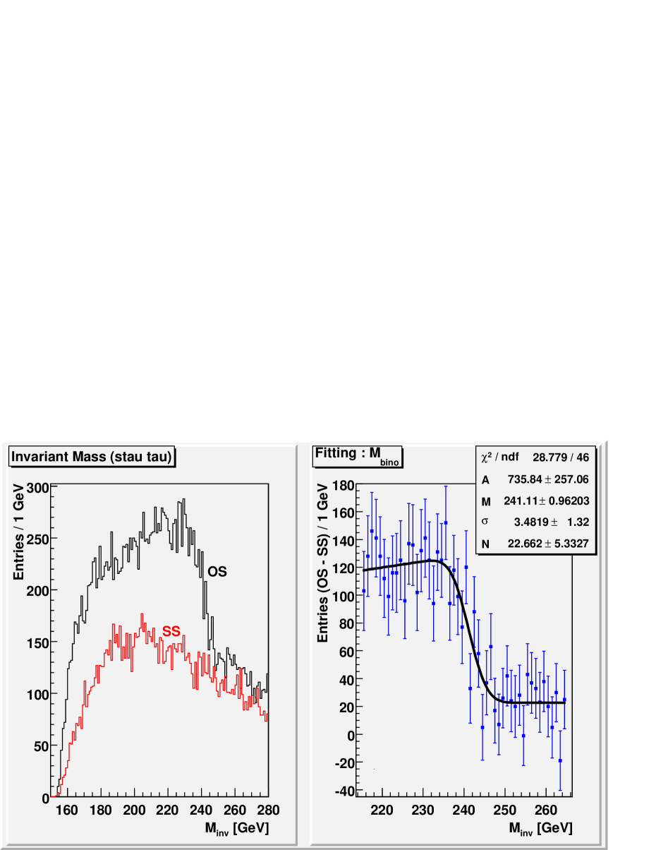
Figure 1: [Left]: The invariant mass distributions of opposite sign (black) and same sign (red) pairs for the GMSB case. Here, we take ${\cal L}=100\ {\rm fb}^{-1}$, and the postulated stau mass is taken to be the underlying value. [Right]: The fitting of the lightest neutralino mass after the charge subtraction.

By taking a difference between the OS and SS events, one can subtract the contributions from the backgrounds. The distribution of the signal events after the charge subtraction is shown in Fig. 1 (right). We can see a clearer endpoint. We search the upper endpoint by fitting the histogram with the Gaussian-smeared triangular function (including the effect of background) [24]:

$$\mbox{(Number of events)}=A\int_{-1}^{1}dz\exp\left[\frac{-1}{2\sigma^{2}}\left(M_{\tilde{\tau}_{1}j_{\tau}}-M^{\rm(max)}\sqrt{\frac{1+z}{2}}\right)^{2}\right]+N_{\rm BG},$$ (3.4)

where $A$, $M^{\rm(max)}$, $\sigma$, and $N_{\rm BG}$ are fitting parameters; in particular, $M^{\rm(max)}$ corresponds to the upper endpoint. The endpoint is determined to be $(241.11\pm 0.96)\ {\rm GeV}$, which is consistent with the underlying value of $m_{\chi^{0}_{1}}$.

In the above study, the charge subtraction method was very powerful in finding the neutralino endpoint. One can further try to find the second-lightest neutralino, which is almost the neutral Wino in this model. Although no clear endpoint can be seen in the OS events at $\sim m_{\chi^{0}_{2}}$, it shows up after the subtraction. (See Fig. 2, where the distribution of $M_{j_{\tau}\tilde{\tau}_{1}}$ is shown with the width of the bin of $5\ {\rm GeV}$.) By fitting the edge with the same function, $m_{\chi^{0}_{2}}$ is measured to be $(430.0\pm 4.5)\ {\rm GeV}$, which is slightly larger than the underlying value.

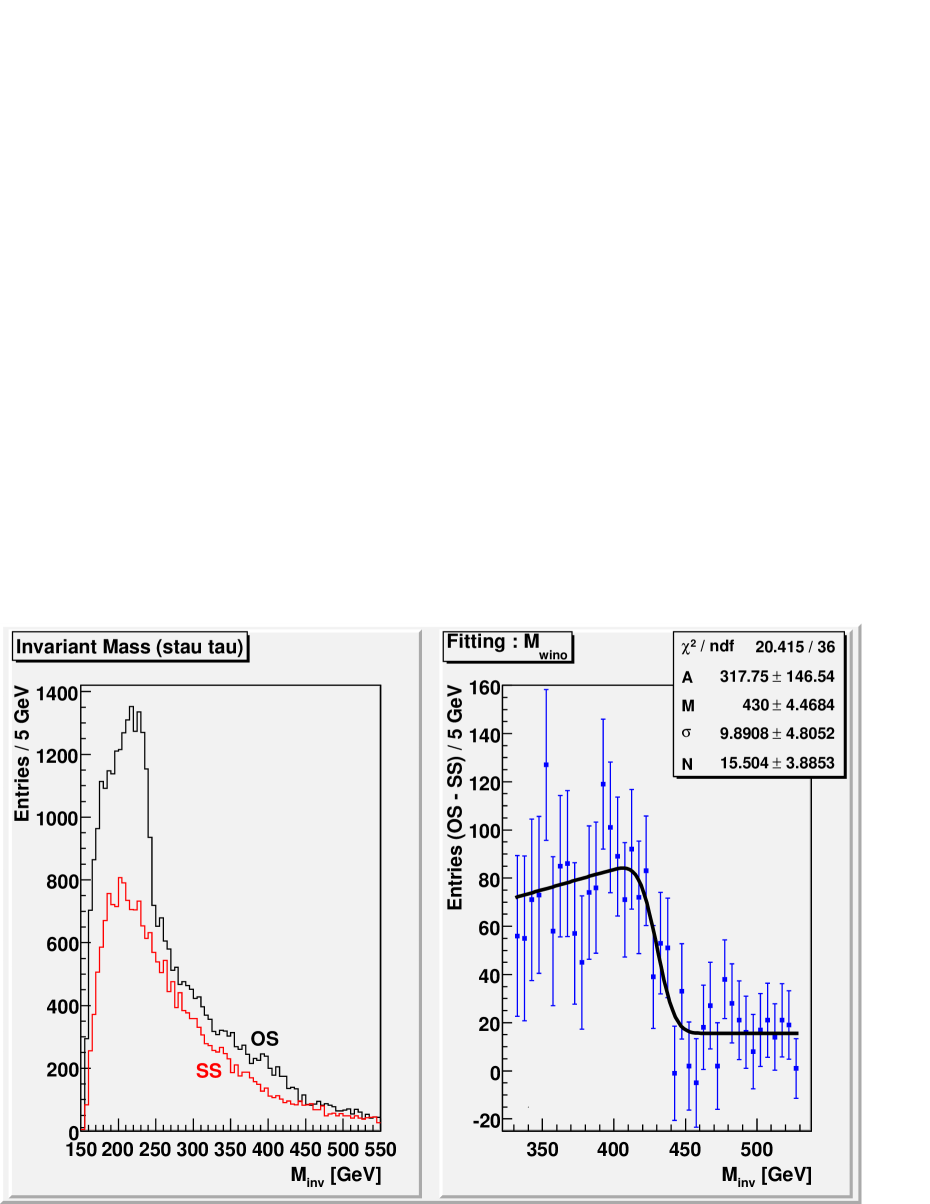
Figure 2: [Left]: The invariant mass distributions of opposite sign (black) and same sign (red) pairs for the GMSB case. Here, we take ${\cal L}=100\ {\rm fb}^{-1}$, and the width of the bin is $10\ {\rm GeV}$. [Right]: The fitting of the second-lightest neutralino mass after charge subtraction.

Before closing this subsection, we comment on the $m_{\tilde{\tau}_{1}}$-dependence of the reconstructed mass. The stau mass is expected to be measured in the long-lived stau scenario by combining the velocity and the momentum informations on the $\tilde{\tau}_{1}$ track; the expected error in the stau mass measurement is $\delta m_{\tilde{\tau}_{1}}\sim O(100\ {\rm MeV})$ [6, 7]. The neutralino mass measurements will therefore be affected by $O(100~{}{\rm MeV})$, which is less significant compared to the statistical uncertainties.

3.2 Slepton masses

We proceed to the discussion of the slepton mass measurements. In particular, it is interesting to measure the masses of $\tilde{e}_{R}$ and $\tilde{\mu}_{R}$ since one can learn the flavor structure of the model. Note that study of those particles are difficult in the Bino LSP scenario since they do not appear in the cascade decays. In order to measure $m_{\tilde{l}_{R}}$, we use the decay chain

$$\chi^{0}_{1}\rightarrow l^{\pm}\tilde{l}_{R}^{\mp}\rightarrow l^{\pm}l^{\mp}\tau\tilde{\tau}_{1},$$ (3.5)

followed by the hadronic decay of $\tau$. In the decay chain (3.5), the charges of $\tau$ and $\tilde{\tau}$ are opposite. We apply the following selections:

• At least one $\tilde{\tau}_{1}$ with the velocity $0.4\leq\beta_{\tilde{\tau}_{1}}\leq 0.9$.

• At least one $\tau$-tagged jet with $p_{T}>15\ {\rm GeV}$.

• At least one pair of isolated opposite-charge same-flavor leptons. We require $p_{T}>15\ {\rm GeV}$ for leptons.

For each event, we choose all the possible combinations of $(l^{+},l^{-},j_{\tau},\tilde{\tau}_{1})$ with requiring charges of $\tilde{\tau}_{1}$ and $j_{\tau}$ to be opposite. Assuming that $l^{+}$, $l^{-}$, $j_{\tau}$, and $\tilde{\tau}_{1}$ are all from the lightest neutralino whose mass is determined already, we can calculate the four-momentum of the $\tau$-lepton. Because the $\tau$-lepton from the slepton decay is usually ultra-relativistic, $\tau$ and $j_{\tau}$ are expected to be emitted to (almost) the same direction. The four-momentum of $\tau$ can thus be estimated as

$$p_{\tau}=z^{-1}p_{j_{\tau}},$$ (3.6)

where

$$z=\frac{2p_{j_{\tau}}\cdot(p_{l^{+}}+p_{l^{-}}+p_{\tilde{\tau}})}{\tilde{m}_{\chi^{0}_{1}}^{2}-(p_{l^{+}}+p_{l^{-}}+p_{\tilde{\tau}})^{2}},$$ (3.7)

with $\tilde{m}_{\chi^{0}_{1}}$ being the postulated value of the lightest neutralino mass for the analysis. The events with $z>1$ are rejected. In order to reconstruct the slepton mass $m_{\tilde{l}_{R}}$, we study the distribution of the following quantity:

$$M_{\tilde{l}}=\sqrt{(p_{l}+p_{\tilde{\tau}}+z^{-1}p_{j_{\tau}})^{2}}.$$ (3.8)

Here, $p_{l}$ is the four momentum of one of two charged leptons in $(l^{+},l^{-},j_{\tau},\tilde{\tau}_{1})$. Because we cannot tell which lepton is the one from the slepton decay, we calculate the invariant masses by using both of the possibilities.

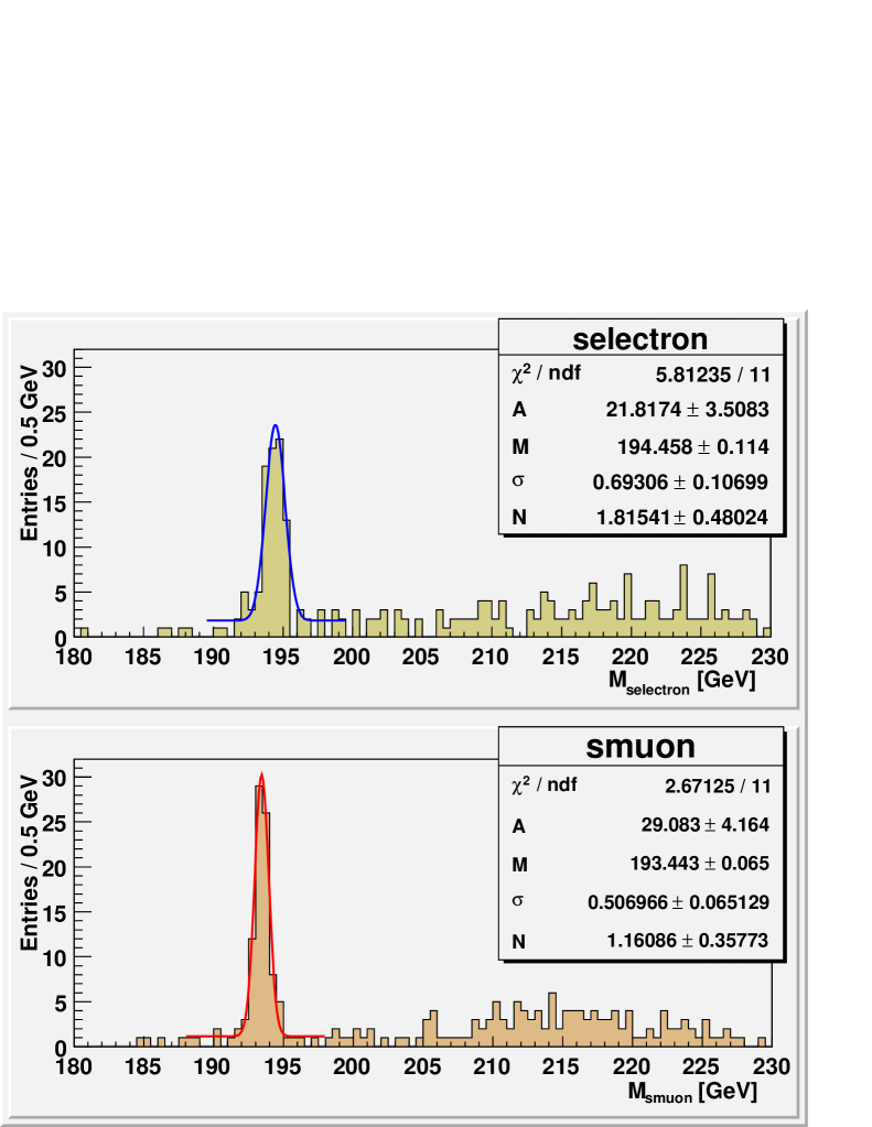
Figure 3: Distribution of $M_{\tilde{l}}$ with $l=e$ (left) and $\mu$ (right) for the GMSB case with ${\cal L}=100\ {\rm fb}^{-1}$. Here, the postulated stau and neutralino masses are chosen to be the underlying values.

In Fig. 3, we show the distributions of $M_{\tilde{l}}$ with $l=e$ and $\mu$. Here, the postulated values of the stau and the lightest neutralino masses are taken to be equal to the underlying values. Even though the distribution contains the combinatorial background, one can see sharp peaks at the slepton masses. Fitting the peaks with the Gaussian function plus a constant background,

$$\mbox{(Number of events)}=A\exp\left[-\frac{1}{2\sigma^{2}}\left(M_{\tilde{l}}-M^{\rm(peak)}\right)^{2}\right]+N_{\rm BG},$$ (3.9)

with $A$, $M^{\rm(peak)}$, $\sigma$, and $N_{\rm BG}$ being parameters, the peak positions $M^{\rm(peak)}$ are determined to be $(194.46\pm 0.11)~{}{\rm GeV}$ and $(193.44\pm 0.07)~{}{\rm GeV}$ for $l=e$ and $\mu$, respectively. Those values are in very good agreements with the actual slepton masses.

In the slepton mass determination, we should consider errors associated with the uncertainties in the mass measurements of stau and the lightest neutralino. In particular, the reconstructed slepton masses are sensitive to the uncertainty in the lightest neutralino mass. In Fig. 4, we show the reconstructed slepton masses (i.e., the 1-$\sigma$ upper and lower bounds with ${\cal L}=100\ {\rm fb}^{-1}$) as functions of the postulated lightest neutralino mass. One can see that the reconstructed slepton masses depend linearly on the postulated lightest neutralino mass. As mentioned in the previous section, the lightest neutralino mass can be measured by the endpoint study, and the uncertainty is $\sim 1\ {\rm GeV}$, which gives the error of $[\delta m_{\tilde{l}_{R}}]_{\delta m_{\chi^{0}_{1}}}\sim 1\ {\rm GeV}$ in the slepton mass measurement. Importantly, however, the mass difference $m_{\tilde{e}_{R}}-m_{\tilde{\mu}_{R}}$ is insensitive to the neutralino mass. The dependence of the reconstructed slepton masses on the postulated stau mass is proportional to $(m_{\chi^{0}_{1}}-m_{\tilde{l}_{R}})/m_{\chi^{0}_{1}}$, and thus rather weak in the present model.

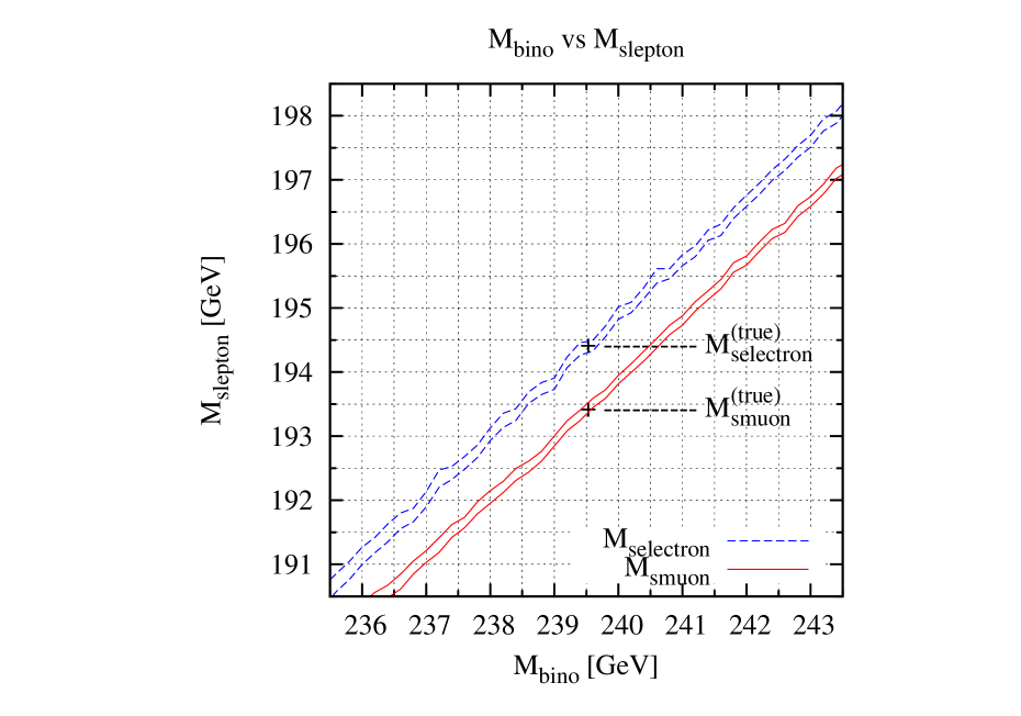
Figure 4: The reconstructed slepton masses as functions of the postulated lightest neutralino mass for the GMSB case.

3.3 Squark mass

Sqark masses can be also measured by reconstructing the decay chain:

$$\tilde{q}\rightarrow q\chi^{0}_{1}\rightarrow q\tau\tilde{\tau},$$ (3.10)

followed by hadronic decay of $\tau$. In order to use the decay chain (3.10), we adopt the following event selections:

• At least one $\tilde{\tau}_{1}$ with the velocity $0.4\leq\beta_{\tilde{\tau}_{1}}\leq 0.9$.

• At least one jet with $p_{T}>100\ {\rm GeV}$.

• At least one $\tau$-tagged jet with $p_{T}>15\ {\rm GeV}$.

• No isolated lepton with $p_{T}>15\ {\rm GeV}$.

The condition 3d) is to eliminate the mis-reconstruction of leptonically decaying $\tau$.

Then, we consider all the possible combinations $(j,j_{\tau},\tilde{\tau}_{1})$, where $j$ is one of four leading jets with $p_{T}>100\ {\rm GeV}$. Assuming that $j_{\tau}$ and $\tilde{\tau}_{1}$ are both from the decay of the neutralino, we first reconstruct the momentum of $\tau$, which is given by

$$p_{\tau}=z_{\tilde{q}}^{-1}p_{j_{\tau}},$$ (3.11)

where

$$z_{\tilde{q}}=\frac{2p_{j_{\tau}}\cdot p_{\tilde{\tau}}}{\tilde{m}_{\chi^{0}_{1}}^{2}-m_{\tilde{\tau}}^{2}}.$$ (3.12)

Combinations with $z_{\tilde{q}}>1$ is eliminated. Then, we study the distribution of the following variable:

$$M_{\tilde{q}}=\sqrt{(p_{j}+p_{\tilde{\tau}}+z_{\tilde{q}}^{-1}p_{j_{\tau}})^{2}}.$$ (3.13)

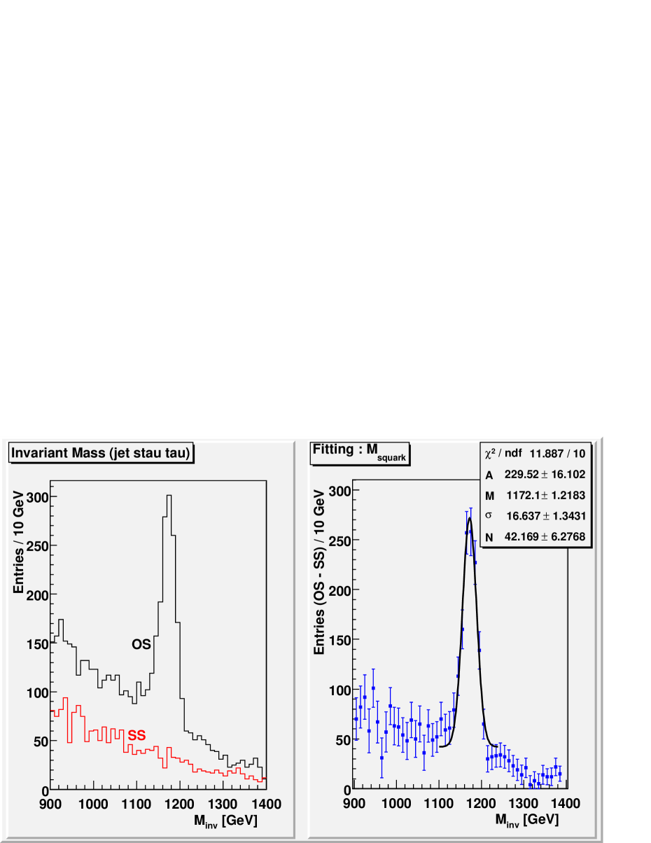
Figure 5: [Left]: The invariant mass distributions of opposite sign (black) and same sign (red) events. Here, we take ${\cal L}=100\ {\rm fb}^{-1}$, and the postulated stau mass is taken to be the underlying value of the stau mass. [Right]: The fit of the number of events with the Gaussian function.

The distribution of $M_{\tilde{q}}$ is shown in Figs. 5 for OS and SS events. We can see a clear peak for the OS event at the position corresponding to the squark masses, while no clear peak is seen for the SS event. By fitting the histogram after the charge subtraction with the Gaussian function, the peak position is obtained to be $m_{\tilde{q}}=(1172.1\ \pm 1.2)\ {\rm GeV}$, while underlying squark masses are $m_{\tilde{u}_{R}}=1184\ {\rm GeV}$, $m_{\tilde{d}_{R}}=1180\ {\rm GeV}$, $m_{\tilde{u}_{L}}=1232\ {\rm GeV}$, and $m_{\tilde{d}_{L}}=1234\ {\rm GeV}$. The dominant contribution to the histogram is from right-handed squarks. Compared to the right-handed squark masses, the observed peak location is smaller than the underlying values by $\sim 10\ {\rm GeV}$. It is partly from the mis-measurement of the jet energy and also from effects of the background. The uncertainties from the mis-measurements of the Bino and the stau masses are much smaller than the statistical error as far as the luminosity of ${\cal L}\sim 100\ {\rm fb}^{-1}$ is used.

In principle, a similar analysis can be performed by using the second-lightest neutralino (which is almost the Wino), which should provide information on the left-handed squark mass. However, the left-handed squarks decay into chargino (plus jet) as well as into neutralino. In addition, it is difficult to distinguish the left- and right-handed squark production events in the event-by-event basis. These become the source of extra background and reduce the signal-to-background ratio. Thus, for the study of the left-handed squark mass, we should perform more sophisticated analysis. A detailed discussion will be given elsewhere [25].

4 Implications

We have seen that, in the long-lived stau scenario, masses of various SUSY particles are expected to be measured with a very good accuracy at the LHC. This level of precise deterimnation of the mass spectrum may reveal the origin of SUSY breaking terms.

As we have seen, the masses of the lightest and the second-lightest neutralino, which almost correspond to the Bino and the neutral Wino, respectively, can be determined with the endpoint analyses. Then, combined with the gluino-mass information from, for example, the cross-section information for the process $pp\rightarrow\tilde{g}\tilde{g}$, we can test the GUT relation among the gaugino masses.

The masses of $\tilde{e}_{R}$ and $\tilde{\mu}_{R}$ are also measured with good accuracies. Even though the mass determinations of $\tilde{e}_{R}$ and $\tilde{\mu}_{R}$ are sensitive to the uncertainty in the lightest neutralino mass, the measured value of the mass differene $m_{\tilde{e}_{R}}-m_{\tilde{\mu}_{R}}$ is not affected to it. The mass difference $m_{\tilde{e}_{R}}-m_{\tilde{\mu}_{R}}$ contains various informations. Neglecting the flavor mixing, the slepton mass matrix has the form:

$${\cal M}^{2}_{\tilde{l}}=\left(\begin{array}[]{cc}m_{L}^{2}+\Delta_{\tilde{l},{LL}}&\Delta_{\tilde{l},{LR}}\\ \Delta_{\tilde{l},{LR}}&m_{R}^{2}+\Delta_{\tilde{l},{RR}}\end{array}\right),$$ (4.16)

where $m_{L}$ and $m_{R}$ are independent of the flavor index. Then, assuming that $\Delta\ll m_{L,R}^{2}$, the mass difference is given by

$$m_{\tilde{e}_{R}}-m_{\tilde{\mu}_{R}}\simeq\frac{1}{2m_{R}}(\Delta_{\tilde{e},{RR}}-\Delta_{\tilde{\mu},{RR}})-\frac{1}{2m_{R}(m_{L}^{2}-m_{R}^{2})}(\Delta_{\tilde{e},{LR}}^{2}-\Delta_{\tilde{\mu},{LR}}^{2}).$$ (4.17)

Thus, the slepton-mass difference is sensitive to the left-right mixing, whose information is in $\Delta_{\tilde{l},{LR}}$, as well as to the difference of the diagonal elements of the mass matrix. Even if the dominant contribution to the masses of sleptons (with the same gauge quantum numbers) is almost universal at some high energy scale, the universality is affected by various effects.

For example, in the GMSB models, the non-universality is originated from the supergravity effects and also from one-loop corrections with the muon Yukawa interaction. The supergravity effects are estimated as $\Delta_{\tilde{l},LL}\sim\Delta_{\tilde{l},RR}\sim O(m_{3/2}^{2})$, with $m_{3/2}$ being the gravitino mass. Thus, if the gravitino mass is as large as a few GeV, which is merginally consistent with the flavor-violation constraints depending on other SUSY parameters, the supergravity effect may be seen assuming that the mass difference $m_{\tilde{e}_{R}}-m_{\tilde{\mu}_{R}}$ is determined with the accuracy of $O(100\ {\rm MeV})$.

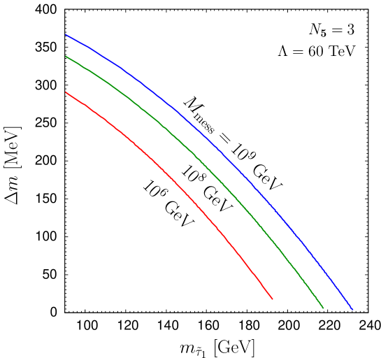
Figure 6: The selectron-smuon mass splitting calculated in the sweet-spot model.

The size of the loop effects is enhanced when $\tan\beta$ is large, and the contribution to the mass splitting is roughly estimated to be $O(100\ {\rm MeV})$ for $\tan\beta\gtrsim 30$. The actual value of the loop effects depends on the mechanism to generate the Higgs mass parameters since there is a one-loop diagram with Higgs fields in the loop. As an example of explicit models we calculate the mass splitting by solving renormalization group (RG) equations in the sweet-spot supersymmetry model [10]. SUSY breaking terms are determined by the parameters: $\Lambda$, $M_{\rm mess}$, $N_{\bf 5}$, and $\mu$. The Higgs mass parameters are generated at the unification scale rather than the messenger scale in this model, and hence there is a large logarithm in the quantum corrections. Also, the $\tan\beta$ parameter is predicted to be large due to the boundary condition at the messenger scale, $B=0$. The Yukawa coupling constants for the charged leptons are therfore enhanced. For these reasons, the mass splitting, $\Delta m\equiv m_{\tilde{e}_{R}}-m_{\tilde{\mu}_{R}}$, is expected to be large. Note also that for the same reason, $\tilde{\tau}_{1}$ can be significantly lighter than the other sleptons, that enables us to perform the analysis in the previous section.

The mass spectrum is calculated with fixing $\Lambda$ and $N_{\bf 5}$ as

$$\Lambda=60\ {\rm TeV},\ \ N_{\bf 5}=3,$$ (4.18)

so that the gaugino masses are similar to the ones in the example we took in the previous section. Since the value of $\mu$ (the Higgsino mass parameter) is strongly correlated to the stau mass in this model (through the RG effects mentioned above), we can trade the input parameter $\mu$ with $m_{\tilde{\tau}_{1}}$. We show in Fig. 6 the mass splitting as a function of the stau mass for various values of the messenger scale. For $M_{\rm mess}\gtrsim 10^{10}$ GeV, the slepton is heavier than the Bino with this set of parameters. The lines are terminated at the point where the stau becomes heavier than the other sleptons. One can see that the mass splitting can be as large as $\sim 300~{}{\rm MeV}$ which is large enough to be observed at the LHC. This calculation demonstrates that the mass splitting has a rich information on the microscopic theory to generate the SUSY breaking terms, especially those for the Higgs fields. It is also interesting to note that the LHC may be able to see an effect of the muon Yukawa coupling.

5 Conclusions

We have developed methods to measure the superparticle masses at the LHC in the long-lived stau scenario. We have concentrated on the scenario where $m_{\tilde{\tau}_{1}}<m_{\tilde{l}_{R}}<m_{\chi^{0}_{1}}$ (with $l=e$ and $\mu$) and demonstrated that the masses of neutralinos, sleptons and squarks can be well determined by endpoint or peak analysis.

In the neutralino mass measurements by the endpoint analysis of the $M_{j_{\tau}\tilde{\tau}}$ invariant masses, we have seen that the charge subtraction method is useful to identify the endpoints. In the sample point we have adopted, the estimated error in the lightest neutralino mass measurement is $\sim 1\ {\rm GeV}$. We have shown that even the second-lightest neutralino mass can be measured with an accuracy of $4-5\ {\rm GeV}$.

Once the lightest neutralino mass is known, it can be used to determine the masses of selectron and smuon. With the decay chain $\chi^{0}_{1}\rightarrow l^{\pm}\tilde{l}_{R}^{\mp}\rightarrow l^{\pm}l^{\mp}\tau\tilde{\tau}_{1}$, followed by hadronic decay of $\tau$, we first reconstruct the momentum of $\tau$ by using the relation $m_{\chi^{0}_{1}}=\sqrt{(p_{l^{+}}+p_{l^{-}}+p_{\tau}+p_{\tilde{\tau}})^{2}}$. Then, the slepton mass $m_{\tilde{l}_{R}}$ is determined in each event up to a combinatorics. With this method, we have seen that very sharp peaks are obtained around the underlying values of the slepton masses, which gives precise determination of the slepton masses. We have estimated the error in the slepton mass determination, which is $\sim 100\ {\rm MeV}$. Such a precise measurement of the slepton mass enables us to study effects of renormalization group, supergravity, and/or left-right mixing on the slepton masses. We also demonstrated that a sharp peak corresponding to (right-handed) squarks can be observed by using the $\tilde{q}\to q\chi_{1}^{0}\to q\tau\tilde{\tau}_{1}$ events.

Acknowledgments: We thank Prof. S. Asai for useful discussion. This work was supported in part by the Grant-in-Aid for Scientific Research from the Ministry of Education, Science, Sports, and Culture of Japan, no. 21840006 (R.K.) and no. 19540255 (T.M.).

References

- [1] M. Drees and X. Tata, Phys. Lett. B 252, 695 (1990).
- [2] J. L. Feng and T. Moroi, Phys. Rev. D 58, 035001 (1998).
- [3] S. P. Martin and J. D. Wells, Phys. Rev. D 59, 035008 (1999).
- [4] A. Nisati, S. Petrarca and G. Salvini, Mod. Phys. Lett. A 12, 2213 (1997).
- [5] G. Polesello and A. Rimoldi, ATLAS Internal Note ATL-MUON-99-006.
- [6] S. Ambrosanio, B. Mele, S. Petrarca, G. Polesello and A. Rimoldi, JHEP 0101, 014 (2001).
- [7] J. Ellis, A. R. Raklev and O. K. Oye, ATLAS Note ATL-PHYS-PUB-2007-016; ATLCOM- PHYS-2006-093.
- [8] I. Hinchliffe and F. E. Paige, Phys. Rev. D 60, 095002 (1999).
- [9] J. R. Ellis, A. R. Raklev and O. K. Oye, JHEP 0610, 061 (2006).
- [10] M. Ibe and R. Kitano, JHEP 0708, 016 (2007).
- [11] J. L. Feng, S. T. French, C. G. Lester, Y. Nir and Y. Shadmi, arXiv:0906.4215 [hep-ph]; J. L. Feng et al., arXiv:0910.1618 [hep-ph].
- [12] A. Rajaraman and B. T. Smith, Phys. Rev. D 76, 115004 (2007).
- [13] W. Buchmuller, K. Hamaguchi, M. Ratz and T. Yanagida, Phys. Lett. B 588, 90 (2004).
- [14] K. Hamaguchi, Y. Kuno, T. Nakaya and M. M. Nojiri, Phys. Rev. D 70, 115007 (2004).
- [15] J. L. Feng and B. T. Smith, Phys. Rev. D 71, 015004 (2005) [Erratum-ibid. D 71, 019904 (2005)].
- [16] K. Ishiwata, T. Ito and T. Moroi, Phys. Lett. B 669, 28 (2008).
- [17] R. Kitano, JHEP 0811, 045 (2008).
- [18] For the latest study, see M. Kawasaki, K. Kohri, T. Moroi and A. Yotsuyanagi, Phys. Rev. D 78, 065011 (2008).
- [19] F. E. Paige, S. D. Protopopescu, H. Baer and X. Tata, arXiv:hep-ph/0312045.
- [20] G. Corcella et al., JHEP 0101, 010 (2001); arXiv:hep-ph/0210213.
- [21] S. Moretti, K. Odagiri, P. Richardson, M. H. Seymour and B. R. Webber, JHEP 0204, 028 (2002).
-
[22]
For information on Pretty Good Simulation of high energy
collisions (PGS4), see
http://www.physics.ucdavis.edu/%7Econway/research/research.html. - [23] M. Dine, A. E. Nelson and Y. Shirman, Phys. Rev. D 51, 1362 (1995); M. Dine, A. E. Nelson, Y. Nir and Y. Shirman, Phys. Rev. D 53, 2658 (1996).
- [24] H. Bachacou, I. Hinchliffe and F. E. Paige, Phys. Rev. D 62, 015009 (2000).
- [25] T. Ito, R. Kitano and T. Moroi, in preparation.