Distributed Abstract Optimization via Constraints Consensus: Theory and Applications

Abstract

Distributed abstract programs are a novel class of distributed optimization problems where (i) the number of variables is much smaller than the number of constraints and (ii) each constraint is associated to a network node. Abstract optimization programs are a generalization of linear programs that captures numerous geometric optimization problems. We propose novel constraints consensus algorithms for distributed abstract programs: as each node iteratively identifies locally active constraints and exchanges them with its neighbors, the network computes the active constraints determining the global optimum. The proposed algorithms are appropriate for networks with weak time-dependent connectivity requirements and tight memory constraints. We show how suitable target localization and formation control problems can be tackled via constraints consensus.

I Introduction

This paper focuses on a class of distributed optimization problems and its application to target localization and formation control. Distributed optimization and computation have recently received widespread attention in the context of distributed estimation in sensor networks, distributed control of actuator networks and consensus algorithms. An early established reference on distributed optimization is [4], whereas a non-exhaustive set of recent references includes [5, 6, 7, 8]. We consider a distributed version of abstract optimization problems. Abstract optimization problems, sometimes referred to as abstract linear programs or as LP-type programs, generalize linear programming and model a variety of machine learning and geometric optimization problems. Examples of geometric optimization problems include the smallest enclosing ball, the smallest enclosing stripe and the smallest enclosing annulus problems. Early references to abstract optimization problems include [9, 10, 11]. In this paper we are interested in abstract optimization problems where the number of constraints $n$ is much greater than the number of constraints $\delta$ that identify the optimum solution (and where, therefore, there is a large number of redundant constraints). For example, we are interested in linear programs where $n$ is much greater than the number of variables $d$ (in linear programs, $\delta=d$). Under this dimensionality assumption, we consider distributed versions of abstract optimization programs, where $n$ is also the number of network nodes and where each constraint is associated to a node. We consider processor networks described by arbitrary, possibly time-dependent communication topologies and by computing nodes with tight memory constraints. After presenting and analyzing constraints consensus algorithms for distributed abstract optimization, we apply them to target localization in sensor networks and to formation control in robotic networks.

The relevant literature is vast; we organize it in three broad areas. First, linear programming and its generalizations, including abstract optimization, have received widespread attention in the literature. For linear programs in a fixed number of variables subject to $n$ linear inequalities, the earliest algorithm with time complexity in $O(n)$ is given in [12]. An efficient randomized algorithm is proposed in [9], where a linear program in $d$ variables subject to $n$ linear inequalities is solved in expected time $O(d^{2}n+e^{O(\sqrt{d\log d})})$; the expectation is taken over the internal randomizations executed by the algorithm. An elegant survey on randomized methods in linear programming and on abstract optimization is [13]; see also [11, 14]. The survey [15], see also [16], discusses the application of abstract optimization to a number of geometric optimization problems. Regarding parallel computation approaches to linear programming, linear programs with $n$ linear inequalities can be solved [17] by $n$ parallel processors in time $O((\log\log(n))^{d})$. However, the approach in [17], see also references therein, is limited to parallel random-access machines, where a shared memory is readable and writable to all processors. Other references on distributed linear programming include [18, 19].

A second relevant literature area is distributed training of support vector machines (SVMs). A randomized parallel algorithm for SVM training is proposed in [20] by using methods from abstract optimization and by exploiting the idea of exchanging only active constraints. Along these lines, [21] extends the algorithm to parallel computing over strongly connected networks, [22] contains a comprehensive discussion of SVM training via abstract optimization, and [23] applies similar algorithmic ideas to wireless sensor networks. The algorithms in [20, 21], independently developed at the same time of our works [1, 2, 3], differ from our constraint consensus algorithm in the following ways. First, the number of constraints stored at the nodes grows at each iteration so that both the memory and the local computation time at each node may be of order $n$. Second, our algorithm is proposed for general abstract optimization problems and thus may be applied to a variety of application domains. Third, our algorithm exploits a novel re-examination idea, is shown to be correct for time-varying (jointly strongly connected) digraphs, and features a distributed halting condition.

As third and final set of relevant references, we include a brief synopsis of recent progress in target localization in sensor networks and formation control in robotic networks. The problem of target localization has been widely investigated and recent interest has focused on sensors and wireless networks; e.g., see the recent text [24]. In this paper we take a deterministic worst-case approach to localization, adopting the set membership estimation technique proposed in [25]. A related sensor selection problem for target tracking is studied in [26]. Regarding the literature on formation control for robotic networks, an early reference on distributed algorithms and geometric patterns is [27]. Regarding the rendezvous problem, that is, the problem of gathering the robots at a common location, an early reference is [28]. The “circle formation control” problem, i.e., the problem of steering the robots to a circle formation, is discussed in [29]. The references [30, 31, 32] are based on, respectively, control-Lyapunov functions, input-to-state stability and cyclic pursuit.

The contributions of this paper are twofold. First, we identify and study distributed abstract programming as a novel class of distributed optimization problems that are tractable and widely applicable. We propose a novel algorithmic methodology, termed constraints consensus, to solve these problems in networks with various connectivity and memory constraints: as each node iteratively identifies locally active constraints and exchanges them with its neighbors, the globally active constraints determining the global optimum are collectively identified. A constraint re-examination idea is the distinctive detail of our algorithmic design. We propose three algorithms, a nominal one and two variations, to solve abstract programs depending on topology, memory and computation capabilities of the processor network. We formally establish various algorithm properties, including monotonicity, finite-time convergence to consensus, and convergence to the possibly-unique correct solution of the abstract program. Moreover, we provide a distributed halting conditions for the nominal algorithm. We provide a conservative upper bound on the completion time of the nominal algorithm and conjecture that the completion time depends linearly on $n$ (i.e., the number of constraints and the network dimension). Next, we evaluate the algorithm performance via a Monte Carlo probability-estimation analysis and we substantiate our conjecture on stochastically-generated sample problems. Sample problems are randomly generated by considering two classes of linear programs, taken from [33], and three types of graphs (line-graph, Erdős-Rènyi random graph and random geometric graph).

As a second set of contributions, we illustrate how distributed abstract programs are relevant for distributed target localization in sensor networks and for formation control problems, such as the rendezvous problem and the line or circle formation problems. Specifically, for the target localization problem, we design a distributed algorithm to estimate a convex polytope, specifically an axis-aligned bounding box, containing the moving target. Our proposed eight half-planes consensus algorithm combines (i) distributed linear programs to estimate the convex polytope at a given instant and (ii) a set-membership recursion, consisting of prediction and update steps, to dynamically track the region. We discuss correctness and memory complexity of the distributed estimation algorithm. Next, regarding formation control problems, we design a joint communication and motion coordination scheme for a robotic networks model involving range-based communication. We consider formations characterized by the geometric shapes of a point, a line, or a circle. We solve these formation control problems in a time-efficient distributed manner combining two algorithmic ideas: (i) the robots implement a constraints consensus algorithm to compute a common shape reachable in minimum-time, and (ii) the network connectivity is maintained by means of an appropriate standard connectivity-maintenance strategy. In the limit of vanishing robot displacement per communication round, our proposed move-to-consensus-shape strategy solves the optimal formation control tasks.

Paper organization

The paper is organized as follows. Section II introduces abstract optimization problems. Section III introduces network models. Section IV contains the definition of distributed abstract program and the constraints consensus algorithms. Section V contains the Monte Carlo analysis of the time-complexity of the constraints consensus algorithm. Sections VI and VII contain the application of the proposed constraints consensus algorithms to target localization and formation control.

Notation

We let ${\mathbb{Z}_{>0}}$, ${\mathbb{Z}_{\geq 0}}$, and ${\mathbb{R}}_{>0}$ denote the natural numbers, the non-negative integer numbers, and the positive real numbers, respectively. For $r\in{\mathbb{R}}_{>0}$ and $p\in{\mathbb{R}}^{d}$, we let $B(p,r)$ denote the closed ball centered at $p$ with radius $r$, that is, $B(p,r)=\{q\in{\mathbb{R}}^{d}\;|\;\|p-q\|_{2}\leq{r}\}$. For $d\in{\mathbb{Z}_{>0}}$, we ${0}_{d}$ and ${1}_{d}$ denote the vectors in ${\mathbb{R}}^{d}$ whose entries are all $0$ and $1$, respectively. Similarly, we let $\infty_{d}$ and $-\infty_{d}$ the vectors with $d$ entries $\infty$ and $-\infty$, respectively. For a finite set $A$, we let $\operatorname{card}(A)$ denote its cardinality. For two functions $f,g:{\mathbb{Z}_{>0}}\to{\mathbb{R}}_{>0}$, we write $f(n)\in O(g)$ (respectively, $f(n)\in\Omega(g)$) if there exist $N\in{\mathbb{Z}_{>0}}$ and $c\in{\mathbb{R}}_{>0}$ such that $f(n)\leq cg(n)$ for all $n\geq N$ (respectively, $f(n)\geq cg(n)$ for all $n\geq N$). Finally, we introduce the convention that sets are allowed to contain multiple copies of the same element.

Given $S\subset{\mathbb{R}}^{d}$ and $p\in{\mathbb{R}}^{d}$, let $\operatorname{dist}(p,S)$ denote the distance from $p$ to $S$, that is, $\operatorname{dist}(p,S)=\inf_{s\in S}\|p-s\|{}$. For distinct $p_{1}\in{\mathbb{R}}^{d}$ and $p_{2}\in{\mathbb{R}}^{d}$, let $\ell(p_{1},p_{2})$ be the line through $p_{1}$ and $p_{2}$. In what follows, a set of distinct points $\{p_{1},\dots,p_{n}\}\subset{\mathbb{R}}^{d}$, $n\geq 3$, is in stripe-generic position if, given any two ordered subsets $(p_{a},p_{b},p_{c})$ and $(p_{\alpha},p_{\beta},p_{\gamma})$, either $\operatorname{dist}(p_{a},\ell(p_{b},p_{c}))\neq\operatorname{dist}(p_{\alpha},\ell(p_{\beta},p_{\gamma}))$ or $(p_{a},p_{b},p_{c})=(p_{\alpha},p_{\beta},p_{\gamma})$.

II Abstract optimization

In this section we present an abstract framework [15, 14] that captures a wide class of optimization problems including linear programming and various machine learning and geometric optimization problems. Abstract optimization problems are also known as abstract linear programs, generalized linear programs or LP-type problems.

II-A Problem setup and examples

We consider optimization problems specified by a pair $(H,\phi)$, where $H$ is a finite set, and $\phi:2^{H}\rightarrow\Phi$ is a function with values in a linearly ordered set ($\Phi,\leq$); we assume that $\Phi$ has a minimum value $-\infty$. The elements of $H$ are called constraints, and for $G\subset H$, $\phi(G)$ is called the value of $G$. Intuitively, $\phi(G)$ is the smallest value attainable by a certain objective function while satisfying the constraints of $G$. An optimization problem of this sort is called an abstract optimization program if the following two axioms are satisfied:

1. Monotonicity: if $F\subset G\subset H$, then $\phi(F)\leq\phi(G)$;

2. Locality: if $F\subset G\subset H$ with $-\infty<\phi(F)=\phi(G)$, then, for all $h\in H$,

   $$\phi(G)<\phi(G\cup\{h\})\enspace\implies\enspace\phi(F)<\phi(F\cup\{h\}).$$

A set $B\subset H$ is minimal if $\phi(B)>\phi(B^{\prime})$ for all proper subsets $B^{\prime}$ of $B$. A minimal set $B$ with $-\infty<\phi(B)$ is a basis. Given $G\subset H$, a basis of $G$ is a minimal subset $B\subset G$, such that $-\infty<\phi(B)=\phi(G)$. A constraint $h$ is said to be violated by $G$, if $\phi(G)<\phi(G\cup\{h\})$.

A solution of an abstract optimization program $(H,\phi)$ is a minimal set $B_{H}\subset H$ with the property that $\phi(B_{H})=\phi(H)$. The combinatorial dimension $\delta$ of $(H,\phi)$ is the maximum cardinality of any basis. Finally, an abstract program is called basis regular if, for any basis with $\operatorname{card}(B)=\delta$ and any constraint $h\in H$, every basis of $B\cup\{h\}$ has the same cardinality of $B$. We now define two important primitive operations that are useful to solve abstract optimization problems:

1. Violation test: given a constraint $h$ and a basis $B$, it tests whether $h$ is violated by $B$; we denote this primitive by $\textup{{Viol}}(B,h)$;

2. Basis computation: given a constraint $h$ and a basis $B$, it computes a basis of $B\cup\{h\}$; we denote this primitive by $\textup{{Basis}}(B,h)$.

Example II.1 (Abstract framework for linear programs)

We recall from [13] how to transcribe a linear program into an abstract optimization program. A linear program (LP) in ${x\in{\mathbb{R}}^{d}}$ is given by

$$\begin{split}\min&\quad c^{T}x\\ \text{subject to}&\quad a_{i}^{T}x\leq b_{i},\quad i\in\{1,\dots,n\}\end{split}$$

where $d\in{\mathbb{Z}_{>0}}$ is the state dimension, $c\in{\mathbb{R}}^{d}$ characterizes the linear cost function to minimize, and $a_{i}\in{\mathbb{R}}^{d}$ and $b_{i}\in{\mathbb{R}}$ describe $n\in{\mathbb{Z}_{>0}}$ inequality constraints. In order to transcribe the LP into an abstract program, we need to specify the constraint set $H$ and the value $\phi(G)$ for each $G\subset H$. The constraint set $H$ is simply the set of half-spaces $\{h_{1},\ldots,h_{n}\}$, where $h_{i}=\{x\in{\mathbb{R}}^{d}\;|\;a_{i}^{T}x\leq b_{i}\}$. Defining the value function in order to satisfy the monotonicity and locality axioms is more delicate: if $\Phi=({\mathbb{R}},\leq)$ and $\phi(G)$ is the minimum of $c^{T}x$ subject to the constraint set $G$, then the locality axiom no longer holds (see Section 4 in [13] for a counterexample). A correct choice is as follows: let $(\Phi,\leq)$ be the set ${\mathbb{R}}^{d}$ with the lexicographical order, and define $\phi(G)=v_{G}$, where $v_{G}\in{\mathbb{R}}^{d}$ is the (unique) lexicographically minimal point $x$ minimizing $c^{T}x$ over the constraint set $G$, when it exists and is bounded. If the problem is infeasible (the intersection of the constraints in $G$ is empty), then $v_{G}=\infty_{d}$. If the problem is unbounded (no lexicographically minimal point exists), then $v_{G}=-\infty_{d}$. If $v_{G}$ is finite, then a basis of $G$ is a minimal subset of constraints $B\subset G$ such that $v_{B}=v_{G}$. It is known [9] that the abstract optimization program transcription of a feasible LP is basis regular and has combinatorial dimension $d$. A constraint $h\in H$ is violated by $G$ if and only if $v_{G}<v_{G\cup\{h\}}$. $\square$

Example II.2

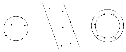
(Abstract optimization problems in geometric optimization) We present three useful geometric examples, illustrated in Figure 1.

1. Smallest enclosing ball: Given $n$ distinct points in ${\mathbb{R}}^{d}$, compute the center and radius of the ball of smallest volume containing all the points. This problem is [9] an abstract optimization program with combinatorial dimension $d+1$.

2. Smallest enclosing stripe: Given $n$ distinct points in ${\mathbb{R}}^{2}$ in stripe-generic positions, compute the center and the width of the stripe of smallest width containing all the points. In the Appendix we prove (for the first time at the best of our knowledge) that this problem is an abstract optimization program with combinatorial dimension $5$.

3. Smallest enclosing annulus: Given $n$ distinct points in ${\mathbb{R}}^{2}$, compute the center and the two radiuses of the annulus of smallest area containing all the points. This problem is [9] an abstract optimization program with combinatorial dimension $4$.

Figure 1: Smallest enclosing ball, stripe and annulus

In all three examples, the violation test and the basis computation primitives amount to low-dimensional geometric problems and are more or less straightforward. Numerous other geometric optimization problems can be cast as abstract optimization programs as discussed in [9, 10, 13, 15] $\square$

We end this section with a useful lemma, that is an immediate consequence of locality, and a useful rare property.

Lemma II.3

For any $F$ and $G$ subsets of $H$, $\phi(F\cup{G})>\phi(F)$ if and only if there exists $g\in{G}$ such that $\phi(F\cup\{g\})>\phi(F)$.

Proof.

If there exists $g\in{G}$ such that $\phi(F\cup\{g\})>\phi(F)$, then by monotonicity $\phi(F\cup{G})\geq\phi(F\cup\{g\})>\phi(F)$. For the other implication, assume $G=\{g_{1},\ldots,g_{k}\}$ for some $k\in{\mathbb{Z}_{>0}}$, and define $G_{i}:=\{g_{1},\ldots,g_{i}\}$ for $i\in\{1,\dots,k\}$. We may rewrite the assumption $\phi(F\cup{G})>\phi(F)$ as $\phi(F\cup G_{k-1}\cup\{g_{k}\})>\phi(F)$. If $\phi(F\cup G_{k-1})=\phi(F)$, then the locality axiom implies $\phi(F\cup\{g_{k}\})>\phi(F)$ and the thesis follows with $g=g_{k}$. Otherwise, the same argument may be applied to $G_{k-1}$. The recursion stops either when $\phi(F\cup{G_{i}})=\phi(F)$ (and the thesis follows with $g=g_{i+1}$) for some $i$ or when $\phi(F\cup G_{1})>\phi(F)$ (and the thesis follows with $g=g_{1}$). ∎

Next, given an abstract optimization program $(H,\omega)$, let $B_{G}$ denote the basis of any $G\subseteq H$. An element $h$ of $B_{H}$ is persistent if $h\in B_{G}$ for all $G\subseteq H$ containing $h$. An abstract optimization program $(H,\omega)$ is persistent if all elements of $B_{H}$ are persistent. The persistence property is useful, as we state in the following result.

Lemma II.4

Any persistent abstract optimization program $(H,\omega)$ can be solved in a number of time steps equal to the dimension of $H$.

Proof.

Let $H=\{h_{1},\ldots,h_{n}\}$. Set $B=\{h_{1},\ldots,h_{\delta}\}$ and then update $B=\textup{{Basis}}(B,h_{k})$ for $k=\delta+1,\ldots,n$. Because of persistency, each $h\in B_{H}$ is added to $B$ once it is selected as $h_{k}$ and is not removed from $B$ in subsequent basis computations. ∎

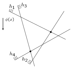
Unfortunately, the persistence property is rare. Indeed, in Figure 2 we show an LP problem where the persistency property does not hold. In fact, it can be easily noticed that $\{h_{1},h_{2}\}$ is a basis for $\{h_{1},h_{2},h_{3},h_{4}\}$, but $\{h_{3},h_{4}\}$ is a basis for $\{h_{2},h_{3},h_{4}\}$. In other words $\{h_{2}\}$ is not violated by $\{h_{3},h_{4}\}$. The lack of persistency complicates the design of centralized and distributed solvers for abstract optimization problems. For example, in network settings, flooding algorithms are not sufficient.

Figure 2: An LP problem that is not persistent.

II-B Randomized sub-exponential algorithm

In the following sections we will assume that each node in the network possesses a routine capable of solving small-dimensional abstract optimization programs. For completeness’ sake, this section reviews the randomized algorithm proposed in [9]. This algorithm has expected running time with linear dependence on the number of constraints, whenever the combinatorial dimension $\delta$ is fixed, and with sub-exponential dependence on the $\delta$; these bounds are proven in [9] for linear programs and in [13] for general abstract optimization programs. The algorithm, called Subex_LP, has a recursive structure and is based on the violation test and the basis computation primitives. Given a set of constraints $G$ and a candidate basis $C\subset G$, the algorithm is stated as follows:

function $\textup{{Subex\_LP}}(G,C)$

1:  if $G=C$, then return $C$

2:  else

3:   choose a random $h\in G\setminus C$ and compute $B:=\textup{{Subex\_LP}}(G\setminus\{h\},C)$

4:   if $\textup{{Viol}}(B,h)$ (that is, $h$ is violated by $B$), then

5:    compute $B^{\prime}:=$ basis for $B\cup\{h\}$

6:    return $\textup{{Subex\_LP}}(G,\textup{{Basis}}(B,h))$

7:   else return $B$

8:   endif

9:  endif

For the abstract optimization program $(H,\phi)$, the routine is invoked with $\textup{{Subex\_LP}}(H,B)$, given any initial candidate basis $B$.

III Network models

Following [34], we define a synchronous network system as a “collection of computing elements located at nodes of a directed network graph.” We refer to computing elements are processors.

III-A Digraphs and connectivity

We let $\mathcal{G}=(\{1,\dots,n\},E)$ denote a directed graph (or digraph), where $\{1,\dots,n\}$ is the set of nodes and $E\subset\{1,\dots,n\}^{2}$ is the set of edges. For each node $i$ of $\mathcal{G}$, the number of edges going out from (resp. coming into) node $i$ is called out-degree (resp. in-degree). A digraph is strongly connected if, for every pair of nodes $(i,j)\in\{1,\dots,n\}\times\{1,\dots,n\}$, there exists a path of directed edges that goes from $i$ to $j$. A digraph is weakly connected if replacing all its directed edges with undirected edges results in a connected undirected graph. In a strongly connected digraph, the minimum number of edges between node $i$ and $j$ is called the distance from $i$ to $j$ and is denoted $\operatorname{dist}(i,j)$. The maximum $\operatorname{dist}(i,j)$ taken over all pairs $(i,j)$ is the diameter and is denoted $\operatorname{diam}(\mathcal{G})$. Finally, we consider time-dependent digraphs of the form $t\mapsto\mathcal{G}(t)=(\{1,\dots,n\},E(t))$. The time-dependent digraph $\mathcal{G}$ is jointly strongly connected if, for every $t\in{\mathbb{Z}_{\geq 0}}$, the digraph $\cup_{\tau=t}^{+\infty}\mathcal{G}(\tau)$ is strongly connected.

In a time-dependent digraph, the set of outgoing (incoming) neighbors of node $i$ at time $t$ are the set of nodes to (from) which there are edges from (to) $i$ at time $t$. They are denoted by ${\mathcal{N}}_{\textup{out}}(i,t)$ and ${\mathcal{N}}_{\textup{in}}(i,t)$, respectively.

III-B Synchronous networks and distributed algorithms

A synchronous network is a time-dependent digraph $\mathcal{G}=(\{1,\dots,n\},{E}_{\textup{cmm}})$, where $\{1,\dots,n\}$ is the set of identifiers of the processors, and the time-dependent set of edges ${E}_{\textup{cmm}}$ describes communication among processors as follows: $(i,j)$ is in ${E}_{\textup{cmm}}(t)$ if and only if processor $i$ can communicate to processor $j$ at time $t\in{\mathbb{Z}_{\geq 0}}$.

For a synchronous network $\mathcal{G}$ with processors $\{1,\dots,n\}$, a distributed algorithm consists of (1) the set $W$, called the set of processor states ${w}^{[i]}$, for all $i\in\{1,\dots,n\}$; (2) the set $\mathbb{A}$, called the message alphabet, including the null symbol; (3) the map $\textup{msg}:W\times\{1,\dots,n\}\rightarrow\mathbb{A}$, called the message-generation function; and (4) the map $\textup{stf}:W\times\mathbb{A}^{n}\rightarrow W$, called the state-transition function. The execution of the distributed algorithm by the network begins with all processors in their start states. The processors repeatedly perform the following two actions. First, the $i$th processor sends to each of its outgoing neighbors in the communication graph a message (possibly the null message) computed by applying the message-generation function to the current value of ${w}^{[i]}$. After a negligible period of time, the $i$th processor computes the new value of its processor state ${w}^{[i]}$ by applying the state-transition function to the current value of ${w}^{[i]}$, and to the incoming messages (present in each communication edge). The combination of the two actions is called a communication round or simply a round.

In this execution scheme we have assumed that each processor executes all the calculations in one round. If it is not possible to upper bound the execution-time of the algorithm, then one may consider a slightly different network model that allows the state-transition function to be executed across multiple rounds. When this happens, the message is generated by using the processor state at the previous round.

The last aspect to consider is the algorithm halting, that is a situation such that the network (and therefore each processor) is in a idle mode. Such status can be used to indicate the achievement of a prescribed task. Formally we say that a distributed algorithm is in halting status if the processor state is a fixed point for the state-transition function (that becomes a self-loop) and no message (or equivalently the null message) is generated at each node.

IV Distributed abstract optimization

In this section we define distributed abstract programs, propose novel distributed algorithms for their solutions and analyze their correctness.

IV-A Problem statement

Informally, a distributed abstract program consists of three main elements: a network, an abstract optimization program and a mechanism to distribute the constraints of the abstract program among the nodes of the network.

Definition IV.1

A distributed abstract program is a tuple $(\mathcal{G},(H,\phi),\mathcal{B})$ consisting of

1. $\mathcal{G}=(\{1,\dots,n\},{E}_{\textup{cmm}})$, a synchronous network;

2. $(H,\phi)$, an abstract program; and

3. $\mathcal{B}:H\rightarrow\{1,\dots,n\}$, a surjective map called constraint distribution map that associates to each constraint one network node.

If the map $\mathcal{B}$ is a bijection, we denote the distributed abstract program with the pair $(\mathcal{G},(H,\phi))$. A solution of $(\mathcal{G},(H,\phi),\mathcal{B})$ is attained when all network processors have computed a solution to $(H,\phi)$.

Remark IV.2

The most natural choice of constraint distribution map $\mathcal{B}$ is a bijection; in this case, (i) the network dimension is equal to the dimension of the abstract optimization program and (ii) precisely one constraint is assigned to each network node. More complex distribution maps are interesting depending on the computation power and memory of the network processors. In what follows, we typically assume $\mathcal{B}$ to be a bijection. $\square$

IV-B Constraints consensus algorithms

Here we propose three novel distributed algorithms that solve distributed abstract programs. First, we describe a distributed algorithm that is well-suited for time-dependent networks whose nodes have bounded computation time, memory and in-degree. Equivalently, the algorithm is applicable to networks with arbitrary in-degree, but also arbitrary computation time and memory. Then we describe two variations that deal with arbitrary in-degree versus short computation time and small memory. The second version of the algorithm is well-suited for time-dependent networks that have arbitrary in-degree and bounded computation time, but also arbitrary memory (in the sense that the number of stored messages may depend on the number of nodes of the network). The third algorithm considers the case of time-independent networks with arbitrary in-degree and bounded computation time and memory.

In all algorithms we consider a synchronous network $\mathcal{G}$ and an abstract program $(H,\phi)$ with $H=\{h_{1},\cdots,h_{n}\}$ and with combinatorial dimension $\delta$. We define a distributed abstract program by assuming that constraints and nodes are in a one-to-one relationship, and we let $h_{i}$ be the constraint associated with network node $i$. Here is an informal description of our first algorithm.

Constraints Consensus Algorithm: Beside having access to the constraint $h_{i}$, the $i$th processor state contains a candidate basis ${B}^{[i]}$ consisting of $\delta$ elements of $H$. The processor state ${B}^{[i]}$ is initialized to $\delta$ copies of $h_{i}$. At each communication round, the processor performs the following tasks: (i) it transmits ${B}^{[i]}$ to its out-neighbors and acquires from its in-neighbors their candidate bases; (ii) it solves an abstract optimization program with constraint set given by the union of: its constraint $h_{i}$, its candidate basis ${B}^{[i]}$ and its in-neighbors’ candidate bases; (iii) it updates ${B}^{[i]}$ to be the solution of the abstract program computed at step (ii).

For completeness’ sake, the following table presents the algorithm in a way that is compatible with the model given in Section III-B. The Subex_LP algorithm is adopted as local solver for abstract optimization programs.

 

Problem data:

$(\mathcal{G},(H,\phi))$

Algorithm:

Constraints Consensus

Message alphabet:

$\mathbb{A}=H^{\delta}\cup\{\textup{{null}}\}$

Processor state:

${B}^{[i]}\subset H$ with $\operatorname{card}({B}^{[i]})=\delta$

Initialization:

${B}^{[i]}:=\{h_{i},\dots,h_{i}\}$

function $\textup{msg}({B}^{[i]},j)$

1:  return ${B}^{[i]}$

function $\textup{stf}({B}^{[i]},y)$
% executed by node $i$, with $y_{j}:=\textup{msg}({B}^{[j]},i)={B}^{[j]}$

1:  ${H}_{\textup{tmp}}:=\{h_{i}\}\cup{B}^{[i]}\cup\big{(}\cup_{j\in{\mathcal{N}}_{\textup{in}}(i)}y_{j}\big{)}$

2:  return $\textup{{Subex\_LP}}({H}_{\textup{tmp}},{B}^{[i]})$

 

Remark IV.3

(Constraint re-examination due to lack of persistency) In order for the algorithm to compute a correct solution, it is necessary that each node continuously re-examine its associated constraint throughout algorithm execution. In other words, step 1: of the state-transition function stf in the algorithm may not be replaced by ${H}_{\textup{tmp}}:={B}^{[i]}\cup\big{(}\cup_{j\in{\mathcal{N}}_{\textup{in}}(i)}y_{j}\big{)}$. This continuous re-examination is required because of the lack of the persistency property discussed after Lemma II.4. $\square$

In the second scenario we consider a time-dependent network with no bounds on the in-degree of the nodes and on the memory size. In this setting the execution of the Subex_LP may exceed the computation time allocated between communication rounds. To deal with this problem, we introduce an “asynchronous” version of the network model described in Section III: we allow a processor to execute message-transmission and state-transition functions at instants that are not necessarily synchronized. Here is an informal description of the algorithm.

Multi-round constraints consensus algorithm Each processor has the same message alphabet, processor state, and initialization settings as in the previous constraints consensus algorithm. The processor performs two tasks in parallel. Task #1: at each communication round, the processor transmits to its out-neighbors its candidate basis ${B}^{[i]}$ and acquires from its in-neighbors their candidate bases. Task #2: independently of communication rounds, the processor repeatedly solves an abstract optimization program with constraint set given by the union of: its constraint $h_{i}$, its candidate basis ${B}^{[i]}$ and its in-neighbors’ candidate bases; the solution of this abstract program becomes the new candidate basis ${B}^{[i]}$. The abstract program solver is invoked with the most-recently available in-neighbors’ candidate bases and, throughout its execution, this information does not change.

In the third scenario we consider a time-independent network with no bounds on the in-degree of the nodes. We suppose that each processor has limited memory capacity, so that it can store at most $D$ constraints in $H$. The memory is dimensioned so as to guarantee that the abstract optimization program is always solvable during two communication rounds (e.g., by adopting the Subex_LP solver). The memory constraint is dealt with by processing only part of the incoming messages at each round, and by cycling among incoming messages in such a way as to process all the messages in multiple rounds.

Cycling constraints consensus algorithm The processor state contains and initializes a candidate basis ${B}^{[i]}$ as in the basic constraints consensus algorithm. Additionally, the processor state includes a counter variable that keeps track of communication rounds. At each communication round, the processor performs the following tasks: (i) it transmits ${B}^{[i]}$ to its out-neighbors and receives from its in-neighbors their candidate bases; (ii) among the incoming messages, it chooses to store $D$ messages according to a scheduled protocol and the counter variable; (iii) it solves an abstract optimization program with constraint set given by the union of: its constraint $h_{i}$, its candidate basis ${B}^{[i]}$ and the $D$ candidate bases from its in-neighbors; (iv) it updates ${B}^{[i]}$ to be the solution of the abstract program computed at step (iii).

IV-C Algorithm analysis

We are now ready to analyze the algorithms. In what follows, we discuss correctness, halting conditions, memory complexity and time complexity.

Theorem IV.4

(Correctness of the constraints consensus algorithm) Let $(\mathcal{G},(H,\phi))$ be a distributed abstract program with nodes and constraints in one-to-one relationship. Assume the time-dependent network $\mathcal{G}$ is jointly strongly connected. Consider a constraint consensus algorithm in which a network node initializes its candidate basis to a constraint set with finite value. The following statements hold:

1. along the evolution of the constraints consensus algorithm, the basis value $t\mapsto\phi({B}^{[i]}(t))$ at each node $i\in\{1,\dots,n\}$ is monotonically non-decreasing and converges to a constant finite value in finite time;

2. the constraints consensus algorithm solves the distributed abstract program $(\mathcal{G},(H,\phi))$, that is, in finite time the candidate basis ${B}^{[i]}$ at each node $i$ is a solution of $(H,\phi)$; and

3. if the distributed abstract program has a unique minimal basis $B_{H}$, then the final candidate basis ${B}^{[i]}$ at each node $i$ is equal to $B_{H}$.

Proof.

From the monotonicity axiom of abstract optimization and from the finiteness of $H$, it follows that each sequence $\phi({B}^{[i]}(t))$, $t\in{\mathbb{Z}_{\geq 0}}$, is monotone non-decreasing, upper bounded and can assume only a finite number of values. Additionally, in finite time, each node has a candidate basis that has finite value because, by assumption, one node starts with a candidate basis with finite value and the digraph is jointly strongly connected. Therefore, the constraints consensus algorithm at every node converges to a constant candidate basis with finite value in a finite number of steps. This concludes the proof of fact (i). In what follows, let ${B}^{[1]},\dots,{B}^{[n]}$ denote the limiting candidate bases at each node in the graph.

We prove fact (ii) in three steps. First, we proceed by contradiction to prove that all the nodes converge to the same value (but not necessarily the same basis). The following fact is known: if a time-dependent digraph is jointly strongly connected, then the digraph contains a time-dependent directed path from any node to any other node beginning at any time, that is, for each $t\in{\mathbb{Z}_{\geq 0}}$ and each pair $(i,j)$, there exists a sequence of nodes $\ell_{1},\dots,\ell_{k}$ and a sequence of time instants $t_{1},\dots,t_{k+1}\in{\mathbb{Z}_{\geq 0}}$ with $t\leq t_{1}<\dots<t_{k+1}$, such that the directed edges $\{(i,\ell_{1}),(\ell_{1},\ell_{2}),\dots,(\ell_{k},j)\}$ belong to the digraph at time instants $\{t_{1},\dots,t_{k+1}\}$, respectively. The proof by contradiction of a closely related fact is given in [35, Theorem 9.3]. Now, suppose that at time $t_{0}$ all the nodes have converged to their limit bases and that there exist at least two nodes, say $i$ and $j$, such that $\phi({B}^{[i]})\neq\phi({B}^{[j]})$. For $t=t_{0}+1$, for every $k_{1}\in{\mathcal{N}}_{\textup{out}}(i,t_{0}+1)$, no constraint in ${B}^{[i]}$ violates ${B}^{[k_{1}]}$, otherwise node $k_{1}$ would compute a new distinct basis with strictly larger value, thus violating the assumption that all nodes have converged. Therefore, $\phi({B}^{[i]})\leq\phi({B}^{[k_{1}]})$. Using the same argument at $t=t_{0}+2$, for every $k_{2}\in{\mathcal{N}}_{\textup{out}}(k_{1},t_{0}+2)$, no constraint in ${B}^{[k_{1}]}$ violates ${B}^{[k_{2}]}$. Therefore, $\phi({B}^{[i]})\leq\phi({B}^{[k_{1}]})\leq\phi({B}^{[k_{2}]})$. Iterating this argument, we can show that for every $S>0$, every node $k$, that is reachable from $i$ in the time-dependent digraph with a time-dependent directed path of length at most $S$, has a basis ${B}^{[k]}$ such that $\phi({B}^{[i]})\leq\phi({B}^{[k]})$. However, because the digraph is jointly strongly connected, we know that there exists a time-dependent directed path from node $i$ to node $j$ beginning at time $t_{0}$, thus showing that $\phi({B}^{[i]})\leq\phi({B}^{[j]})$. Repeating the same argument by starting from node $j$ we obtain that $\phi({B}^{[j]})\leq\phi({B}^{[i]})$. In summary, we showed that $\phi({B}^{[i]})=\phi({B}^{[j]})$, thus giving the contradiction. Note that this argument also proves that, if $(i,j)$ is an edge of the digraph $\cup_{\tau=t}^{+\infty}\mathcal{G}(\tau)$, then no constraint in $i$ violates ${B}^{[j]}$ and, therefore, $\phi({B}^{[i]}\cup{B}^{[j]})=\phi({B}^{[j]})$. Also, the equality ${B}^{[i]}\cup{B}^{[j]}={B}^{[j]}\cup{B}^{[i]}$ implies that there exists $\bar{\phi}\in{\mathbb{R}}$ such that $\bar{\phi}=\phi({B}^{[i]})=\phi({B}^{[j]})=\phi({B}^{[i]}\cup{B}^{[j]})=\phi({B}^{[j]}\cup{B}^{[i]})$ for all $i\in\{1,\dots,n\}$ and $(i,j)$ edges of $\cup_{\tau=t}^{+\infty}\mathcal{G}(\tau)$.

Second, we claim that the value of the basis at each node is equal to the value of the union of all the bases. In other words, we claim that

$$\bar{\phi}=\phi({B}^{[1]}\cup\cdots\cup{B}^{[n]}).$$ (1)

We prove equation (1) by induction. First, we note that $\bar{\phi}=\phi({B}^{[i]}\cup{B}^{[j]})$ for any nodes $i$ and $j$ such that either $(i,j)$ or $(j,i)$ is a directed edge in $\cup_{\tau=t}^{+\infty}\mathcal{G}(\tau)$. Without loss of generality, let us assume $i=1$ and $j=2$. Now assume that

$$\phi({B}^{[1]}\cup\cdots\cup{B}^{[k]})=\bar{\phi},$$ (2)

for an arbitrary $k$-dimensional weakly-connected subgraph $G_{k}$ of $\cup_{\tau=t}^{+\infty}\mathcal{G}(\tau)$ and we prove such a statement for a weakly-connected subgraph of dimension $k+1$ containing $G_{k}$. By contradiction, we assume the statement is not true for $k+1$. Assuming, without loss of generality, that node $k+1$ is connected to $G_{k}$ in $\cup_{\tau=t}^{+\infty}\mathcal{G}(\tau)$, we aim to find a contradiction with the statement

$$\phi({B}^{[1]}\cup\cdots\cup{B}^{[k]}\cup{B}^{[k+1]})>\bar{\phi}.$$ (3)

Plugging the induction assumption into equation (3), we have

$$\phi({B}^{[1]}\cup\cdots\cup{B}^{[k]}\cup{B}^{[k+1]})>\phi({B}^{[1]}\cup\cdots\cup{B}^{[k]}).$$ (4)

From Lemma II.3 with $F={B}^{[1]}\cup\cdots\cup{B}^{[k]}$ and $G={B}^{[k+1]}$ and noting equation (4), we conclude that there exists $g\in{B}^{[k+1]}$ such that

$$\phi({B}^{[1]}\cup\cdots\cup{B}^{[k]}\cup\{g\})>\phi({B}^{[1]}\cup\cdots\cup{B}^{[k]}).$$ (5)

Next, select a node $p\in\{1,\dots,k\}$ such that either $(p,k+1)$ or $(k+1,p)$ is a directed edge of $\cup_{\tau=t}^{+\infty}\mathcal{G}(\tau)$ and note that ${B}^{[p]}\subset{B}^{[1]}\cup\cdots\cup{B}^{[k]}$ and $\phi({B}^{[p]})=\phi({B}^{[1]}\cup\cdots\cup{B}^{[k]})$ by the induction assumption. From these two facts together with equation (5), the locality property implies that

$$\phi({B}^{[p]}\cup\{g\})>\phi({B}^{[p]}).$$ (6)

Finally, the contradiction follows by noting:

$$\phi({B}^{[p]}) \overset{\text{bases have converged}}{=}\phi({B}^{[p]}\cup{B}^{[k+1]})\overset{\text{monotonicity}}{\geq}\phi({B}^{[p]}\cup\{g\})\overset{\text{by equation}~{}\eqref{eq:four}}{>}\phi({B}^{[p]}).$$

This concludes the proof of equation (1).

Third and final, because no constraint in $\{h_{1},\ldots,h_{n}\}$ violates the set ${B}^{[1]}\cup\cdots\cup{B}^{[n]}$ and because ${B}^{[1]}\cup\cdots\cup{B}^{[n]}\subset H$, Lemma II.3 and equation (1) together imply

$$\bar{\phi}=\phi({B}^{[1]}\cup\cdots\cup{B}^{[n]})=\phi(H).$$

This equality proves that in a finite number of rounds the candidate basis at each node is a solution to $(H,\phi)$ and, therefore, this concludes our proof of fact (ii). The proof of fact (iii) is straightforward. ∎

Remark IV.5

(Correctness of multi-round and cycling constraints consensus) Correctness of the other two versions of the constraints consensus algorithm may be established along the same lines. For example, it is immediate to establish that the basis at each node reaches a constant value in finite time. It is easy to show that this constant value is the solution of the abstract optimization program for the multi-round algorithm over a time-dependent graph. For the cycling algorithm over a time-independent graph we note that the procedure used to process the incoming data is equivalent to considering a time-dependent graph whose edges change with that law. $\square$

Theorem IV.6 (Halting condition)

Consider a network described by a time-independent strongly-connected digraph $\mathcal{G}$ implementing a constraints consensus algorithm in which a network node initializes its candidate basis to a constraint set with finite value. Each processor can halt the algorithm execution if the value of its basis has not changed after $2\operatorname{diam}(\mathcal{G})+1$ communication rounds.

Proof.

For all $t\in{\mathbb{Z}_{\geq 0}}$ and for every $(i,j)$ edge of $\mathcal{G}$,

$$\phi({B}^{[i]}(t))\leq\phi({B}^{[j]}(t+1)),$$ (7)

because, by construction along the constraints consensus algorithm, the basis ${B}^{[j]}(t+1)$ is not violated by any constraint in the basis ${B}^{[i]}(t)$. Assume that node $i$ satisfies ${B}^{[i]}(t)=B$ for all $t\in\{t_{0},\dots,t_{0}+2\operatorname{diam}(\mathcal{G})\}$, and pick any other node $j$. Without loss of generality, set $t_{0}=0$. Because of equation (7), if $k_{1}\in{\mathcal{N}}_{\textup{out}}(i)$, then $\phi({B}^{[k_{1}]}(1))\geq\phi(B)$ and, recursively, if $k_{2}\in{\mathcal{N}}_{\textup{out}}(k_{1})$, then $\phi({B}^{[k_{2}]}(2))\geq\phi({B}^{[k_{1}]}(1))\geq\phi(B)$. Therefore, iterating this argument $\operatorname{dist}(i,j)$ times, the node $j$ satisfies $\phi({B}^{[j]}(\operatorname{dist}(i,j)))\geq\phi(B)$. Now, consider the out-neighbors of node $j$. For every $k_{3}\in{\mathcal{N}}_{\textup{out}}(j)$, it must hold that $\phi({B}^{[k_{3}]}(\operatorname{dist}(i,j)+1))\geq\phi({B}^{[j]}(\operatorname{dist}(i,j)))$. Iterating this argument $\operatorname{dist}(j,i)$ times, the node $i$ satisfies $\phi({B}^{[i]}(\operatorname{dist}(i,j)+\operatorname{dist}(j,i)))\geq\phi({B}^{[j]}(\operatorname{dist}(i,j)))$. In summary, because $\operatorname{dist}(i,j)+\operatorname{dist}(j,i)\leq 2\operatorname{diam}(\mathcal{G})$, we know that $\phi({B}^{[i]}(\operatorname{dist}(i,j)+\operatorname{dist}(j,i)))=\phi(B)$ and, in turn, that

$$\phi(B)\geq\phi({B}^{[j]}(\operatorname{dist}(i,j)))\geq\phi(B).$$

Thus, if basis $i$ does not change for $2\operatorname{diam}(\mathcal{G})+1$ time instants, then its value will never change afterwards because all bases ${B}^{[j]}$, for $j\in\{1,\dots,n\}$, have cost equal to $\phi(B)$ at least as early as time equal to $\operatorname{diam}(\mathcal{G})+1$. Therefore, node $i$ has sufficient information to stop the algorithm after a $2\operatorname{diam}(\mathcal{G})+1$ duration without value improvement. ∎

Next, let us state some simple memory complexity bounds for the three algorithms. Assume that $\delta$ is the combinatorial dimension of the abstract program $(H,\phi)$ and call a memory unit is the amount of memory required to store a constraint in $H$. Each node $i$ of the network requires $1+\delta(1+\operatorname{card}({\mathcal{N}}_{\textup{in}}(i)))\in O(n)$ memory units in order to implement the constraints consensus algorithm and its multi-round variation, and $1+\delta(1+D)\in O(1)$ in order to implement the cycling constraints consensus algorithm.

We conclude this section with some incomplete results about the completion time of the constraints consensus algorithm, i.e., the number of communication rounds required for a solution of the distributed abstract program, and about the time complexity, i.e., the functional dependence of the completion time on the number of agents. First, it is straightforward to show that there exist distributed abstract programs of dimension $n$ for which the time complexity can be lower bounded by $\Omega(n)$. Indeed, it takes order $n$ communication rounds to propagate information across a path graph of order $n$. On the other hand, it is also easy to provide a loose upper bound by noting that (i) the number of possible distinct bases for an abstract optimization program with $n$ constraints and combinatorial dimension $\delta$ is upper bounded by $n^{\delta}$, and (ii) at each communication round at least one node in the network increases its basis. Therefore, the worst-case time complexity is upper bounded by $n^{\delta+1}$. It is our conjecture that the average time complexity of the constraints consensus algorithm is much better than the loose analysis we are able to provide so far.

Conjecture IV.7 (Linear average time complexity)

Over the set of time-independent strongly-connected digraphs and distributed abstract programs, the average time complexity of the constraints consensus algorithm belongs to $O(\operatorname{diam}(\mathcal{G}))$. $\square$

V Monte Carlo analysis of the time complexity of constraints consensus

This section presents a simulation-based analysis of the time complexity of the constraints consensus algorithm for stochastically generated distributed abstract programs. To define a numerical experiment, i.e., a stochastically-generated distributed abstract program, we need to specify (1) the communication graph, (2) the abstract optimization problem and (3) various parameters describing a nominal set of problems and some variations of interest. We discuss these three degrees of freedom in the next three subsections and perform two sets of Monte Carlo analysis in the two subsequent subsections.

V-A Communication graph models

We consider time-independent undirected communication graphs generated according to one of the following three graph models. The first model is the line graph. It has bounded node degree and the largest diameter. Then we consider two random graphs models, namely the well-known Erdős-Rènyi graph and random geometric graph. In the Erdős-Rènyi graph an edge is set between each pair of nodes with equal probability $p$ independently of the other edges. A known result [36] is that the average degree of the nodes is $pn$. Also, if $p=(1+\epsilon)\log(n)/n$, $\epsilon>0$, the graph is almost surely connected and the average diameter of the graph is $\log(n)/\log(pn)$. Indeed, we use the probability $(1+\epsilon)\log(n)/n$ to generate the graph. This gives an average node degree that is unbounded as $n$ grows, but the growth is logarithmic and so the local computations are still tractable. A random geometric graph in a bounded region is generated by (i) placing nodes at locations that are drawn at random uniformly and independently on the region and (ii) connecting two vertices if and only if the distance between them is less than or equal to a threshold $r>0$. We generate random geometric graphs in a unit-length square of ${\mathbb{R}}^{2}$. To obtain a connected graph we set the radius $r$ to the minimum value that guarantees connectivity.

V-B Linear programs models

In our experiments we consider stochastically-generated linear programs according to well-known models proposed in the literature. A detailed survey on stochastic models for linear programs and their use to study the performance of the simplex method is [33]. We consider standard LPs in $d$-dimensions with $n$ constraints of the form

$$\begin{split}\min&\quad c^{T}x\\ \text{subject to}&\quad Ax\leq b,\end{split}$$

where $A\in{\mathbb{R}}^{n\times d}$, $b\in{\mathbb{R}}^{n}$ and $c\in{\mathbb{R}}^{d}$ are generated according to the following stochastic models.

Model A. In this model the elements $A_{ij}$ and $c_{j}$ are independently drawn from the standard Gaussian distribution. The vector $b$ is defined by $b_{i}=\big{(}\sum_{j=1}^{d}A^{2}_{ij}\big{)}^{1/2}$, $i\in\{1,\dots,n\}$. This corresponds to generating hyperplanes (corresponding to the constraints) whose normal vectors are uniformly distributed on the unit sphere and that are at unit distance from the origin. The LP problems generated according to this model are always feasible. This model was originally proposed by [37] and is a special case of a class of models introduced by [38] see [33] for details.

Model B. In this model the vector $c$ is obtained as $c=A^{T}\hat{c}$. The vector $(b,\hat{c})\in{\mathbb{R}}^{2n}$ is uniformly randomly generated in $[0,1]^{2n}$ and $A$ is a standard Gaussian random matrix independent of $(b,\hat{c})$. The LP problems generated according to this model are always feasible. This LP model, with a more general stochastic model for $(b,\hat{c})$, was proposed by Todd in [39] (where it is the model indicated as “Model 1” in a collection of three).

V-C Nominal problems and variations

First, as nominal set of problems we consider a set of distributed abstract programs with the following characteristics: $d=4$, $n\in\{20,\dots,240\}$, the graphs are equal to the line graphs of dimension $n$, and the linear problems are generated from Model A.

Second, as variations of the nominal set of problems, we generate LPs of dimension $d\in\{2,3,4,5\}$ with a number of constraints $n\in\{20,40,\dots,240\}$. For each value of $d$ we generate a graph according to one of the three graph models and an LP according to one of the two LP models. For each configuration (dimension, number of constraints, graph model, and LP model), we generate different problems, we solve each problem with the constraints consensus algorithm, and we store worst-case and average completion time.

Results for the nominal set of problems and for its variations are given in the next sections.

V-D Time complexity results for nominal problems

For the nominal set of problems, we study the time complexity via the Student $t$-test and via Monte Carlo probability estimation.

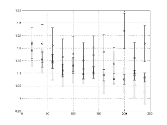
For each value of $n$, we perform a Student’s $t$-test with the null hypothesis being that the average completion time divided by the graph diameter is greater than $1.5$ – against the alternate hypothesis that the same ratio is less than or equal to that (at the $95\%$ confidence level). (Note that the diameter is $(n-1)$.) The results for $n\in\{200,220,240\}$ are shown in Table I. The tests show that we can reject the null hypothesis. In Figure 3 we show the linear dependence of the completion time with respect to the number of agents (and therefore with respect to the diameter) and provide the corresponding $95\%$ confidence intervals.

number of constraints	average completion time/diam	standard deviation	df	$t$-value	$p$-value
$240$	$1.21$	$0.36$	$99$	$-7.73$	$4.3\times 10^{-12}$
$220$	$1.16$	$0.31$	$99$	$-10.90$	$6.0\times 10^{-19}$
$200$	$1.27$	$0.36$	$99$	$-6.49$	$1.7\times 10^{-9}$

TABLE I: Student’s t-test results for demonstrating the linear dependence of the completion time with respect to the diameter. Problem: Graph = line graph, LP model = Model A, $d=4$, $n\in\{200,220,240\}$, ${N}_{\textup{run}}=100$, null hypothesis: average completion time $/n>1.5$.

Figure 3: Average completion time for increasing number of constraints $n$. Specifically: Graph = line graph, LP model = Model A, $d=4$, $n\in\{20,\dots,240\}$, ${N}_{\textup{run}}=100$, performance = average. The solid line is the least-square interpolation of the average completion times.

Next, we aim to upper bound the worst-case completion time. To do so we use a Monte Carlo probability estimation method, that we review from [40].

Remark V.1 (Probability estimation via Monte Carlo)

We aim to estimate the probability that a random variable is less than or equal to a given threshold. Let $Q$ be a compact set and $\Delta$ be a random variable taking values in $Q$. Given a scalar threshold $\gamma$, define the probability $p(\gamma)=\text{Pr}\{J(\Delta)\leq\gamma\}$, where $J:Q\rightarrow{\mathbb{R}}$ is a given measurable performance function. We estimate $p(\gamma)$ as follows. First, we generate $N\in{\mathbb{Z}_{>0}}$ independent identically distributed random samples $\Delta^{(1)},\ldots,\Delta^{(N)}$. Second, we define the indicator function $\mathbb{I}_{J,\gamma}:Q\rightarrow\{0,1\}$ by $\mathbb{I}_{J,\gamma}(\Delta)=1$ if $J(\Delta)\leq\gamma$, and $0$ otherwise. Third and final, we compute the empirical probability as

$$\hat{p}_{N}(\gamma)=\frac{1}{N}\sum_{i=1}^{N}\mathbb{I}_{J,\gamma}(\Delta^{(i)}).$$

Next, we adopt the Chernoff bound in order to provide a bound on the number of random samples required for a certain level of accuracy on the probability estimate. For any accuracy $\epsilon\in(0,1)$ and confidence level $1-\eta\in(0,1)$, we know that $\|\hat{p}_{N}(\gamma)-p(\gamma)\|<\epsilon$ with probability greater than $1-\eta$ if

$$N\geq\frac{1}{2\epsilon^{2}}\log\frac{2}{\eta}.$$ (8)

For $\epsilon=\eta=0.01$, the Chernoff bound (8) is satisfied by $N=27000$ samples. $\square$

Adopting the same notation as in Remark V.1, here is our setup: First, the random variable of interest is a collection of $n$ unit-length vectors (i.e., our random variable takes values in the compact space $\{x\in{\mathbb{R}}^{4}\;|\;\|x\|=1\}^{n}$). Second, the function $J$ is the completion time of the constraints consensus algorithm in solving a nominal problem with constraints determined by $\Delta$. Third, we want to estimate the probability that, for $n\in\{40,60,80\}$, the completion time is less than or equal to $4$ times the diameter of the chain graph of dimension $n$. In order to achieve an accuracy $0.01$ with confidence level $99\%$, we run ${N}_{\textup{run}}=27000$ experiments for each value of $n$ and we compute the maximum completion time in each case. The experiments show that for each $n$ the worst-case completion time is less than $3.4$ times the graph diameter. Therefore, we have established the following statement.

With $99\%$ confidence level, there is at least $99\%$ probability that a nominal problem ($d=4$, graph = line graph, LP model = Model A) with number of constraints $n\in\{40,60,80\}$ is solved by the constraints consensus algorithm in time upper bounded by $4(n-1)$.

V-E Time complexity results for variations of the nominal problems

Next we perform a comparison among different graph models, LP models and LP dimensions. In order to compare the performance of different graphs we consider problems with: Graph $\in$ {line graph, Erdős-Rènyi graph, random geometric graph}, LP model = Model A, $d=4$, $n\in\{20,\dots,240\}$, ${N}_{\textup{run}}=100$. We compute the average completion time to diameter ratio for increasing values of $n$. The results with the $95\%$ confidence interval are shown in Figure 4.

Figure 4: Comparing completion time to diameter ratio for distinct graphs and for increasing number of constraints $n$. Specifically: Graph $\in$ {line graph (circle), Erdős-Rènyi graph (square), random geometric graph (diamond)}, LP model = Model A, $d=4$, $n\in\{20,\dots,240\}$, ${N}_{\textup{run}}=100$, performance = average.

.

To compare the performance for different LP models, we consider problems with: Graph = line graph, LP model $\in$ {Model A, Model B}, $d=4$, $n\in\{20,\dots,240\}$, ${N}_{\textup{run}}=100$. The results with the $95\%$ confidence interval are shown in Figure 5.

Figure 5: Comparing completion time to diameter ratio for distinct LP models and for increasing number of constraints $n$. Specifically: Graph = line graph, LP model $\in$ {Model A (circle), Model B (diamond)} $d=4$, $n\in\{20,\dots,240\}$, ${N}_{\textup{run}}=100$, performance = average.

.

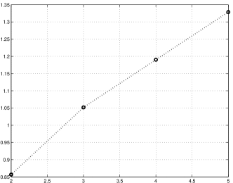
Next, to compare the performance for different dimensions $d$, we consider problems with: Graph = line graph, LP model = Model A, $d\in\{2,3,4,5\}$, $n\in\{20,\dots,240\}$, ${N}_{\textup{run}}=100$. The results with the $95\%$ confidence interval are shown in Figure 6. The comparisons show that, the linear dependence of the completion time with respect to the number of constraints is not affected by the graph topology, the LP model and the dimension $d$. As regards the dimension $d$, as expected, for fixed $n$ the average completion time grows with the dimension. Also, the growth appears to be linear for $d\geq 3$ (for $d=2$ the algorithm seems to perform much better). In Figure 7 we plot the least square value of the completion time to diameter ratio over the number of agents $n$ versus the dimension $d$.

Figure 6: Comparing completion time to diameter ratio for distinct problem dimensions $d$ and for increasing number of constraints $n$. Specifically: Graph = line graph, LP model = Model A, $d\in\{2(square),3(diamond),4(circle),5(triangle)\}$, $n\in\{20,\dots,240\}$, ${N}_{\textup{run}}=100$, performance = average.

.

Figure 7: Comparing completion time to diameter ratio (least square value in $n$) for increasing problem dimensions $d$. Specifically: Graph = line graph, LP model = Model A, $d\in\{2,3,4,5\}$, $n\in\{20,\dots,240\}$, ${N}_{\textup{run}}=100$, performance = average.

.

VI Application to target localization in sensor networks

In this section we discuss an application of distributed abstract programming to sensor networks, namely a distributed solution for target localization. Essentially, we propose a distributed algorithm to approximately compute the intersection of time-varying convex polytopes.

VI-A Motion and sensing models

We consider a target moving on the plane with unknown but bounded velocity. The first-order dynamics is given by

$$p(t+1)=p(t)+v(t),$$ (9)

where $p(t)\in{[{x}_{\textup{min}},{x}_{\textup{max}}]\times[{y}_{\textup{min}},{y}_{\textup{max}}]}\subset{\mathbb{R}}^{2}$ is the target position at time $t\in{\mathbb{Z}_{\geq 0}}$ and $v(t)\in{\mathbb{R}}^{2}$ is unknown but satisfies $\|v\|{}\leq{v}_{\textup{max}}$ for given ${v}_{\textup{max}}$.

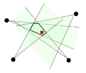
A set of sensors $\{1,\dots,n\}$ deployed in the environment measures the target position. We assume that the measurement noise is unknown and such that, at each time instant, each sensor $i$ measures a possibly-unbounded region of the plane, ${h}^{[i]}(p(t))\subset{\mathbb{R}}^{2}$, containing the target. The set $M(p(t))={\operatorname{\cap}}_{i\in\{1,\dots,n\}}{h}^{[i]}(p(t))$, called the measurement set, provides the best estimate of the target position based on instantaneous measures only. An example scenario is illustrated in Figure 8. In what follows, we make a critical assumption and a convenient one. First, we assume that each measured region ${h}^{[i]}(p(t))$ is a possibly-unbounded convex polygon. Second, for simplicity of notation, we assume that each measured region ${h}^{[i]}(p(t))$ is a half-plane, so that the measurement set $M(p(t))$ is a non-empty possibly-unbounded convex polygon equal with up to $n$ edges.

Figure 8: The measurement set is the intersection of the $4$ sensor measurements.

VI-B Set-membership localization of a moving target

Problem VI.1 (Set-membership localization)

Compute the smallest set $E(t)\subset{\mathbb{R}}^{2}$ that contains the target position $p(t)$ at $t\in{\mathbb{Z}_{\geq 0}}$ and that is consistent with the dynamic model (9) and the sensor measurements ${h}^{[i]}(p(t))$, $i\in\{1,\dots,n\}$. $\square$

We adopt the set-membership approach described in [25]. For $t\in{\mathbb{Z}_{>0}}$, define the sets $E(t|t-1)$ and $E(t|t)$ as the feasible position sets containing all the target positions at time $t$ that are compatible with the dynamics and the available measurements up to time $t-1$ and $t$, respectively. With this notation, the recursion equations are:

$$E(0|0) =M(p(0)),$$ (10a)

$$E(t|t-1) =E(t-1|t-1)+B(0,{v}_{\textup{max}}),$$ (10b)

$$E(t|t) =E(t|t-1)\operatorname{\cap}M(p(t)),$$ (10c)

where the sum set of two sets $A+B$ is defined as $\{a+b\;|\;a\in A\text{ and }b\in B\}$. Equation (10b) is justified as follows: since the target speed satisfies $\|v\|{}\leq{v}_{\textup{max}}$, if the target is at position $p$ at time $t$, then the target must be inside $B(p,{v}_{\textup{max}}\tau)$ at time $t+\tau$, for any positive $\tau$. Equation (10c) is a direct consequence of the definition of measurement set. Equations (10a),  (10b), and (10c) are referred to as initialization, time update and measurement update, respectively. The time and measurement updates are akin to prediction and correction steps in Kalman filtering.

Figure 9: Set-membership localization recursion (10): initialization, time update and measurement update.

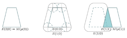
Running the recursion (10) in its exact form is often computationally intractable due to the large and increasing amount of data required to describe the sets $E(t|t-1)$ and $E(t|t)$. To reduce the computational complexity one typically over-approximates these sets with bounded-complexity simple-structure sets, called approximating sets. For example, a common approximating set is the axis-aligned bounding box, i.e., the smallest rectangle aligned with the reference axes containing the set. If $\Pi$ denotes the projection from the subsets of ${\mathbb{R}}^{2}$ onto the collection of approximating sets, then the recursion (10) is rewritten as

$$E(0|0) =\Pi(M(p(0))),$$ (11a)

$$E(t|t-1) =\Pi(E(t-1|t-1)+B(0,{v}_{\textup{max}})),$$ (11b)

$$E(t|t) =\Pi(E(t|t-1)\operatorname{\cap}M(p(t))),$$ (11c)

where now the sets $E(t|t-1)$ and $E(t|t)$ are only approximations of the feasible position sets.

VI-C A centralized LP-based implementation: the eight half-planes algorithm

In this section we propose a convenient choice of approximating sets for set-membership localization and we discuss the corresponding time and measurement updates. We begin with some preliminary notation.

We let $\mathcal{H}_{k}$ be the set containing all possible collections of $k$ half-planes; in other words, an element of $\mathcal{H}_{k}$ is a collection of $k$ half-planes. Given an angle $\theta\in{[0,2\pi[}$ and a set of half-planes $H=\{h_{1},\ldots,h_{k}\}\in\mathcal{H}_{k}$ with $h_{i}=\{x\in{\mathbb{R}}^{2}\;|\;a_{i}^{T}x\leq b_{i},\|a_{i}\|{}=1,b_{i}\in{\mathbb{R}}\}$, define the linear program $(H,\theta)$ by

$$\begin{split}\max&\quad[\cos(\theta)\;\;\sin(\theta)]\cdot x\\ \text{subject to}&\quad a_{i}^{T}x\leq b_{i},\quad i\in\{1,\dots,k\},\\ &\quad{x}_{\textup{min}}\leq{x}\leq{x}_{\textup{max}},\quad{y}_{\textup{min}}\leq{y}\leq{y}_{\textup{max}}.\end{split}$$ (12)

As in Example II.1, transcribe $(H,\theta)$ into an abstract optimization program $(H,\phi_{\theta})$. Recall that $(H,\phi_{\theta})$ is basis regular and has combinatorial dimension $2$, so that its solution, i.e., the lexicographically-minimal minimum point of $(H,\theta)$, is always a set of $2$ constraints, say ${h}^{[1]}_{H,\theta}$ and ${h}^{[2]}_{H,\theta}$. In other words, the pair $\{{h}^{[1]}_{H,\theta},{h}^{[2]}_{H,\theta}\}\in\mathcal{H}_{2}$ is computed as a function of an angle $\theta\in{[0,2\pi[}$ and of a $k$-tuple $H=\{h_{1},\ldots,h_{k}\}\in\mathcal{H}_{k}$.

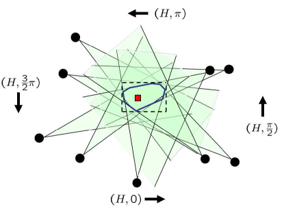
Now, as collection of approximating sets we consider the set $\mathcal{H}_{8}$ containing the collections of $8$ half-planes. Note that the subset of elements $\{h_{1},\dots,h_{8}\}\in\mathcal{H}_{8}$ such that $\operatorname{\cap}_{j=1}^{8}h_{j}$ is bounded is in bijection with the set of convex polygons with at most $8$ edges. Additionally, for arbitrary $k$, we define the projection map $\Pi_{\textup{LP}}:\mathcal{H}_{k}\rightarrow\mathcal{H}_{8}$ as follows: given $H\in\mathcal{H}_{k}$, define $\Pi_{\textup{LP}}(H)\in\mathcal{H}_{8}$ to be the collection of half-planes ${h}^{[1]}_{H,\theta}$ and ${h}^{[2]}_{H,\theta}$, for $\theta\in\{0,\pi/2,\pi,3\pi/2\}$. Note that our approximating set $\Pi_{\textup{LP}}(H)$ contains $H$ and is contained in the smallest axis-aligned bounding box containing $H$; additionally, note that $\Pi_{\textup{LP}}(H)$ contains some possibly repeated half-planes because the same half-plane could be part of the solution for distinct values of $\theta$.

Our definition of $\Pi_{\textup{LP}}$ has the following interpretation: assuming the target is known to satisfy all half-plane constraints in a set $H$, the reduced-complexity possibly-unbounded polygon containing the target is computed by solving four linear programs $(H,\theta)$, $\theta\in\{0,\pi/2,\pi,3\pi/2\}$; see Figure 10.

Figure 10: The eight constraint half-planes (solid thick lines) are determined by the projection $\Pi_{\textup{LP}}$. The dashed rectangle is the smallest axis-aligned bounding box containing the measurement set.

Finally, we review the approximated set-membership localization recursion (11). We assume ${h}^{[i]}(t)=\{x\in{\mathbb{R}}^{2}\;|\;{a}^{[i]}(t)^{T}x\leq{b}^{[i]}(t),\|a_{i}\|{}=1\}$ is the half-plane containing the target measured by sensor $i\in\{1,\dots,n\}$ at time $t\in{\mathbb{Z}_{\geq 0}}$. The approximated feasible position sets, elements of $\mathcal{H}_{8}$, are

$${E}(t|t-1) =\{{h}_{1}(t|t-1),\dots,{h}_{8}(t|t-1)\},\enspace\text{and}$$

$${E}(t|t) =\{{h}_{1}(t|t),\dots,{h}_{8}(t|t)\}.$$

Initialization: Equation (11a) reads

$$\{h_{1}(0|0),\dots,h_{8}(0|0)\}=\Pi_{\textup{LP}}\big{(}\{{h}^{[1]}(0),\dots,{h}^{[n]}(0)\}\big{)}.$$

Time update: Assume $h_{i}(t|t)=\{x\in{\mathbb{R}}^{2}\;|\;{a}_{i}(t)^{T}x\leq{b}_{i}(t)\}$, that is, $h_{i}(t|t)$ is characterized by the coefficients $({a}_{i}(t),{b}_{i}(t))$. Since the target speed satisfies $\|v\|{}\leq{v}_{\textup{max}}$, at instant $t+\tau$ the target is contained in the half-planes

$$h_{i}(t+\tau|t)=\{x\in{\mathbb{R}}^{2}\;|\;{a}_{i}(t)^{T}x\leq{b}_{i}(t)+{v}_{\textup{max}}\tau\}.$$

Therefore, the time update consists in defining each $h_{i}(t+1|t)$ to be $({a}_{i}(t),{b}_{i}(t)+{v}_{\textup{max}})$; we refer to this operation as to a time-translation by an amount ${v}_{\textup{max}}$ of the half-plane $h_{i}(t|t)$. This time-update operation is equivalent to equation (11b) and does not explicitly require an application of the projection $\Pi_{\textup{LP}}$.

Measurement update: Equation (11c) reads

$$\{h_{1}(t|t),\dots,h_{8}(t|t)\}=\Pi_{\textup{LP}}(H(t)),$$

where the collection of constraints at time $t$ is

$$H(t)=\{h_{1}(t|t-1),\dots,h_{8}(t|t-1)\}\cup\{{h}^{[1]}(t),\dots,{h}^{[n]}(t)\}.$$

Remark VI.2

1. During each iteration of the localization recursion, the time update step requires $8$ sums and the measurement update steps requires the solution of $4$ linear programs in $2$ variables and $n+8$ constraints.

2. Similar localization algorithms arise by selecting $\ell\geq 3$ and by solving $\ell$ LP at each iteration parametrized by $\theta\in\{0,2\pi/\ell,\dots,2(\ell-1)\pi/\ell\}$. Larger values of $\ell$ lead to tighter approximating polygons. $\square$

VI-D A distributed eight half-planes algorithm

We consider a scenario in which the sensors measuring the target position also have computation and communication capabilities so that they form a synchronous network as described in Section III. Let ${\mathcal{G}}_{\textup{sn}}=(\{1,\dots,n\},{E}_{\textup{sn}})$ be the undirected communication graph among the sensors $\{1,\dots,n\}$; assume $\mathcal{G}$ is connected. Assume the sensors communicate at each time $t\in{\mathbb{Z}_{\geq 0}}$ and perform measurements of the target at unspecified times in ${\mathbb{Z}_{\geq 0}}$ (communication takes place at higher rate than sensing). For simplicity, we assume the first measurement at each node happens at time $0$.

We aim to design a distributed algorithm for the sensor network to localize a moving target. The idea is to run local set-membership recursions (with time and measurement updates) at each node while exchanging constraints in order to achieve constraints consensus on a set-membership estimate. Distributed constraint re-examination is obtained as follows: at each time, each node keeps in memory the last $m$ measurements it took and, after an appropriate time-update, re-introduces them into the $\Pi_{\textup{LP}}$ computation. We begin with an informal description.

Eight Half-Planes Consensus Algorithm: The processor state at each processor $i$ contains a set $H^{[i]}_{\textup{optimal}}$ of $8$ candidate optimal constraints and a set $H^{[i]}_{\textup{sensed}}$ containing the last $m$ measurements, for some $m>0$. These sets are initialized to the first sensor measurement. At each communication round, the processor performs the following tasks: (i) it transmits $H^{[i]}_{\textup{optimal}}$ to its out-neighbors and acquires from its in-neighbors their candidate constraints; (ii) it performs a time-update, that is, a time-translation by an amount ${v}_{\textup{max}}$, of all candidate optimal, measured and received constraints; (iii) it updates the set of measured constraints if a new measurement is taken; and (iv) it updates $H^{[i]}_{\textup{optimal}}$ to be the projection $\Pi_{\textup{LP}}$ of all candidate optimal, measured and received constraints.

Next we give a pseudo-code description.

 

Problem data:

A network ${\mathcal{G}}_{\textup{sn}}$ of sensors that measure half-plane constraints

Algorithm:

Eight Half-Planes Consensus

Message alphabet:

$\mathbb{A}=\mathcal{H}_{8}\cup\{\textup{{null}}\}$

Processor state:

$H^{[i]}_{\textup{optimal}}\in\mathcal{H}_{8}$

$H^{[i]}_{\textup{sensed}}\in\mathcal{H}_{m}$ for some $m>0$

Initialization:

$H^{[i]}_{\textup{optimal}}:=\{{h}^{[i]}(0),\dots,{h}^{[i]}(0)\}$

$H^{[i]}_{\textup{sensed}}:=\{{h}^{[i]}(0),\dots,{h}^{[i]}(0)\}$

function $\textup{msg}\big{(}(H^{[i]}_{\textup{optimal}},H^{[i]}_{\textup{sensed}}),j\big{)}$

1:  return $H^{[i]}_{\textup{optimal}}$

function $\textup{stf}\big{(}(H^{[i]}_{\textup{optimal}},H^{[i]}_{\textup{sensed}}),y\big{)}$
% executed by node $i$, with $y_{j}:=H^{[j]}_{\textup{optimal}}$

1:  time-translate by an amount ${v}_{\textup{max}}$ all constraints constraints in $H^{[i]}_{\textup{sensed}}$, $H^{[i]}_{\textup{optimal}}$, and $\cup_{j\in{\mathcal{N}}_{\textup{in}}(i)}y_{j}$

2:  if a new measurement is taken at this time, then

3:     add it to $H^{[i]}_{\textup{sensed}}$; drop oldest measurement from $H^{[i]}_{\textup{sensed}}$

4:  end if

5:  set $H^{[i]}_{\textup{optimal}}:=\Pi_{\textup{LP}}\Big{(}H^{[i]}_{\textup{sensed}}\cup H^{[i]}_{\textup{optimal}}\cup_{j\in{\mathcal{N}}_{\textup{in}}(i)}y_{j}\Big{)}$

6:  return $(H^{[i]}_{\textup{optimal}},H^{[i]}_{\textup{sensed}})$

 

Finally, we collect some straightforward facts about this algorithm; we omit the proof in the interest of brevity.

Proposition VI.3

(Properties of the eight half-planes consensus algorithm) Consider a connected network ${\mathcal{G}}_{\textup{sn}}$ of sensors that measure half-plane constraints and that implement the eight half-plane consensus algorithm. Assume the target does not move, that is, set ${v}_{\textup{max}}=0$. The following statements hold:

1. the candidate optimal constraints at each node contain the target at each instant of time;

2. the candidate optimal constraints at each node monotonically improve over time; and

3. additionally, if each node makes at most $m$ measurements in finite time, then the candidate optimal constraints at each node converge in finite time to the globally optimal $8$ half-plane constraints.

Next, let us state some memory complexity bounds for the eight half-plane consensus algorithm. Again, we adopt the convention that a memory unit is the amount of memory required to store a constraint in $H$. Each node $i$ of the network requires $(8+m+8\operatorname{card}({\mathcal{N}}_{\textup{in}}(i)))$ memory units in order to implement the algorithm. If we assume that number $m$ of stored measurements is independent of $n$ and that the indegree of each node is bounded irrespectively of $n$, then the algorithm memory complexity is in $O(1)$. Vice-versa, in worst-case graphs, the algorithm memory complexity is in $O(n)$.

VII Application to formation control for robotic networks

In this section we apply constraints consensus ideas to formation control problems for networks of mobile robots. We focus on formations with the shapes of a point, a line, or a circle. (The problem of formation control to a point is usually referred to as the rendezvous or gathering problem.) We solve these formation control problems in a time-efficient manner via a distributed algorithm regulating the communication among robots and the motion of each robot.

VII-A Model of robotic network

We define a robotic network as follows. Each robot is equipped with a processor and robots exchange information via a communication graph. Therefore, the group of robots has the features of a synchronous network and can implement distributed algorithms as defined in Section III. However, as compared with a synchronous network, a robotic network has two distinctions: (i) robots control their motion in space, and (ii) the communication graph among the robots depends upon the robots positions, rather than time.

Specifically, the robotic network evolves according to the following discrete-time communication, computation and motion model. Each robot $i\in\{1,\dots,n\}$ moves between rounds according to the first order discrete-time integrator ${p}^{[i]}(t+1)={p}^{[i]}(t)+{u}^{[i]}(t)$, where ${p}^{[i]}\in{\mathbb{R}}^{2}$ and $\|{u}^{[i]}\|^{2}\leq{u}_{\textup{max}}>0$. At each discrete time instant, robots at positions $P_{n}$ communicate according to the disk graph ${\mathcal{G}}_{\textup{disk}}(P_{n})=(\{1,\dots,n\},{E}_{\textup{disk}}(P_{n}))$ defined as follows: an edge $(i,j)\in\{1,\dots,n\}^{2}$, $i\neq{j}$, belongs to ${E}_{\textup{disk}}(P_{n})$ if and only if $\|{p}^{[i]}-{p}^{[j]}\|{}\leq{r}_{\textup{cmm}}$ for some ${r}_{\textup{cmm}}>0$.

A distributed algorithm for a robotic network consists of (1) a distributed algorithm for a synchronous network, that is, a processor state, a message alphabet, a message-generation and a state-transition function, as described in Section III, (2) an additional function, called the control function, that determines the robot motion, with the following domain and co-domain:

$$\textup{ctl}:{\mathbb{R}}^{2}\times W\times\mathbb{A}^{n}\rightarrow B(0,{u}_{\textup{max}}).$$

Additionally, we here allow the message generation and the state transition to depend upon not only the processor state but also the robot position. The state of the robotic network evolves as follows. First, at each communication round $t$, each processor $i$ sends to its outgoing neighbors a message computed by applying the message-generation function to the current values of ${p}^{[i]}$ and ${w}^{[i]}$. After a negligible period of time, the $i$th processor resets the value of its processor state ${w}^{[i]}$ by applying the state-transition function to the current values of ${p}^{[i]}$ and ${w}^{[i]}$, and to the messages received at time $t$. Finally, the position ${p}^{[i]}$ of the $i$th robot at time $t$ is determined by applying the control function to the current value of ${p}^{[i]}$ and ${w}^{[i]}$, and to the messages received at time $t$.

In formal terms, if ${y}^{[i]}(t)$ denotes the message vector received at time $t$ by agent $i$ (with ${y}^{[i]}_{j}(t)$ being the message received from agent $j$), then the evolution is determined by

$$\begin{split}{y}^{[i]}_{j}(t)&=\textup{msg}(p^{[j]}(t-1),w^{[j]}(t-1),i),\\ {w}^{[i]}(t)&=\textup{stf}(p^{[i]}(t-1),{w}^{[i]}(t-1),y^{[i]}(t)),\\ p^{[i]}(t)&=p^{[i]}(t-1)+\textup{ctl}(p^{[i]}(t-1),{w}^{[i]}(t),y^{[i]}(t)),\end{split}$$

with the convention that $\textup{msg}(p^{[j]}(t-1),w^{[j]}(t-1),i)=\textup{{null}}$ if $(i,j)\not\in{E}_{\textup{disk}}(p^{[1]}(t-1),\dots,p^{[n]}(t-1))$.

VII-B Formation tasks and related optimization problems

Numerous definitions of robot formation are considered in the multi-agent literature. Here we consider a somehow specific situation. Let ${S}_{\textup{points}}$, ${S}_{\textup{lines}}$, and ${S}_{\textup{circles}}$ be the set of points, lines and circles in the plane, respectively. We refer to these three sets as the shape sets. We aim to lead all robots in a network to a single element of one of the shape sets If $S$ is a selected shape set, the formation task is achieved by the robotic network if there exists a time $T\in{\mathbb{Z}_{>0}}$ such that for all $t\geq T$, all robots $i\in\{1,\dots,n\}$ satisfy ${p}^{[i]}(t)\in s$ for some element $s\in S$. Specifically, the point-formation, or rendezvous task requires all connected robots to be at the same position, the line-formation task requires all connected robots to be on the same line, and the circle-formation task requires all connected robots to be on the same circle.

We are interested in distributed algorithms that achieve such formation tasks optimally with respect to a suitable cost function. For the point-formation and line-formation tasks, we aim to minimize completion time, i.e., the time required by all robots to reach a common shape. For the circle-formation task, we aim to minimize the product between the time required to reach a common circle, and the diameter of the common circle.

Remark VII.1 (Circle formation)

For the circle-formation problem we do not select the completion time as cost function, because of the following reasons. The centralized version of the minimum time circle-formation problem is equivalent to finding the minimum-width annulus containing the point-set. For arbitrary data sets, the minimum-width annulus has arbitrarily large minimum radius and bears similarities with the solution to the smallest stripe problem. For some configurations, all points are contained only in a small fraction of the minimum-width annulus; this is not the solution we envision when we consider moving robots in a circle formation. Therefore, we consider, instead, the smallest-area annulus. This cost function penalizes both the difference of the radiuses of the annulus (width of the annulus) and their sum. $\square$

The key property of the minimum-time point-formation task, minimum-time line-formation task, and optimum circle-formation task is that their centralized versions are equivalent to finding the smallest ball, stripe and annulus, respectively, enclosing the $n$ agents’ initial positions. We state these equivalences in the following lemma without proof.

Lemma VII.2 (Optimal shapes from geometric optimization)

Given a set of distinct points $\{p_{1},\dots,p_{n}\}\subset{\mathbb{R}}^{2}$, consider the three optimization problems:

$$\begin{split}\min_{p\in{S}_{\textup{points}}}\;\max_{j\in\{1,\dots,n\}}&\;\|p_{j}-p\|{},\\ \min_{\ell\in{S}_{\textup{lines}}}\;\max_{j\in\{1,\dots,n\}}&\;\operatorname{dist}(p_{j},\ell),\\ \min_{c\in{S}_{\textup{circles}}}\;\max_{j\in\{1,\dots,n\}}&\;\operatorname{dist}(p_{j},c)\cdot\operatorname{radius}(c),\end{split}$$

where $\operatorname{radius}(c)$ denotes the radius of the circle $c$. These three optimization problems are equivalent to the smallest enclosing ball, the smallest enclosing stripe (for points in stripe-generic position), and the smallest enclosing annulus problem, respectively.

Therefore, they are abstract optimization problems with combinatorial dimension $3$, $5$ and $4$, respectively.

We conclude this section with some useful notation. We let $\texttt{target\_set}(\{p_{1},\dots,p_{n}\})$ denote the point, the line or the circle equidistant from the boundary of the smallest enclosing ball, stripe or annulus, respectively.

VII-C Connectivity assumption, objective and strategy

We assume that the robotic network is connected at initial time, i.e., that the graph ${\mathcal{G}}_{\textup{disk}}(P_{n}(0))$ is connected, and we aim to achieve the formation task while guaranteeing that the state-dependent communication graph remains connected during the evolution. The following connectivity maintenance strategy was originally proposed in [28] and a comprehensive discussion is in [41]. The key idea is to restrict the allowable motion of each robot so as to preserve the existing edges in the communication graph. We present this idea in three steps.

First, in a network with communication edges ${E}_{\textup{disk}}$, if agents $i$ and $j$ are neighbors at time $t\in{\mathbb{Z}_{\geq 0}}$, then we require that their positions at time $t+1$ belong to

$$\mathcal{X}({p}^{[i]}(t),{p}^{[j]}(t))=B\Big{(}\frac{{p}^{[i]}(t)+{p}^{[j]}(t)}{2},\frac{1}{2}{r}_{\textup{cmm}}\Big{)}.$$

If all neighbors of agent $i$ at time $t$ are at locations ${Q}^{[i]}(t)=\{q_{1},\dots,q_{l}\}$, then the (convex) constraint set of agent $i$ is

$$\mathcal{X}({p}^{[i]}(t),{Q}^{[i]}(t))=\bigcap_{q\in\{q_{1},\dots,q_{l}\}}B\Big{(}\frac{{p}^{[i]}(t)+q}{2},\frac{1}{2}{r}_{\textup{cmm}}\Big{)}.$$

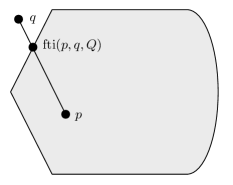
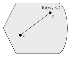
Second, given $p$ and $q$ in ${\mathbb{R}}^{2}$ and a convex closed set $Q\subset{\mathbb{R}}^{2}$ with $p\in Q$, we introduce the from-to-inside function, denoted by fti and illustrated in Figure 11, that computes the point in the closed segment $[p,q]$ which is at the same time closest to $q$ and inside $Q$. Formally,

$$\text{fti}(p,q,Q)=\begin{cases}q,&\text{if }q\in Q,\\ [p,q]\operatorname{\cap}\partial Q,\quad&\text{if }q\notin Q.\end{cases}$$

Figure 11: Illustration of the fti function; courtesy of the authors of [41].

Third and final, we assume that, independent of whatever control algorithm dictates the robots evolution, if ${p}^{[i]}_{\text{target}}(t)$ denote the desired target positions of agent $i$ at time $t+1$, then we allow robot $i$ to move towards that location only so far as the constraint set allows. This is encoded by:

$${p}^{[i]}(t+1)=\text{fti}({p}^{[i]}(t),{p}^{[i]}_{\text{target}}(t),\mathcal{X}({p}^{[i]}(t),{Q}^{[i]}(t))).$$

VII-D Move-to-consensus-shape strategy

The minimum-time point-formation, minimum-time line-formation, and optimum circle formation tasks appear intractable in their general form due to the state-dependent communication constraints. To attack these problem, we search for an efficient strategy that converges to the optimal one when the upper bound on the robot speed ${u}_{\textup{max}}$ goes to zero or, in other words, when information transmission tends to be infinitely faster than motion. To design such a strategy, we aim to reach consensus on the centralized solution to the problem, i.e., the optimal shape, and use the solution as a reference for the agents motion.

A simple sequential solution is as follows: first, the agents compute the optimal shape via constraints consensus, and then, when consensus is achieved, they move toward the closest point in the target shape (point, line or circle). An improved strategy allows concurrent execution of constraints consensus and motion: while the constraints consensus algorithm is running, each agent moves toward the estimated target position while maintaining connectivity of the communication graph. We first provide an informal description.

Move-to-consensus-shape strategy: The processor state at each robot $i$ consists of a set ${B}^{[i]}$ of $\delta$ candidate optimal constraints and a binary variable ${halt}^{[i]}\in\{0,1\}$. The set ${B}^{[i]}$ is initialized to ${p}^{[i]}(0)$ and ${halt}^{[i]}$ is initialized to $0$. At each communication round, the processor performs the following tasks: (i) it transmits ${p}^{[i]}$ and ${B}^{[i]}$ to its neighbors and acquires its neighbors’ candidate constraints and their current position; (ii) it runs an instance of the constraints consensus algorithm for the geometric optimization program of interest (smallest enclosing ball, stripe or annulus); if the constraints consensus halting condition is satisfied, it sets ${halt}^{[i]}$ to $1$; (iii) it computes a robot target position based on the current estimate of the optimal shape; (iv) it moves the robot towards the target position while respect input constraint and, if ${halt}^{[i]}$ is still zero, enforcing connectivity with its current neighbors.

Next we give a pseudo-code description. We let $P_{n}(0)=\{{p}^{[1]}(0),\ldots,{p}^{[n]}(0)\}$.

 

Problem data:

A robotic network and a shape set

Algorithm:

Move-to-Consensus-Shape

Message alphabet:

$\mathbb{A}={\mathbb{R}}^{2}\cup({\mathbb{R}}^{2})^{\delta}\cup\{\textup{{null}}\}$

Processor state:

${B}^{[i]}\subset P_{n}(0)$ with $\operatorname{card}({B}^{[i]})=\delta$

${\texttt{halt}}^{[i]}\in\{0,1\}$

Physical state:

${p}^{[i]}\in{\mathbb{R}}^{2}$

Initialization:

${B}^{[i]}:=\{{p}^{[i]}(0),\dots,{p}^{[i]}(0)\}$

${\texttt{halt}}^{[i]}:=0$

function $\textup{msg}\big{(}{p}^{[i]},{B}^{[i]},j\big{)}$

1:  return $({p}^{[i]},{B}^{[i]})$

function $\textup{stf}\big{(}{B}^{[i]},{\texttt{halt}}^{[i]},y\big{)}$
% executed by node $i$, with $y_{j}=({p}^{[j]},{B}^{[j]}):=\textup{msg}({B}^{[j]},i)$

1:  ${S}_{\textup{tmp}}:=\{{p}^{[i]}(0)\}\cup{B}^{[i]}\cup\big{(}\cup_{j\in{\mathcal{N}}_{\textup{in}}(i)}{B}^{[j]}\big{)}$

2:  ${B}^{[i]}:=\textup{{Subex\_LP}}({S}_{\textup{tmp}},{B}^{[i]})$

3:  if ${B}^{[i]}$ has not changed for $2n$ rounds,

4:   then ${\texttt{halt}}^{[i]}:=1;$  end if

5:  return $({B}^{[i]},{\texttt{halt}}^{[i]})$

function $\textup{ctl}\big{(}{B}^{[i]},{p}^{[i]},y\big{)}$
% executed by node $i$, with $y_{j}=({p}^{[j]},{B}^{[j]}):=\textup{msg}({B}^{[j]},i)$
% map target_set defined in Section VII-B

1:  ${S}_{\textup{{trgt}}}:=\texttt{target\_set}({B}^{[i]})$

2:  $\displaystyle{p}_{\textup{trgt}}:=\arg\min_{p\in{S}_{\textup{{trgt}}}}\|{p}^{[i]}-p\|{}$

3:  if ${\texttt{halt}}^{[i]}=0$, then${\mathcal{X}}_{\textup{cnstr}}:=\bigcap_{j\in{\mathcal{N}}_{\textup{in}}(i)}B\Big{(}\frac{{p}^{[i]}+{p}^{[j]}}{2},\frac{1}{2}{r}_{\textup{cmm}}\Big{)}\bigcap B\big{(}{p}^{[i]},{u}_{\textup{max}}\big{)}$else ${\mathcal{X}}_{\textup{cnstr}}:=B\big{(}{p}^{[i]},{u}_{\textup{max}}\big{)};$  end if

4:  return $\text{fti}({p}^{[i]},{p}_{\textup{trgt}},{\mathcal{X}}_{\textup{cnstr}})-{p}^{[i]}$

 

We refer the interested reader to [1] for numerical simulation results for the move-to-consensus-shape strategy. Finally, we state the correctness of the algorithm and omit the proof in the interest of brevity.

Proposition VII.3

(Properties of the move-to-consensus-shape algorithm) On a robotic network with communication graph ${G}_{\textup{disk}}$ and bounded control inputs ${u}_{\textup{max}}$, the move-to-consensus-shape strategy achieves the desired formation control tasks.

In the limit as ${u}_{\textup{max}}\to 0^{+}$, the move-to-consensus-shape strategy solves the optimal formation control tasks, i.e., the minimum-time point-formation, minimum-time line-formation, and optimum circle formation tasks.

VIII Conclusions

We have introduced a novel class of distributed optimization problems and proposed a simple and intuitive algorithmic approach. Additionally, we have rigorously established the correctness of the proposed algorithms and presented a thorough Monte Carlo analysis to substantiate our conjecture that, for a broad variety of settings, the time complexity of our algorithms is linear. Finally, we have discussed in detail two modern applications: target localization in sensor networks and formation control in robotic networks.

Promising avenues for further research include proving the linear-time-complexity conjecture, as well as applying our algorithms to (i) optimization problems for randomly switching graphs and gossip communication, (ii) distributed machine learning problems [22, 21, 23], and (iii) convex quadratic programming [42]. Additionally, it is of interest to verify the performance of our proposed target localization and formation control algorithms in experimental setups.

Abstract framework for the smallest enclosing stripe problem

In this appendix we consider the smallest enclosing stripe problem in Example II.2 for stripe-generic points and show that is satisfies the abstract optimization axioms. We begin with some notation. Let $H$ be the set of constraints, i.e., the set of points in the plane for which we aim to compute the smallest enclosing stripe. With a slight abuse of notation, $h\in H$ denotes both a constraint and a point depending on the context. Let $\phi(G)$, $G\subset H$, be the width of the smallest stripe enclosing the points in $G$. A constraint $h$ is violated by the set $G$, i.e., $\phi(G\cup\{h\})>\phi(G)$, if the point $h$ does not belong to the smallest stripe enclosing $G$.

First, note that three points are necessary, but in general not sufficient, to uniquely identify the smallest enclosing stripe of a set $H$ of three or more points. Indeed, the boundary of the smallest stripe enclosing $H$ contains at least three points of $H$, e.g., point $h_{1}$ on one line and points $\{h_{2},h_{3}\}$ on the other line. So, the smallest enclosing stripe identifies the triplet $\{h_{1},h_{2},h_{3}\}$. However, a simple geometric argument shows that the converse is not true, i.e., three points are not sufficient. Three points would be sufficient if the triplet was an ordered set and uniquely identified a stripe. To uniquely identify the smallest enclosing stripe for a set $H$ of five or more points, one needs to add to the triplet $\{h_{1},h_{2},h_{3}\}$ another two points of $H$ that belong to the correctly stripe among the three stripes determined by $\{h_{1},h_{2},h_{3}\}$. In summary, this discussion shows that the combinatorial dimension is $5$.

Second, we prove that the two axioms of abstract optimization are satisfied. As usual, monotonicity is trivially satisfied, thus we need to prove locality. Suppose, by contradiction, that locality does not hold. Therefore there exist $F$, $G$ and $h$, $F\subset G\subset H$ and $h\in H$, with $-\infty<\phi(F)=\phi(G)$ such that $\phi(G\cup\{h\})>\phi(G)$ and $\phi(F\cup\{h\})=\phi(F)$. Let $S_{G}$ and $S_{F}$ be the smallest stripes for $G$ and $F$, so that $({g}_{\textup{1}},{g}_{\textup{2}},{g}_{\textup{3}})$ and $({f}_{\textup{1}},{f}_{\textup{2}},{f}_{\textup{3}})$ are the ordered triplets of points defining $S_{G}$ and $S_{F}$, respectively. Since $h$ is violated by $G$ but not by $F$, this means that $h$ belongs to $S_{F}$ but not to $S_{G}$. Therefore, the stripes $S_{G}$ and $S_{F}$ must be different, i.e., $({g}_{\textup{1}},{g}_{\textup{2}},{g}_{\textup{3}})\neq({f}_{\textup{1}},{f}_{\textup{2}},{f}_{\textup{3}})$. Because the points are in stripe-generic positions, we know that $\operatorname{dist}({g}_{\textup{1}},l({g}_{\textup{2}},{g}_{\textup{3}}))\neq\operatorname{dist}({f}_{\textup{1}},l({f}_{\textup{2}},{f}_{\textup{3}}))$ and, therefore, $\phi(G)>\phi(F)$. This proves the contradiction.

References

- [1] G. Notarstefano and F. Bullo, “Distributed consensus on enclosing shapes and minimum time rendezvous,” in IEEE Conf. on Decision and Control, San Diego, CA, Dec. 2006, pp. 4295–4300.
- [2] ——, “Network abstract linear programming with application to minimum-time formation control,” in IEEE Conf. on Decision and Control, New Orleans, LA, Dec. 2007, pp. 927–932.
- [3] ——, “Network abstract linear programming with application to cooperative target localization,” in Modelling, Estimation and Control of Networked Complex Systems, ser. Understanding Complex Systems, A. Chiuso, L. Fortuna, M. Frasca, L. Schenato, and S. Zampieri, Eds. Springer, 2009, pp. 177–190.
- [4] J. N. Tsitsiklis, D. P. Bertsekas, and M. Athans, “Distributed asynchronous deterministic and stochastic gradient optimization algorithms,” IEEE Transactions on Automatic Control, vol. 31, no. 9, pp. 803–812, 1986.
- [5] N. Motee and A. Jadbabaie, “Distributed multi-parametric quadratic programming,” IEEE Transactions on Automatic Control, vol. 54, no. 10, 2009.
- [6] A. Nedic, A. Ozdaglar, and P. A. Parrilo, “Constrained consensus and optimization in multi-agent networks,” IEEE Transactions on Automatic Control, 2009, to appear.
- [7] B. Johansson, A. Speranzon, M. Johansson, and K. H. Johansson, “On decentralized negotiation of optimal consensus,” Automatica, vol. 44, no. 4, pp. 1175–1179, 2008.
- [8] D. P. Palomar and M. Chiang, “Alternative distributed algorithms for network utility maximization: Framework and applications,” IEEE Transactions on Automatic Control, vol. 52, no. 12, pp. 2254–2269, 2007.
- [9] J. Matousek, M. Sharir, and E. Welzl, “A subexponential bound for linear programming,” Algorithmica, vol. 16, no. 4/5, pp. 498–516, 1996.
- [10] B. Gärtner, “A subexponential algorithm for abstract optimization problems,” SIAM Journal on Computing, vol. 24, no. 5, pp. 1018–1035, 1995.
- [11] M. Goldwasser, “A survey of linear programming in randomized subexponential time,” SIGACT News, vol. 26, no. 2, pp. 96–104, 1995.
- [12] N. Megiddo, “Linear programming in linear time when the dimension is fixed,” Journal of the Association for Computing Machinery, vol. 31, no. 1, pp. 114–127, 1984.
- [13] B. Gärtner and E. Welzl, “Linear programming - randomization and abstract frameworks,” in Symposium on Theoretical Aspects of Computer Science, ser. Lecture Notes in Computer Science, vol. 1046, 1996, pp. 669–687.
- [14] ——, “A simple sampling lemma: Analysis and applications in geometric optimization,” Discrete & Computational Geometry, vol. 25, no. 4, pp. 569–590, 2001.
- [15] P. K. Agarwal and S. Sen, “Randomized algorithms for geometric optimization problems,” in Handbook of Randomization, P. Pardalos, S. Rajasekaran, J. Reif, and J. Rolim, Eds. Kluwer Academic Publishers, 2001.
- [16] P. K. Agarwal and M. Sharir, “Efficient algorithms for geometric optimization,” ACM Computing Surveys, vol. 30, no. 4, pp. 412–458, 1998.
- [17] M. Ajtai and N. Megiddo, “A deterministic -time -processor algorithm for linear programming in fixed dimension,” SIAM Journal on Computing, vol. 25, no. 6, pp. 1171–1195, 1996.
- [18] Y. Bartal, J. W. Byers, and D. Raz, “Fast, distributed approximation algorithms for positive linear programming with applications to flow control,” SIAM Journal on Computing, vol. 33, no. 6, pp. 1261–1279, 2004.
- [19] H. Dutta and H. Kargupta, “Distributed linear programming and resource management for data mining in distributed environments,” in IEEE Int. Conference on Data Mining, Pisa, Italy, Dec. 2008, pp. 543–552.
- [20] Y. Lu and V. Roychowdhury, “Parallel randomized support vector machine,” in Advances in Knowledge Discovery and Data Mining (10th Pacific-Asia Conference, Singapore 2006), ser. Lecture Notes in Artificial Intelligence, W. K. Ng, M. Kitsuregawa, and J. Li, Eds. Springer, 2006, pp. 205–214.
- [21] Y. Lu, V. Roychowdhury, and L. Vandenberghe, “Distributed parallel support vector machines in strongly connected networks,” IEEE Transactions on Neural Networks, vol. 19, no. 7, pp. 1167–1178, 2008.
- [22] J. Balcázar, Y. Dai, J. Tanaka, and O. Watanabe, “Provably fast training algorithms for support vector machines,” Theory of Computing Systems, vol. 42, no. 4, pp. 568–595, 2008.
- [23] K. Flouri, B. Beferull-Lozano, and P. Tsakalides, “Training a SVM-based classifier in distributed sensor networks,” in European Signal Processing Conference, Florence, Italy, Sep. 2006.
- [24] F. Zhao and L. Guibas, Wireless Sensor Networks: An Information Processing Approach. Morgan-Kaufmann, 2004.
- [25] A. Garulli and A. Vicino, “Set membership localization of mobile robots via angle measurements,” IEEE Transactions on Robotics and Automation, vol. 17, no. 4, pp. 450–463, 2001.
- [26] V. Isler and R. Bajcsy, “The sensor selection problem for bounded uncertainty sensing models,” IEEE Transactions on Automation Sciences and Engineering, vol. 3, no. 4, pp. 372–381, 2006.
- [27] I. Suzuki and M. Yamashita, “Distributed anonymous mobile robots: Formation of geometric patterns,” SIAM Journal on Computing, vol. 28, no. 4, pp. 1347–1363, 1999.
- [28] H. Ando, Y. Oasa, I. Suzuki, and M. Yamashita, “Distributed memoryless point convergence algorithm for mobile robots with limited visibility,” IEEE Transactions on Robotics and Automation, vol. 15, no. 5, pp. 818–828, 1999.
- [29] X. Defago and A. Konagaya, “Circle formation for oblivious anonymous mobile robots with no common sense of orientation,” in ACM Int. Workshop on Principles of Mobile Computing, Toulouse, France, Oct. 2002, pp. 97–104.
- [30] M. Egerstedt and X. Hu, “Formation constrained multi-agent control,” IEEE Transactions on Robotics and Automation, vol. 17, no. 6, pp. 947–951, 2001.
- [31] H. G. Tanner, G. J. Pappas, and V. Kumar, “Leader-to-formation stability,” IEEE Transactions on Robotics and Automation, vol. 20, no. 3, pp. 443–455, 2004.
- [32] J. A. Marshall, M. E. Broucke, and B. A. Francis, “Formations of vehicles in cyclic pursuit,” IEEE Transactions on Automatic Control, vol. 49, no. 11, pp. 1963–1974, 2004.
- [33] R. Shamir, “The efficiency of the simplex method: A survey,” Management Science, vol. 33, no. 3, pp. 301–334, 1987.
- [34] N. A. Lynch, Distributed Algorithms. Morgan Kaufmann, 1997.
- [35] J. M. Hendrickx, “Graphs and networks for the analysis of autonomous agent systems,” Ph.D. dissertation, Université Catholique de Louvain, Belgium, Feb. 2008.
- [36] R. Albert and A.-L. Barabási, “Statistical mechanics of complex networks,” Reviews of Modern Physics, vol. 74, no. 1, pp. 47–97, 2002.
- [37] J. R. Dunham, D. G. Kelly, and J. W. Tolle, “Some experimental results concerning the expected number of pivots for solving randomly generated linear programs,” Operations Research and System Analysis Department, University of North Carolina at Chapel Hill, Tech. Rep. 77-16, 1977.
- [38] K. H. Borgwardt, “Untersuchungenzur Asymptotik der mittleren Schrittzahl von Simplexverfahren in der Linearen Optimierung,” Operations Research-Verfahren, vol. 28, pp. 332–345, 1977.
- [39] M. J. Todd, “Probabilistic models for linear programming,” Mathematics of Operations Research, vol. 16, no. 4, pp. 671–693, 1991.
- [40] R. Tempo, G. Calafiore, and F. Dabbene, Randomized Algorithms for Analysis and Control of Uncertain Systems. Springer, 2005.
- [41] F. Bullo, J. Cortés, and S. Martínez, Distributed Control of Robotic Networks, ser. Applied Mathematics Series. Princeton University Press, 2009, available at http://www.coordinationbook.info.
- [42] R. Goldbach, “Some randomized algorithms for convex quadratic programming,” Applied Mathematics & Optimization, vol. 39, no. 1, pp. 121–142, 1999.