Magnetocaloritronic nanomachines

Abstract

We introduce and study a magnetocaloritronic circuit element based on a domain wall that can move under applied voltage, magnetic field and temperature gradient. We draw analogies between the Carnot machines and possible devices employing such circuit element. We further point out the parallels between the operational principles of thermoelectric and magnetocaloritronic cooling and power generation and also introduce a magnetocaloritronic figure of merit. Even though the magnetocaloritronic figure of merit turns out to be very small for transition-metal based magnets, we speculate that larger numbers may be expected in ferromagnetic insulators.

1 Introduction

There have been numerous realizations of Carnot machines since they were first envisaged by Nicolas Léonard Sadi Carnot, in both direct (i.e., engine) and reverse (i.e., refrigerator or heat pump) modes of operation. While the traditional mechanical Carnot machines are based on the alternating adiabatic and isothermal processes controlled by the conjugate pair of variables ($P$,$V$), same thermodynamic principles can be put to work in the realizations of magnetic machines relying on the magnetocaloric effect [1]. These latter machines are operating in the space of the conjugate variables ($H$,$M$). At nanoscale, however, one might need to rely on different principles and thermoelectric cooling and power generation appear to be very promising [2, 3]. In particular, large values of the thermoelectric figure of merit have recently been suggested for molecular junctions [4]. In this paper, we envision an interplay of the magnetocaloric and thermoelectric functionalities.

A growing interest in spin caloritronics that comprises the spin related phenomena with thermoelectric effects has been spurred recently by many promising applications [5, 6, 7]. Thermoelectric spin transfer relates the heat current to magnetization dynamics [8, 9, 10] while opposite effect of heat currents resulting from magnetization dynamics should also occur [10, 11]. The spin-transfer torque [12, 13] in spin valves and domain walls [14, 15, 16] has been well understood for transition-metal based magnets [17, 18, 19] which already led to many applications [20]. The reciprocal effect to the spin-transfer torque results in electromotive forces induced by the magnetization dynamics [21, 22, 23, 24]. All these pave the way for novel devices that can output as well as be controlled by temperature gradients, electric currents, and magnetic fields. These machines can have similar functionalities as Carnot machines and work at nanoscale.

In this paper, we introduce and describe a magnetocaloritronic circuit element utilizing magnetic domain wall motion. Further, we use this element to demonstrate the principle of magnetocaloritronic cooling and power generation. We also draw parallels between the operational principles of thermoelectric and magnetocaloritronic cooling and power generation. This program naturally leads us to the introduction of the magnetocaloritronic figure of merit $TZ_{\mbox{mc}}$ which encodes information about the maximum efficiency of such devices. Our estimates indicate a very small figure of merit for typical transition-metal based magnets; however, we speculate that one can achieve better efficiencies using the ferromagnetic insulators in which the heat transferred by spin waves will better couple to the texture dynamics in the absence of dissipation related to the electron-hole continuum.

2 Magnetocaloritronic circuit element

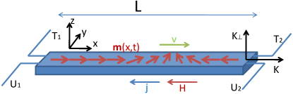
Figure 1: (Color online) A domain-wall based circuit element can be controlled by applying voltage $\Delta U$, magnetic field $H$ and temperature gradient $\Delta T$. Here, we consider transverse head-to-head Néel domain wall parallel to the $y$ axis in the easy $xy$ plane. The constants $K$ and $K_{\perp}$ describe the easy axis and easy plane anisotropy.

In order to explore new functionalities, we introduce a domain-wall based circuit element (see Fig. 1) that combines the capabilities of a thermoelectric contact, heat pump and generator of electromagnetic field. The functionalities of this circuit element can be controlled directly by applying magnetic field which leads to domain wall motion along the magnetic field in the direction of the lower free energy. Alternatively, one can control the domain wall by applying voltage and temperature gradients which also couple to the domain wall motion through the viscous interaction of the charge and energy currents with the magnetization dynamics. The velocity of the domain wall then becomes:

$$\upsilon=\dfrac{\gamma HW-p\beta j/s-p^{{}^{\prime}}\beta^{{}^{\prime}}j_{q}/s}{\alpha}\>,$$ (1)

where the domain wall acquires some velocity in response to the magnetic field $H$, the charge current $j$ and the energy current $j_{q}$. Equation (1) is derived below in this section from the Landau-Lifshitz-Gilbert (LLG) equation for the Walker ansatz along with the introduction of the coupling constants $p$, $p^{{}^{\prime}}$, $\beta$ and $\beta^{{}^{\prime}}$. The other parameters are the Gilbert damping constant $\alpha$, the domain wall width $W$, the spin density $s$ where $s\mathbf{m}=\mathbf{M}/\gamma$, with $M$ being the magnetization density, $\mathbf{m}$ the unit vector along the spin density and $\gamma$ the gyromagnetic ratio ($\gamma<0$ for electrons).

By writing the equation for the entropy production in the form analogous to the microscopic form in Ref. [10]:

$$\dot{\mathbb{S}}=\dfrac{L}{T}\left[-j_{q}\dfrac{T_{2}-T_{1}}{TL}-j\dfrac{\mu_{2}-\mu_{1}}{L}-\dot{X}\dfrac{2MH}{L}\right]\,,$$ (2)

and identifying the thermodynamics variables $j_{q}$, $j$ and $\dot{X}$, we can phenomenologically generalize Eq. (1) to systems with the most general macroscopic equations describing domain wall dynamics [11]:

$$\begin{array}[]{c}\dot{X}=-\mathcal{O}_{X}\dfrac{2MH}{L}-\mathcal{O}_{X\mu}j-\mathcal{O}_{XT}j_{q}\>,\\ \dfrac{T_{2}-T_{1}}{TL}=-\mathcal{O}_{T}j_{q}+\mathcal{O}_{XT}\dfrac{2MH}{L}\>,\\ \dfrac{\mu_{2}-\mu_{1}}{L}=-\mathcal{O}_{\mu}j+\mathcal{O}_{X\mu}\dfrac{2MH}{L}\>,\end{array}$$ (3)

where $X$ is the position of the domain wall, $T=(T_{1}+T_{2})/2$ and the last $2$ equations have been inverted with respect to $j$ and $j_{q}$ for convenience of the following derivations. We introduced $5$ kinetic coefficients $\mathcal{O}_{X}$, $\mathcal{O}_{T}$, $\mathcal{O}_{\mu}$, $\mathcal{O}_{XT}$ and $\mathcal{O}_{X\mu}$ in accordance with the Onsager principle.

We will now turn to the microscopic derivation of Eqs. (3) for the case of transition-metal based magnets keeping in mind that, in principle, these equations can be valid for other systems as well (e.g. for magnetic semiconductors in Ref. [25]). The dynamics of the circuit element in Fig. 1 can be conveniently described by the following generalization to the Landau-Lifshitz-Gilbert (LLG) equation [10]:

$$\partial_{x}\mu=-gj+\xi j_{q}+p\left(\mathbf{m}\times\partial_{x}\mathbf{m}+\beta\partial_{x}\mathbf{m}\right)\cdot\dot{\mathbf{m}}\,,$$ (4)

$$\partial_{x}T/T=\xi j-\zeta j_{q}+p^{{}^{\prime}}\left(\mathbf{m}\times\partial_{x}\mathbf{m}+\beta^{{}^{\prime}}\partial_{x}\mathbf{m}\right)\cdot\dot{\mathbf{m}}\,,$$ (5)

$$\begin{array}[]{c}s(1+\alpha\mathbf{m}\times)\dot{\mathbf{m}}+\mathbf{m}\times\mathbf{H}=p\left(\partial_{x}\mathbf{m}+\beta\mathbf{m}\times\partial_{x}\mathbf{m}\right)j\\ \hskip 42.67912pt+p^{{}^{\prime}}\left(\partial_{x}\mathbf{m}+\beta^{{}^{\prime}}\mathbf{m}\times\partial_{x}\mathbf{m}\right)j_{q}\,,\end{array}$$ (6)

where $j$ is the charge current and $j_{q}=j_{U}-\mu j$ is the energy current offset by the energy corresponding to the chemical potential $\mu$ with $j_{U}$ being the ordinary energy current. The kinetic coefficients $g$, $\xi$, $\zeta$ and $\alpha$ can in general also depend on temperature and texture in isotropic materials, for the latter, to the leading order, as $g=g_{0}+\eta_{g}(\partial_{x}\mathbf{m})^{2}$, $\xi=\xi_{0}+\eta_{\xi}(\partial_{x}\mathbf{m})^{2}$, etc.. The coefficients $p$ and $p^{\prime}$ describe the so called nondissipative [26, 10] coupling of the magnetization dynamics to the charge and energy currents. The corresponding viscous corrections due to electron spin’s mistracking of the magnetic texture are described by the coefficients $\beta$ and $\beta^{{}^{\prime}}$ [26, 10]. The coefficients $g$, $\xi$ and $\zeta$ can be related to the thermal conductivity $\kappa=1/\zeta T$, the Peltier coefficient $\Pi=\xi/\zeta$ and the conductivity $1/\sigma=g-\Pi^{2}/\kappa T$. In general, $\mathbf{H}$ is different from the usual “effective field” corresponding to the variation of the Landau free-energy functional $F[\mathbf{m},\mu,T]$ with respect to $\mathbf{m}$ at a fixed $\mu$ and $T$, and can be expanded phenomenologically in terms of small $\partial_{x}T$ and $\partial_{x}\mu$ [10]. In order to avoid unnecessary complications, we assume here that even in an out-of-equilibrium situation, when $\partial_{x}T\neq 0$ and $\partial_{x}\mu\neq 0$, $\mathbf{H}$ depends only on the instantaneous texture $\mathbf{m}(x)$ so that $\mathbf{H}\equiv\partial_{\mathbf{m}}F$. The texture corrections in Eqs. (4) and (5) modify the energy and charge flows and can be relatively large in some cases [10] leading to texture corrections of the Gilbert damping [26] in the LLG Eq. (6). However, for sufficiently smooth domain walls, these corrections to the Gilbert damping are small and will be disregarded hereafter. The parameters $p$ and $p^{{}^{\prime}}$ can be approximated in the strong exchange limit as [10]:

$$p^{{}^{\prime}}=\dfrac{\hbar}{2e}\wp_{S}\Pi_{0}\dfrac{\sigma_{0}(1-\wp^{2})}{T\kappa_{0}}\,,\;p=\dfrac{\wp\hbar}{2e}-p^{{}^{\prime}}\Pi_{0}\,,$$ (7)

where $\kappa_{0}$, $\sigma_{0}$ and $\Pi_{0}$ are the thermal and ordinary conductivities and the Peltier coefficient defined in the absence of textures, respectively. The polarizations are defined as $\wp=(\sigma_{0}^{\uparrow}-\sigma_{0}^{\downarrow})/\sigma_{0}$ and $\wp_{S}=(\Pi_{0}^{\uparrow}-\Pi_{0}^{\downarrow})/(\Pi_{0}^{\uparrow}+\Pi_{0}^{\downarrow})=e\Pi_{s}/2\Pi_{0}$ where $\Pi_{s}=(\Pi_{0}^{\uparrow}-\Pi_{0}^{\downarrow})/e$ is the spin Peltier coefficient, $\sigma_{0}=\sigma_{0}^{\uparrow}+\sigma_{0}^{\downarrow}$, and $-e$ is the charge of particles ($e>0$ for electrons).

We will describe the domain wall in Fig. 1 by the Walker ansatz valid for weak field and current biases [27, 28, 19]:

$$\varphi(\mathbf{r},t)\equiv\Phi(t),\quad\ln\tan\dfrac{\theta(\mathbf{r},t)}{2}\equiv\dfrac{x-X(t)}{W(t)}\>,$$ (8)

where the position-dependent spherical angles $\varphi$ and $\theta$ parametrize the magnetic configuration as $\mathbf{m}=(\cos\theta,\sin\theta\cos\varphi,\sin\theta\sin\varphi)$, $X(t)$ parametrizes the net displacement of the wall along the $x$ axis, and we assume that the driving forces ($H$, $j$ and $j_{q}$) are not too strong so that the wall preserves its shape and only its width $W(t)$ and out-of-plane tilt angle $\Phi(t)$ undergo small changes. By substituting the ansatz (8) in Eq. (6) with the effective field given by

$$\mathbf{H}=(H+km_{x})\mathbf{x}-K_{\perp}m_{z}\mathbf{z}+A\boldsymbol{\bigtriangledown}^{2}\mathbf{m},$$

we obtain:

$$\begin{array}[]{c}\dot{\Phi}+\dfrac{\alpha\dot{X}}{W}=\gamma H-\dfrac{p\beta j}{sW}-\dfrac{p^{{}^{\prime}}\beta^{{}^{\prime}}j_{q}}{sW}\>,\\ \dfrac{\dot{X}}{W}-\alpha\dot{\Phi}=\dfrac{\gamma K_{\perp}\sin 2\Phi}{2}-\dfrac{pj}{sW}-\dfrac{p^{{}^{\prime}}j_{q}}{sW}\>,\\ W=\sqrt{\dfrac{A}{K+K_{\perp}\sin^{2}\Phi}}\>,\end{array}$$ (9)

where $A$ is the stiffness constant and $K$ and $K_{\perp}$ describe the easy axis and easy plane anisotropies, respectively. The steady state solution of Eq. (9) below the Walker breakdown with $\Phi(t)=\mbox{const}$ and $X=\upsilon t$ leads to the result in Eq. (1). By comparing Eq. (3) with Eqs. (4), (5) and (6), we can also write the following expressions for the kinetic coefficients:

$$\begin{array}[]{c}\mathcal{O}_{X}=\dfrac{LW}{2\alpha s}\>,\>\mathcal{O}_{T}+\dfrac{\mathcal{O}_{XT}^{2}}{\mathcal{O}_{X}}=\bar{\zeta}\>,\>\mathcal{O}_{\mu}+\dfrac{\mathcal{O}_{X\mu}^{2}}{\mathcal{O}_{X}}=\bar{g}\>,\\ \mathcal{O}_{X\mu}=\dfrac{p\beta}{\alpha s}\>,\>\mathcal{O}_{XT}=\dfrac{p^{{}^{\prime}}\beta^{{}^{\prime}}}{\alpha s}\>,\end{array}$$

where the coefficients $\bar{g}$ and $\bar{\zeta}$ correspond to $g$ and $\zeta$ averaged over the wire.

3 Magnetocaloritronic cooling

The circuit element in Fig. 1 can in principle be used as a working body of a magnetic refrigerator exploiting the magnetocaloric effect [1]. Realization of such a refrigerator, however, necessitates some sort of switch connecting and disconnecting the circuit element to reservoirs.

At nanoscale, such switches can be hard to realize and in this work, we will explore a different route that has more parallels to thermoelectric cooling [2] in which the cooling effect appears at the junction formed by two different conducting materials. In our case (see Fig. 2), the charge carriers are replaced by domain walls sliding along the wire due to rotating magnetic field which ensures cyclic motion of domain walls. As it can be obtained from Eqs. (4) and (5), the heat transfer originates from differences in the viscous coupling $\beta^{{}^{\prime}}$ in the upper and lower parts of the circuit in Fig. 2 which can be a result of different amounts of magnetic impurities in the corresponding parts.

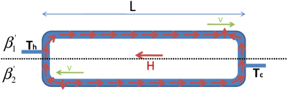
Figure 2: (Color online) Magnetocaloritronic cooling can be realized by moving domain walls between two regions with different viscous coupling $\beta^{{}^{\prime}}$. The cyclic motion of the domain walls is maintained by the rotating clockwise magnetic field (along a horizontally elongated elliptical trajectory) in sync with the domain walls steadily circulating clockwise; this process is analogous to a pump which produces a dc heat flow between the cold ($T_{c}$) and hot ($T_{h}$) junctions. The analogy to the thermoelectric cooling based on p- and n-type couples [2] can be best seen when $p_{1}^{{}^{\prime}}\beta_{1}^{{}^{\prime}}=-p_{2}^{{}^{\prime}}\beta_{2}^{{}^{\prime}}$.

It is customary to describe the efficiency of thermoelectric circuits by a material figure of merit $Z=\Pi^{2}\sigma/T^{2}\kappa$ corresponding to the maximum achievable temperature difference $\sim ZT^{2}$. In most circumstances, a dimensionless figure, $ZT$, is quoted and it corresponds to the relative temperature difference. Let us formulate an analog of figure of merit for magnetocaloritronic device. We consider the case of relatively small temperature gradients $T_{h}-T_{c}\ll T_{h}$. In order to maintain the domain wall motion, we have to perform the work $2MHL\mathcal{A}$ per one pass and all this work is eventually dissipated, where $H$ is the applied field along the magnetic wires and $\mathcal{A}$ is the cross-section of the wire. From Eq. (3), we find that in the absence of temperature bias, the domain wall induces the heat current:

$$j_{\mbox{tr}}=\dfrac{\mathcal{O}_{XT}}{\mathcal{O}_{T}}\dfrac{2MH}{L}\>.$$ (10)

For simplicity, we suppose that the charge current can not flow in the device in Fig. 2 (e.g. due to a breaking point or upper and lower parts could be different p- and n-type semiconductors, whose junctions block the current flow). Supposing that the dissipated work is equally distributed between the reservoirs, the externally induced heat flow from the cold/hot reservoir per one wire then becomes:

$$\begin{array}[]{c}j_{q}^{\mbox{cold}}=\dfrac{T_{h}-T_{c}}{TL\mathcal{O}_{T}}+\dfrac{\mathcal{O}_{XT}}{\mathcal{O}_{T}}\dfrac{2MH}{L}+HM\dot{X}\>,\\ j_{q}^{\mbox{hot}}=\dfrac{T_{h}-T_{c}}{TL\mathcal{O}_{T}}+\dfrac{\mathcal{O}_{XT}}{\mathcal{O}_{T}}\dfrac{2MH}{L}-HM\dot{X}\>.\end{array}$$ (11)

Because the domain wall cooling is proportional to the magnetic field and dissipative heating is proportional to the magnetic field squared, the maximum decrease in the junction temperature is obtained at an optimal magnetic field. This situation is similar to thermoelectric cooling in which the Peltier cooling is proportional to current and Joule heating is proportional to the current squared, leading to existence of an optimal current. From Eq. (11), the maximum temperature difference that the domain wall motion can maintain becomes:

$$(T_{h}-T_{c})^{\mbox{max}}=\dfrac{T\mathcal{O}_{XT}^{2}}{2\mathcal{O}_{X}\mathcal{O}_{T}}\>.$$

We can finally introduce the figure of merit for the magnetocaloritronic cooling:

$$TZ_{\mbox{mc}}=\dfrac{\mathcal{O}_{XT}^{2}}{\mathcal{O}_{X}\mathcal{O}_{T}}=\dfrac{1}{\dfrac{\alpha sWL\bar{\zeta}}{2p^{{}^{\prime}2}\beta^{{}^{\prime}2}}-1}\>,$$ (12)

where the last part of the equation is written for a domain wall described by microscopic Eqs. (4), (5) and (6). Notice that $TZ_{\mbox{mc}}>0$ as it follows from the thermodynamic inequalities $\mathcal{O}_{T}\geq 0$ and $\mathcal{O}_{X}\geq 0$ which guarantee that the entropy production in Eqs. (2) is always positive. It is also worthwhile to note that the efficiency $TZ_{\mbox{mc}}$ becomes infinite when $\bar{\zeta}=2p^{{}^{\prime}2}\beta^{{}^{\prime}2}/WL\alpha s$ which corresponds exactly to the lower bound of the thermal resistivity [10], $\zeta=\eta_{\zeta}(\partial_{x}\mathbf{m})^{2}$ with $\eta_{\zeta}=\beta^{\prime 2}p^{\prime 2}/\alpha s$, averaged over the Walker ansatz.

Above, we only considered dissipation in the lower wire in Fig. 2. Consideration of the upper wire does not change our results when the upper wire is mirror symmetric to the lower with $p_{1}^{{}^{\prime}}\beta_{1}^{{}^{\prime}}=-p_{2}^{{}^{\prime}}\beta_{2}^{{}^{\prime}}$ (e.g. we do not see any principal contradictions in existence of negative $\beta^{{}^{\prime}}$). In a different scenario when $\beta_{1}^{{}^{\prime}}=0$ and $\beta_{2}^{{}^{\prime}}\neq 0$, it is possible to minimize the effect of dissipation in the upper part by keeping the upper wire disconnected from the cold/hot junction most of the time apart from the moments when the domain wall moves through.

It is interesting to see that a system in Fig. 2 made of p- and n-type semiconductors for upper and lower parts will have opposite $p\beta$ in those parts leading to a device that can generate electrical power from a rotating magnetic field in accordance with Eqs. (3).

At last, we recover the well known expressions for the maximum coefficient of performance ($COP$) [29] written for the magnetocaloritronic cooling and heating:

$$COP_{\mbox{heat}}=\dfrac{j_{q}^{\mbox{hot}}}{2HM\dot{X}}=\dfrac{T_{h}}{T_{h}-T_{c}}\dfrac{\sqrt{1+TZ_{\mbox{mc}}}-T_{c}/T_{h}}{\sqrt{1+TZ_{\mbox{mc}}}+1}\>,$$ (13)

$$COP_{\mbox{cool}}=\dfrac{j_{q}^{\mbox{cold}}}{2HM\dot{X}}=\dfrac{T_{c}}{T_{h}-T_{c}}\dfrac{\sqrt{1+TZ_{\mbox{mc}}}-T_{h}/T_{c}}{\sqrt{1+TZ_{\mbox{mc}}}+1}\>,$$ (14)

where we maximized the above equations with respect to $H$ at a fixed temperature bias. The Carnot efficiency is recovered when $TZ_{\mbox{mc}}\rightarrow\infty$.

Using Eq. (7), we can express the magnetocaloritronic figure of merit via the thermoelectric figure of merit:

$$TZ_{\mbox{mc}}=\dfrac{1}{\dfrac{\alpha sWL}{ZT\left[\beta^{{}^{\prime}}\wp_{S}(1-\wp^{2})\hbar/2e\right]^{2}\sigma}-1}\>,$$

which gives a very small number $Z_{\mbox{mc}}\approx 10^{-7}Z$ for a typical domain wall in a Py wire at room temperature with $L=2W=100\>\mbox{nm}$. Much more pronounced cooling effect could be seen in MnSi below $30$K for which we obtain $Z_{\mbox{mc}}\approx 10^{-3}Z$ (MnSi parameters are taken to be the same with Ref. [10]). We speculate that one can achieve better efficiencies using the ferromagnetic insulators in which the heat transferred by spin waves will better couple to the texture dynamics in the absence of dissipation related to the electron-hole continuum. Large viscous $\beta$-like coupling with domain wall motion have recently been predicted for dirty (Ga,Mn)As [25] which can lead to larger $TZ_{\mbox{mc}}$ according to Eq. (12). Note that the best materials available today for devices that operate near room temperature have a $ZT$ of about $1\div 2$ [2, 30].

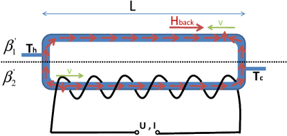
Figure 3: (Color online) Magnetocaloritronic power generation can be realized by maintaining cyclic motion of domain walls between two regions with different viscous coupling $\beta^{{}^{\prime}}$. The cyclic motion of the domain walls can be maintained by the temperature gradient when $p^{{}^{\prime}}\beta^{{}^{\prime}}$ has opposite sign for the upper and lower parts. Alternatively, when $\beta_{1}^{{}^{\prime}}=0$, a small magnetic field $H_{\mbox{back}}$ can return the domain walls to the hot junction. The power (useful work) is extracted from a solenoid encircling one of the wires.

4 Magnetocaloritronic power generation

Thermoelectric devices find numerous applications as voltage generators [2]. In this section, continuing the analogy between the thermoelectric devices and the magnetocaloritronic devices, we will show how power and useful work can be generated magnetocaloritronically. The device depicted in Fig 3 once again contains two regions with different viscous coupling $\beta^{{}^{\prime}}$. The temperature gradient propels domain walls in the lower part with $\beta^{{}^{\prime}}\neq 0$ as it follows from Eq. 3 while in the upper part with $\beta^{{}^{\prime}}=0$ the domain walls are inert to the temperature gradient and move due to the presence of a very small magnetic field $H_{\mbox{back}}$. As an alternative, one could also consider the mirror symmetric case with $p_{1}^{{}^{\prime}}\beta_{1}^{{}^{\prime}}=-p_{2}^{{}^{\prime}}\beta_{2}^{{}^{\prime}}$ and with an additional solenoid encircling the upper wire.

Let us calculate the ratio of the useful power to the losses (efficiency) for a magnetocaloritronic device. We again suppose that the charge current can not flow in the device in Fig. 3 (e.g. due to a breaking point or upper and lower parts could be different p- and n-type semiconductors also blocking the current flow) and we consider the case of relatively small temperature gradients $T_{h}-T_{c}\ll T_{h}$. The dissipation due to domain wall motion $2MHL\mathcal{A}$ is again evenly distributed along the wire and between reservoirs as we make similar assumptions with the previous section. The losses then appear due to the finite heat conductivity $j_{q}^{\mbox{cond}}=(T_{h}-T_{c})/TL\mathcal{O}_{T}$ and due to domain wall motion. The motion of domain wall through the solenoid will lead to electromotive force in the solenoid $U=8\pi M\mathcal{A}N\dot{X}/L$ where $N$ is the number of loops in the solenoid and $\dot{X}$ is the average velocity of the domain wall that can be found from Eq. (3) with the magnetic field inside of the solenoid $H=4\pi IN/L$. One can write the following expression for the useful power:

$$UI=2M\mathcal{A}\dot{X}H\>,$$

which, as in the previous section, suggests the existence of the optimal $H$ for the maximum power outcome. We can finally recover the well known expression for the maximum thermoelectric efficiency of power generation [29] written for the magnetocaloritronic power efficiency. By maximizing the ratio of the power (work) $UI$ to the losses (heat absorbed at the hot end given by Eq. (11)) at a fixed temperature bias for the device in Fig. 3, we obtain:

$$\eta=\dfrac{UI}{j_{q}^{\mbox{hot}}\mathcal{A}}=\dfrac{T_{h}-T_{c}}{T_{h}}\dfrac{\sqrt{1+TZ_{\mbox{mc}}}-1}{\sqrt{1+TZ_{\mbox{mc}}}+T_{c}/T_{h}}\>.$$ (15)

As expected, the magnetocaloritronic figure of merit also contains information about the efficiency of the magnetocaloritronic device working as a power (useful work) generator. The Carnot efficiency is once again recovered when $TZ_{\mbox{mc}}\rightarrow\infty$.

In the above estimates, we again considered dissipation only in the lower wire in Fig. 3. Consideration of the upper wire does not change our results when the upper wire contains an extra solenoid and is mirror symmetric to the lower with $p_{1}^{{}^{\prime}}\beta_{1}^{{}^{\prime}}=-p_{2}^{{}^{\prime}}\beta_{2}^{{}^{\prime}}$. In the scenario when $\beta_{1}^{{}^{\prime}}=0$ and $\beta_{2}^{{}^{\prime}}\neq 0$, a small magnetic field $H_{\mbox{back}}$ returns the domain walls to the hot junction and we minimize the effect of dissipation in the upper part by keeping the upper wire disconnected from the hot junction most of the time apart from the moments when the domain wall moves through.

5 Conclusions

We introduced and described the magnetocaloritronic circuit element using recently formulated phenomenological theory of thermoelectric spin transfer [10]. The velocity of domain wall in such a circuit element in response to magnetic field, charge current and energy flow is calculated. We also derive the most general form of phenomenological equations describing dynamics of a domain wall in response to the magnetic field, applied voltage and temperature biases. We conclude that such hybrid device combines functionalities of thermoelectric and spintronic devices.

As an example of some of the possible functionalities of the circuit element, we propose a realization of magnetocaloritronic cooling and power generation. We further study the efficiency of the magnetocaloritronic cooling and power generation which leads us to the introduction of the magnetocaloritronic figure of merit by analogy to the thermoelectric figure of merit. Our estimates of the magnetocaloritronic figure of merit for Py and MnSi give very small numbers unusable for applications. However, we speculate that one can achieve better efficiencies using the ferromagnetic insulators in which the heat transferred by spin waves will better couple to the texture dynamics in the absence of dissipation related to the electron-hole continuum.

This work was supported in part by the Alfred P. Sloan Foundation, DARPA and NSF under Grant No. DMR-0840965.

References

- Pecharsky and Gschneidner, Jr. [1999] V. K. Pecharsky and K. A. Gschneidner, Jr., J. Magn. Magn. Mater. 200, 44 (1999).
- DiSalvo [1999] F. J. DiSalvo, Science 285, 703 (1999).
- Ohta et al. [2007] H. Ohta, S. Kim, Y. Mune, T. Mizoguchi, K. Nomura, S. Ohta, T. Nomura, Y. Nakanishi, Y. Ikuhara, M. Hirano, et al., Nature Mater. 6, 129 (2007).
- Murphy et al. [2008] P. Murphy, S. Mukerjee, and J. Moore, Phys. Rev. B 78, 161406 (2008).
- Sales [2002] B. C. Sales, Science 295, 1248 (2002).
- Hochbaum et al. [2008] A. I. Hochbaum, R. Chen, R. D. Delgado, W. Liang, E. C. Garnett, M. Najarian, A. Majumdar, and P. Yang, Nature 451, 163 (2008).
- Boukai et al. [2008] A. I. Boukai, Y. Bunimovich, J. Tahir-Kheli, J.-K. Yu, W. A. Goddard III, and J. R. Heath, Nature 451, 168 (2008).
- Hatami et al. [2007] M. Hatami, G. E. W. Bauer, Q. Zhang, and P. J. Kelly, Phys. Rev. Lett. 99, 066603 (2007).
- Hatami et al. [2009] M. Hatami, G. E. W. Bauer, Q. Zhang, and P. J. Kelly, Phys. Rev. B 79, 174426 (2009).
- Kovalev and Tserkovnyak [2009] A. A. Kovalev and Y. Tserkovnyak, Phys. Rev. B 80, 100408 (2009).
- Bauer et al. [unpublished] G. E. W. Bauer, S. Bretzel, A. Brataas, and Y. Tserkovnyak, arXiv:0910.4712 (unpublished).
- Berger [1996] L. Berger, Phys. Rev. B 54, 9353 (1996).
- Slonczewski [1996] J. C. Slonczewski, J. Magn. Magn. Mater. 159, L1 (1996).
- Yamaguchi et al. [2004] A. Yamaguchi, T. Ono, S. Nasu, K. Miyake, K. Mibu, and T. Shinjo, Phys. Rev. Lett. 92, 077205 (2004).
- Hayashi et al. [2006] M. Hayashi, L. Thomas, Y. B. Bazaliy, C. Rettner, R. Moriya, X. Jiang, and S. S. P. Parkin, Phys. Rev. Lett. 96, 197207 (pages 4) (2006).
- Hayashi et al. [2007] M. Hayashi, L. Thomas, C. Rettner, R. Moriya, and S. S. P. Parkin, Nat. Phys. 3, 21 (2007).
- Tatara et al. [2008] G. Tatara, H. Kohno, and J. Shibata, Phys. Rep. 468, 213 (2008).
- Ralph and Stiles [2008] D. Ralph and M. Stiles, J. Magn. Magn. Mater. 320, 1190 (2008).
- Tserkovnyak et al. [2008] Y. Tserkovnyak, A. Brataas, and G. E. Bauer, J. Magn. Magn. Mater. 320, 1282 (2008).
- Parkin et al. [2008] S. S. P. Parkin, M. Hayashi, and L. Thomas, Science 320, 190 (2008).
- Barnes and Maekawa [2007] S. E. Barnes and S. Maekawa, Phys. Rev. Lett. 98, 246601 (2007).
- Tserkovnyak and Mecklenburg [2008] Y. Tserkovnyak and M. Mecklenburg, Phys. Rev. B 77, 134407 (2008).
- Duine [2008] R. A. Duine, Phys. Rev. B 77, 014409 (2008).
- Saslow [2007] W. M. Saslow, Phys. Rev. B 76, 184434 (2007).
- Hals et al. [2009] K. M. D. Hals, A. K. Nguyen, and A. Brataas, Phys. Rev. Lett. 102, 256601 (2009).
- Tserkovnyak and Wong [2009] Y. Tserkovnyak and C. H. Wong, Phys. Rev. B 79, 014402 (2009).
- Schryer and Walker [1974] N. L. Schryer and L. R. Walker, J. Appl. Phys. 45, 5406 (1974).
- Li and Zhang [2004] Z. Li and S. Zhang, Phys. Rev. B 70, 024417 (2004).
- Mahan [1997] G. Mahan, Solid State Phys. 51, 81 (1997).
- Harman et al. [2005] T. Harman, M. Walsh, B. Laforge, and G. Turner, J. Electron. Mater. 34, L19 (2005).