Existence, Stability, and Scattering of Bright Vortices in the Cubic-Quintic Nonlinear Schrödinger Equation

Abstract

We revisit the topic of the existence and azimuthal modulational stability of solitary vortices (alias vortex solitons) in the two-dimensional (2D) cubic-quintic nonlinear Schrödinger equation. We develop a semi-analytical approach, assuming that the vortex soliton is relatively narrow, and thus splitting the full 2D equation into radial and azimuthal 1D equations. A variational approach is used to predict the radial shape of the vortex soliton, using the radial equation, yielding results very close to those obtained from numerical solutions. Previously known existence bounds for the solitary vortices are recovered by means of this approach. The 1D azimuthal equation of motion is used to analyze the modulational instability of the vortex solitons. The semi-analytical predictions – in particular, that for the critical intrinsic frequency of the vortex soliton at the instability border – are compared to systematic 2D simulations. We also compare our findings to those reported in earlier works, which featured some discrepancies. We then perform a detailed computational study of collisions between stable vortices with different topological charges. Borders between elastic and destructive collisions are identified.

I Introduction

The cubic-quintic nonlinear Schrödinger (CQNLS) equation is used to model a variety of physical settings. In scaled units, the CQNLS equation takes the following form:

$$i\frac{\partial\Psi}{\partial t}+\nabla^{2}\Psi+\left|\Psi\right|^{2}\!\Psi-\left|\Psi\right|^{4}\!\Psi=0,$$ (1)

where $\Psi(x,y,t)$ is the complex wave function, $\nabla^{2}$ is the two-dimensional (2D) Laplacian, and the last two terms represent, respectively, the focusing cubic and defocusing quintic nonlinearities. The CQNLS equation emerges in models of light propagation in diverse optical media, such as non-Kerr crystals PTS , chalcogenide glasses CQglass1 ; CQglass2 , organic materials CQorganic , colloids colloid1 ; colloid2 , dye solutions dye , and ferroelectrics ferroelectric . It has also been predicted that this complex nonlinearity can be synthesized by means of a cascading mechanism cascading . It should be noticed that, in the optics models, evolution variable $t$ is not time, but rather the propagation distance.

The competition of the focusing (cubic) and defocusing (quintic) nonlinear terms is the key feature of the CQNLS model, which allows for the existence of stable multidimensional structures which would be unstable in the focusing cubic nonlinear Schrödinger (NLS) equation. In particular, the CQNLS equation supports solitary vortices (alias vortex solitons) in 2D and 3D geometries. These are ring-shaped structures which carry a rotational angular phase. The respective integer winding number in the vortex is referred to as its topological charge (alias vorticity), $m$. An example of a stable solitary vortex is depicted in Fig. 1.

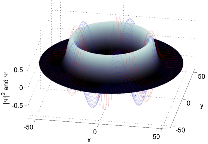
Figure 1: (Color online) An example of a vortex soliton with charge $m=5$ and frequency $\Omega=0.16$, found as a numerical solution to the CQNLS equation. The height of the profiles represents the value of the wave function. The gray profile displays the squared absolute value, while the dark (blue) and light (red) meshes represent the real and imaginary parts, respectively.

It is well known that the cubic NLS equation supports “dark” (delocalized) and “bright” (localized) vortices, with the self-defocusing and focusing signs of the nonlinearity, respectively. Dark vortices of unitary charge are stable, while higher-order ones are unstable, splitting into unitary eddies Fetter . On the other hand, the “bright” modes (vortex solitons) are always azimuthally unstable in the framework of the cubic equation or its counterpart with the saturable nonlinearity Skryabin , which leads to the breaking of the vortex soliton into a number of fragments depending on the charge NLSxMI ; Torner . The addition of a periodic potential to the cubic NLS equation may stabilize vortex solitons of a different type, which are built (in the simplest case) as a chain of four peaks with the phase circulation corresponding to integer vorticity $m$ pu99 ; Baizakov ; Yang ; herring08 ; Thawatchai . An example of the azimuthal breakup of an unstable vortex is displayed in Fig. 2.

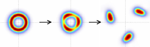
Figure 2: (Color online) An example of the evolution of the vortex soliton with charge $m=4$ in the CQNLS equation, exhibiting breakup (left to right) due to the azimuthal modulational instability. Shown is the intensity (squared absolute value of the wave function) at consecutive moments of time, from left to right. The numerical method and parameters are presented in Sec. V.

In contrast to the cubic NLS, the CQNLS can support stable solitary vortices. For the first time, this remarkable fact was discovered “empirically” in simulations of the 2D CQNLS equation AMIxCQNLSxOLD , and later was investigated in detail in a more rigorous form in Refs. AMIxCQNLSxSHORT ; AMIxCQNLSxLONG . Moreover, three-dimensional solitons with embedded vorticity $m=1$ also have their stability region in the 3D CQNLS equationPRL (see also reviews AMIxCQNLSxMID ; Torner ). Stable vortex solitons may find their potential applications in the design of all-optical data-processing schemes. In that respect, knowing the growth rates of unstable modes is also important, because, if the rates are small enough, the vortices may be considered as practically stable ones, as they will not exhibit an observable instability over relevant propagation distances.

One of objectives of this paper is to revisit the topic of the azimuthal modulational stability of solitary-vortex solutions in the 2D CQNLS equation. As mentioned above, numerous studies of this problem have already been published AMIxCQNLSxOLD ; AMIxCQNLSxSHORT ; AMIxCQNLSxMID ; AMIxCQNLSxLONG ; AMIxCQNLSxNEW . The aim of the analysis was to find a critical value ($\Omega_{\mbox{\scriptsize st}}$) of the intrinsic frequency of the vortex [for its exact definition see Eqs. (2) and (3) below], above which the vortices with a given value of the topological charge are stable. In Ref. AMIxCQNLSxOLD , 2D azimuthally stable vortices with $m=1$ were shown to exist. It was found that the slope of the vortex’ profile at the pivotal point peaked at a specific value of $\Omega$, which was considered as the critical frequency, $\Omega_{\mbox{\scriptsize st}}(m=1)\approx 0.145$, while the vortices, with all values of $m$, exist at $\Omega<\Omega_{\mbox{\scriptsize max}}^{\mbox{\scriptsize 1D}}=3/16\equiv 0.1875$ (at $\Omega=\Omega_{\mbox{\scriptsize max}}^{\mbox{\scriptsize 1D}}$, the radius of the vortex diverges, i.e., the “bright” vortex goes over into a “dark” one). The same value, $\Omega_{\mbox{\scriptsize max}}^{\mbox{\scriptsize 1D}}$ is simultaneously the largest one up to which exact soliton solutions exist in the 1D version of the CQNLS equation Bulgaria . In work AMIxCQNLSxOLD , a variational approach (VA) was developed for 2D vortex solitons, yielding results similar to those obtained in the numerical form. Full 2D simulations of the CQNLS equation reported in Ref. AMIxCQNLSxOLD had confirmed that vortices with $\Omega_{\mbox{\scriptsize st}}<\Omega<\Omega_{\mbox{\scriptsize max}}^{\mbox{\scriptsize 1D}}$ were indeed stable, while those with $0<\Omega<\Omega_{\mbox{\scriptsize st}}$ were not.

Works AMIxCQNLSxSHORT ; AMIxCQNLSxMID ; AMIxCQNLSxLONG employed a more rigorous approach. They introduced small perturbations around the 2D vortex soliton and solved the resulting eigenvalue problem numerically. In this way, the critical frequencies were found as $\Omega_{\mbox{\scriptsize st}}(m=1)\approx 0.16$ and $\Omega_{\mbox{\scriptsize st}}(m=2)\approx 0.17$. Also, in Ref. Victor08 , using the Gagliardo-Nirenberg and Hölder inequalities together with Pohozaev identities, is was shown that the eigenvalues generated by the CQNLS equation possess an upper cutoff value.

In Ref. AMIxCQNLSxNEW , 2D perturbations were considered too. Through an extensive analysis, the problem was transformed into finding, by means of numerical methods, zeros of respective Evans functions for a set of ordinary differential equations (ODEs). In this way, the existence of azimuthally stable vortices of all integer values of $m$ was predicted (in Refs. AMIxCQNLSxSHORT and AMIxCQNLSxOLD , the stability regions for $m\geq 3$ were not identified, as they are extremely small). The predictions for the critical frequencies reported in Ref. AMIxCQNLSxNEW , which are somewhat different from those in Refs. AMIxCQNLSxSHORT and AMIxCQNLSxOLD , are shown in Table 2.

The present work aims to undertake an additional study of the stability of vortices in the CQNLS equation for two reasons. Firstly, the previous studies demonstrated some (relatively small, but not negligible) disagreement in the predictions of the critical frequency. Therefore, since we will use a different approach, our results may help in comparing and verifying the previous findings. Secondly, although in Ref. AMIxCQNLSxOLD 2D simulations were performed for the vortices, this was only done for $m=1$, and longer simulations later showed that some vortices which were originally concluded to be stable turned out to be eventually unstable AMIxCQNLSxSHORT . Therefore, stability results from additional 2D numerical simulations are needed for comparison with various predictions of the stability. In fact, our numerical results will illustrate that the predictions of Ref. AMIxCQNLSxNEW are the most accurate ones. In parallel to extensive direct simulations, we elaborate a semi-analytical methodology, following the lines of previous studies of the azimuthal modulational instability of vortices in the cubic NLS equation NLSxMI . The approximation amounts to splitting the full 2D equation into effectively one-dimensional radial and azimuthal equations. The former equation is used to compute the radial shape of the soliton by means of a VA to find an analytic approximation to the profile, which is then used as an initial condition to a numerical optimization routine to find the numerically ‘exact’ profile. The closeness between the numerically computed profiles and the VA approximation testify to the good accuracy of the VA. The analysis of the azimuthal equation makes it possible to predict the threshold of the onset of the splitting instability of the vortex soliton. Our results predicting the growth rates of individual azimuthal modes of unstable vortices match full simulations very well, but the predictions for the critical frequency are less accurate, when compared to the simulations. This semi-analytical technique may be quite relevant for applications in other 2D models.

Another objective of the work is to study, by means of systematic simulations, collisions between stable vortices. Except for few examples reported in Ref. AMIxCQNLSxOLD , this problem was not studied before.

The paper is organized as follows. In Sec. 2 we derive an approximate analytical description of the vortex profile by first finding an analytical asymptotic approximation to it, which is then employed as the ansatz on which the VA is based. In Sec. 3 we use the variational ansatz as the initial guess, to generate numerically exact vortex profiles by dint of a nonlinear optimization routine. We then compare the numerical profiles with the variational ansatz to show its accuracy. In Sec. 4 we derive an approximate 1D equation for the dynamics along the azimuthal direction. A linear stability analysis is subsequently performed to find stability criteria and growth rates of unstable modes within the framework of the azimuthal equation. In Sec. 5 we present full 2D simulations of the vortices, and the respective results for their stability. These results are compared to our predictions, as well as to the predictions produced by previous works. In Sec. 6, we use direct simulations to explore collisions between stable vortices in detail. In particular, these studies allow us to identify a border between quasi-elastic and destructive collisions. Finally, in Sec. 7, we summarize our findings and formulate concluding remarks.

II Approximate Analytical Profiles of Steady-State Vortices

A steady-state vortex solution to Eq. (1) is looked for as

$$\Psi(r,\theta,t)=f(r)\,A(\theta,t),$$ (2)

where real function $f(r)$ is a stationary radial profile with azimuthal dependence given by

$$A(\theta,t)=e^{i(m\theta+\Omega t)},$$ (3)

with topological charge $m$ and frequency $\Omega$. Analytical solutions being not available for the profile $f(r)$, we begin the study by finding an approximate analytic expression for $f(r)$ and identifying its existence bounds. As shown below in Sec. III, the predicted profile is very close to the true solution, therefore it can be used to predict the existence and stability regions of the vortex solitons. The developed analytical method is quite general and may be applied to other physically relevant equations.

II.1 The Asymptotic Vortex Profile

Inserting expression (2) into the underlying equation (1) yields the following ODE for the radial profile of the vortex with charge $m$:

$$\frac{1}{r}\frac{d}{dr}\left(r\frac{df}{dr}\right)-\left(\Omega+\frac{m^{2}}{r^{2}}\right)f(r)+f^{3}(r)-f^{5}(r)=0.$$ (4)

If we assume that the vortex takes the form of a relatively narrow ring with a large radius, then, in the region of interest, variable $r$ may be approximately replaced by a constant, $r_{c}\gg 1$, which we take to be the value of $r$ at a point where the radial profile attains its maximum. Since we assume $r_{c}$ to be large, in the lowest approximation we neglect the $1/r_{c}$ term in the Laplacian. An obvious consequence of dropping this term is that the approximate profiles which we are going to derive will be less accurate for smaller values of $r_{c}$, see Sec. III.

Under the large-radius assumption, Eq. (4) becomes

$$\frac{d^{2}\!f}{dr^{2}}-\Omega^{\ast}\,f(r)+f^{3}(r)-f^{5}(r)=0,$$ (5)

$$\Omega^{\ast}\equiv\Omega+m^{2}/r_{c}^{2}.$$ (6)

For a relatively narrow ring, one can treat Eq. (5) as if $r\in(-\infty,+\infty)$, in which case the equation has a well-known 1D analytical solution for the soliton Bulgaria ; CQNLS1DSOL :

$$f_{\mbox{\scriptsize asy}}^{2}(r)=\frac{4\Omega^{\ast}}{1+\sqrt{1-(16/3)\Omega^{\ast}}\,\cosh\left(2\sqrt{\Omega^{\ast}}\,(r-r_{c})\right)}.$$ (7)

As mentioned above, this solution exists for $0<\Omega^{\ast}<\Omega_{\mbox{\scriptsize max}}^{\mbox{\scriptsize 1D}}\equiv 3/16$. At point $\Omega^{\ast}=3/16$, the solution degenerates into a constant, $f(r)=f_{0}\equiv\sqrt{3/4}$. The family of solutions (7) parameterized by $\Omega^{\ast}$ is depicted in Fig. 3.

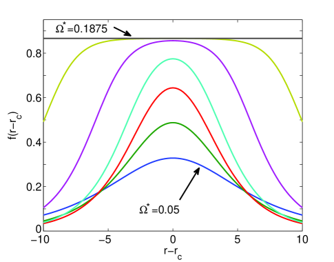
Figure 3: (Color online) A set of solutions (7) for $\Omega^{\ast}=0.05,0.1,0.15,0.18,0.1874,0.1874999,0.1875$ are shown from bottom to top. As $\Omega^{\ast}$ increases, the profile flattens out, and it degenerates into a constant at $\Omega=\Omega^{\ast}$.

To obtain a closed-form analytical approximation, it is now necessary to find an expression for the radius of the profile, $r_{c}$, for given frequency $\Omega$. To this end, we will use the VA, and will then compare the results with numerically found profiles.

II.2 The Variational Approach

To apply the VA, we use the Lagrangian density corresponding to the CQNLS equation:

$$\mathcal{L}=\frac{i}{2}\left(\Psi\Psi_{t}^{\ast}-\Psi^{\ast}\Psi_{t}\right)+|\Psi_{r}|^{2}+r^{-2}|\Psi_{\theta}|^{2}-\frac{1}{2}|\Psi|^{4}+\frac{1}{3}|\Psi|^{6},$$ (8)

where the subscripts denote partial derivatives. Inserting here expression (2), to be used as a factorized ansatz, yields

$$\mathcal{L}=\left(\Omega+\frac{m^{2}}{r^{2}}\right)f^{2}(r)+\left(\frac{df}{dr}\right)^{2}-\frac{1}{2}f^{4}(r)+\frac{1}{3}f^{6}(r).$$ (9)

The integration of density (9) gives rise to the full Lagrangian:

$$L\equiv 2\pi\int_{0}^{\infty}\mathcal{L}(r)dr=2\pi\left(\Omega\,C_{1}+C_{2}+m^{2}\,C_{3}-\frac{1}{2}\,C_{4}+\frac{1}{3}\,C_{5}\right),$$ (10)

where

$$C_{1} \equiv\int_{0}^{\infty}f^{2}(r)r\,dr, \qquad C_{2} \equiv\int_{0}^{\infty}\left(\frac{df}{dr}\right)^{2}r\,dr,$$

$$C_{3} \equiv\int_{0}^{\infty}\!f^{2}(r)\,\frac{dr}{r}, \qquad C_{4} \equiv\int_{0}^{\infty}\!f^{4}(r)r\,dr,$$ (11)

$$C_{5} \equiv\int_{0}^{\infty}\!f^{6}(r)r\,dr.$$

Next, we use the asymptotic approximate profile (7) as an ansatz for radial profile, treating $\Omega^{\ast}$ and $r_{c}$ in Eq. (7) as variational parameters. Inserting expression (7) into the integral terms in the Lagrangian, and again making use of the large-radius approximation yields

$$C_{1} \approx 2\sqrt{3}\,T\,r_{c},\quad C_{2}\approx r_{c}\left[\frac{3}{8}\sqrt{\Omega^{\ast}}-\sqrt{3}\,T\,\left(\frac{3}{16}-\Omega^{\ast}\right)\right],$$

$$C_{3} \approx\frac{2\sqrt{3}\,T}{r_{c}},\quad C_{4}\approx-3\,r_{c}\left[\sqrt{\Omega^{\ast}}-\frac{\sqrt{3}}{2}\,T\right],$$ (12)

$$C_{5} \approx-r_{c}\left[\frac{27}{8}\sqrt{\Omega^{\ast}}-3\sqrt{3}\,T\left(\frac{9}{16}-\Omega^{\ast}\right)\right],$$

where

$$T\equiv\mbox{arctanh}\left[\sqrt{\frac{3}{16\Omega^{\ast}}}-\sqrt{\frac{3}{16\Omega^{\ast}}-1}\right].$$ (13)

The respective static Euler-Lagrange equations, ${\partial L}/{\partial r_{c}}=0$ and ${\partial L}/{\partial\Omega^{\ast}}=0$, yield, respectively, equation

$$r_{c}=m\left(\Omega-\frac{3}{16}+\frac{\sqrt{3\Omega^{\ast}}}{8T}\right)^{-1/2},$$ (14)

and the other one which is equivalent to Eq. (6). Eliminating $r_{c}$ from these equations, one concludes that $\Omega^{\ast}$ is, for a chosen value of $\Omega$, a solution to the following equation,

$$\Omega=\frac{\Omega^{\ast}}{2}+\frac{3}{32}-\frac{\sqrt{3\Omega^{\ast}}}{16T}\equiv G(\Omega^{\ast}).$$ (15)

This yields the final form of the vortex radial profile, as predicted by the VA:

$$f_{\mbox{\scriptsize va}}^{2}(r)=\frac{4\Omega^{\ast}}{1+\sqrt{1-(16/3)\Omega^{\ast}}\,\cosh\left(2\sqrt{\Omega^{\ast}}\,(r-r_{c}^{\mbox{\scriptsize va}})\right)},$$ (16)

$$r_{c}^{\mbox{\scriptsize va}}\equiv\frac{m}{\sqrt{\Omega^{\ast}-G(\Omega^{\ast})}}.$$ (17)

Finally, the transcendental equation (15), together with Eq. (13), was solved numerically by means of a simple bisection method with a tolerance of $10^{-15}$.

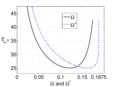
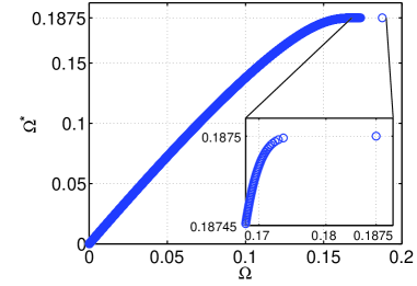
Figure 4: (Color online) Top: The vortex’ radius, as predicted by the variational approximation, $r_{c}^{\mbox{\scriptsize va}},$ versus $\Omega=G(\Omega^{\ast})$, and $\Omega^{\ast}$, for $m=5$. Bottom: The values of $\Omega=G(\Omega^{\ast})$ vs. $\Omega^{\ast}$, see Eq. (6). $G(\Omega^{\ast})$ was evaluated over interval $\Omega^{\ast}\in\left[0.01,0.1875\right]$ with step $\Delta\Omega^{\ast}=0.00001$.

In Fig. 4 we show $r_{c}^{\mbox{\scriptsize va}}$ versus $\Omega$ and $\Omega^{\ast}$ for $m=5$, along with relationship (15). We see that, with the increase of $\Omega$, the radius of the vortex starts from very large values (infinite at $\Omega=0$), decreases until it reaches a minimum value, and then increases rapidly (it becomes infinite once again at $\Omega=\Omega_{\mbox{\scriptsize max}}^{\mbox{\scriptsize 2D}}$). We also see that the relationship between $\Omega$ and $\Omega^{\ast}$ does not depend on charge $m$, and that $\Omega\rightarrow 3/16\$as $\Omega^{\ast}\rightarrow 0.1875$ (the apparent gap near the right edge of the plot is due to the sensitivity of the relationship, which we discuss below).

II.3 Existence Bounds for the Two-Dimensional Vortex Profiles

From numerical investigations performed in Refs. AMIxCQNLSxOLD and AMIxCQNLSx2D3D , the existence border for the two-dimensional CQNLS equation vortex solution was found to be $\left(\Omega_{\mbox{\scriptsize max}}^{\mbox{\scriptsize 2D}}\right)_{\mathrm{num}}\approx 0.180$, while, as said above, the analytical limit, which is identical for 1D and 2D equations, is $\Omega_{\mbox{\scriptsize max}}^{\mbox{\scriptsize 2D}}=\Omega_{\mbox{\scriptsize max}}^{\mbox{\scriptsize 1D}}=3/16=0.1875.$ The discrepancy may be explained by the sensitivity of relationship (15) between $\Omega$ and $\Omega^{\ast}$, as produced by the variational approximation. From Eqs. (15) and (13) we see that, as $\Omega^{\ast}\rightarrow 3/16$, $T\rightarrow\infty$, and so $\Omega=G(\Omega^{\ast})\rightarrow\Omega^{\ast}/2+3/32=3/16$, in accordance with the exact result. However, as seen in the right panel of Fig. 4, the relationship between $\Omega$ and $\Omega^{\ast}$ seems to be extremely sensitive near this limit (see the inset in the right panel of Fig. 4). This sensitivity can also be observed in Table 1, where some values of $\Omega^{\ast}$ and the corresponding $G(\Omega^{\ast})=\Omega$ are given. It is clearly seen that one quickly approaches the limit of machine double precision for $\Omega^{\ast}$ as $\Omega\rightarrow 0.1875$.

$\Omega^{*}$	$\Omega=G(\Omega^{*})$
0.1874	0.1664…
0.187499	0.1736…
0.187499999	0.1783…
0.187499999999	0.1806…
0.1874999999999999	0.1823…

Table 1: The evaluation of $\Omega=G(\Omega^{\ast})$ near $\Omega_{\mbox{\scriptsize max}}^{\mbox{\scriptsize 2D}}=0.1875$ for double precision arithmetic. Four significant digits in $G(\Omega^{\ast})$ are given. The extreme sensitivity of relationship $\Omega=G(\Omega^{\ast})$ is observed. To obtain more precise $\Omega^{\ast}$ values for $\Omega$ closer to $\Omega_{\mbox{\scriptsize max}}^{\mbox{\scriptsize 2D}}=0.1875$, the use of higher-precision arithmetic is required (results not shown here).

This effect can also be understood from the logarithmic divergence of $T(\Omega^{\ast})$ close to the limit point, see Eq. (13). Therefore, it is not surprising then that numerical estimates of $\Omega_{\mbox{\scriptsize max}}^{\mbox{\scriptsize 2D}}$, obtained by means of a shooting method to look for profiles at different vales of $\Omega$, gave lower estimates of the existence bound. In Sec. III, we confirm, using accurate numerical methods to find vortex profiles for $\Omega>0.180$, that the actual existence bound $\Omega_{\mbox{\scriptsize max}}^{\mbox{\scriptsize 2D}}$ is greater than the numerical estimates of Refs. AMIxCQNLSxOLD and AMIxCQNLSx2D3D .

The analytical approximation (16) of the vortex profile is used in the following sections as an input to a numerical optimization routine which solves the ODE (4) to find numerically exact radial profiles.

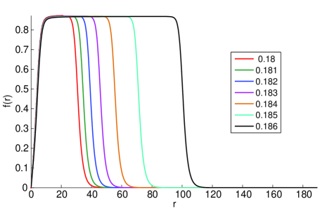
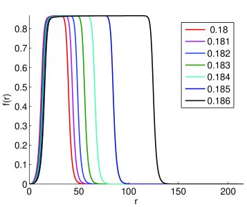
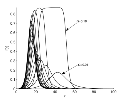
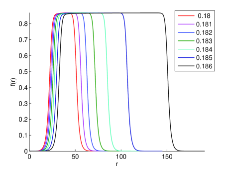
Figure 5: Steady-state vortex radial profiles computed by means of the Gauss-Newton routine for $m=1$ (top left), $m=2$ (top right), and $m=3$ (the bottom row of panels) for the indicated values of $\Omega$. In all cases, the variational ansatz was used as the input (not shown here) with the value of $\Omega^{\ast}$ computed using high-precision arithmetic (see text for details). The radial direction was discretized with a grid spacing of $\Delta r=0.5$. The stopping tolerance of $10^{-7}$ was used in the Gauss-Newton routine. As $\Omega$ approaches the limit value, $3/16$, the profiles flatten out due to the increase of the vortex’ radius.

III Numerically Exact Steady-State Vortex Profiles and Comparison to the Variational approximation

To find numerical solutions to Eq. (4), we used a modified Gauss-Newton optimization routine, with a tolerance $10^{-7}$ NLSxMI . In Fig. 5, some numerically found radial profiles are displayed for charges $m=1$, $m=2$, and $m=3$ and $\Omega>0.18$, including $\Omega$ as close to $\Omega_{\mbox{\scriptsize max}}^{\mbox{\scriptsize 2D}}=\allowbreak 0.187\,5$ as $\Omega=0.186$. To our knowledge, the profiles above $\Omega=0.181$ have not been shown in any previous study. It is seen that the profiles flatten out as $\Omega$ grows, pushing the profile farther from $r=0$. At the same time, the ring of the vortex becomes wider without a change in its height. It is worth mentioning that, due to the high sensitivity of the numerics mentioned in the previous sections, computing profiles past $\Omega=0.18$ is a daunting task requiring high-precision arithmetic. Implementing high-precision arithmetics in a Gauss-Newton optimization routine (or any fixed-point iteration method) would be quite involved and very time consuming. Nonetheless, we have found that, using high-precision arithmetics (up to $300$ decimal places for frequencies as close to $\allowbreak 0.187\,5$ as $0.187$) in the calculation of $\Omega^{\ast}$ in the variational equation (15) yields approximate analytical solutions that the Gauss-Newton subroutine is able to process into numerically accurate solutions for values of $\Omega$ very close to $\Omega_{\mbox{\scriptsize max}}^{\mbox{\scriptsize 2D}}=0.1875$, as shown in Fig. 5. The results clearly demonstrate the usefulness of the VA: without using this approximation for generating the initial profiles to be fed into the numerical solver, a prohibitively complex high-precision fixed-point algorithm would be needed to obtain meaningful profiles past $\Omega=0.18$.

The accuracy of the variational ansatz per se can be tested by comparing it to the numerical solutions computed by means of the Gauss-Newton routine. In Fig. 6 we compare the VA prediction for the vortex-ring’s radius, $r_{c}$, to the numerically found values for $m=5$. We observe that the radii provided by both methods are virtually identical, allowing one to use the VA-predicted radius in applications, that may be useful in experimental situations.

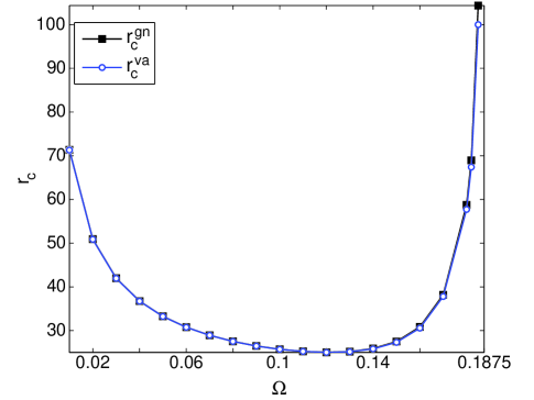
Figure 6: The vortex-ring radius $r_{c}$ versus $\Omega$ as predicted by the variational approximation ($r_{c}^{\mbox{\scriptsize va}}$, white circles), and produced by the Gauss-Newton profile ($r_{c}^{\mbox{\scriptsize gn}}$, black squares) for $m=5$. The numerical radius was computed as the radial center of mass of the vortex ring.

To get an even better idea of how close the variational approach is to the Gauss-Newton profile overall, in Fig. 7 we compare the relative sum of squared deviations of the variational profiles from their the numerically found counterparts, for different values of $m$ and different values of $\Omega$. We also plot a series of profiles produced by the VA and by the Gauss-Newton method for $\Omega=0.15$. We observe that, as $m$ increases, the mismatch between the variational and numerical profiles decreases. This is understandable, as we have neglected the $1/r_{c}$ term in the Laplacian, while formulating the variational ansatz. Therefore, since vortices with smaller $m$ have smaller inner radii, the discrepancy between the variational ansatz and the numerically exact solution are expected for lower values of $m$. The total discrepancy is observed to be quite low overall, showing that the variational profile provides for a very accurate rendition of the true solution, especially for larger values of $m$. Since our VA provides an accurate radial profile of the vortex solitons, we can use it to derive fully analytic azimuthal modulational stability predictions, which is done below.

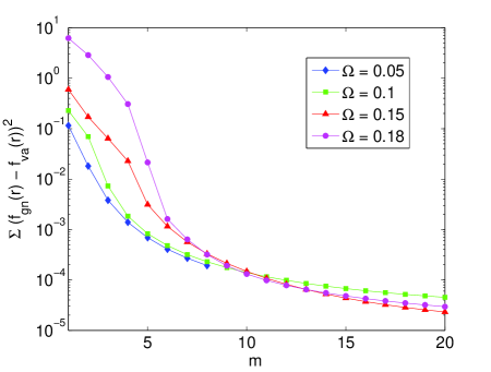
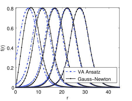
Figure 7: Top: The sum of squared errors between the variationally predicted and numerically found radial profiles of the vortex soliton. Bottom: Examples of the variational (dashed) and numerical (solid) profiles for $\Omega=0.15$. Shown from left to right are the profiles for $m=1,...,5$. It is seen that the error decreases as $m$ increases. The series of error values for $\Omega=0.05$ and $0.1$ terminate at $m=8$ because at that point the variational profiles are already within the prescribed tolerance of $10^{-6}$ of the Gauss-Newton routine.

IV The Azimuthal Modulational Stability: Analytical Results

With the profiles of the steady-state vortices available, we proceed to the study of their azimuthal modulational stability. To this end, we apply the methodology utilized in previous works, dealing with circular gap solitons in the model of the circular Bragg grating Koby , and in the cubic NLS equation NLSxMI : we will derive an azimuthal equation of motion by assuming a frozen radial profile, and then perform a perturbation analysis to analyze the stability of azimuthal perturbation modes.

In Ref. NLSxMI , numerically computed eigenmodes of perturbations around the solitary vortices featured a slight coupling in the radial and azimuthal directions, hence assuming the compete separability of the radial and azimuthal directions for the evolution of the perturbations may lead to discrepancies between the predictions for the stability and numerical results. Nonetheless, the coupling between the radial and azimuthal directions is attenuated with the increase of $m$, hence, the predictions made under the assumption of the separability should be more accurate for higher values of $m$. The trend to the improvement in the accuracy of the analytical approximation with the increase of $m$ was observed in the numerical results presented in Sec. III.

IV.1 The Azimuthal Equation of Motion

To derive the azimuthal equation of motion, we first insert the separable ansatz (2) into the Lagrangian density (8) to obtain

$$\mathcal{L} = \frac{i}{2}f^{2}(r)\,(AA_{t}^{\ast}-A^{\ast}A_{t})+\left(\frac{df}{dr}\right)^{2}\left|A\right|^{2}+$$

$$\frac{1}{r^{2}}f^{2}(r)\left|A_{\theta}\right|^{2}-\frac{1}{2}f^{4}(r)\,\,|A|^{4}+\frac{1}{3}f^{6}(r)\,\,|A|^{6}.$$

Using our steady-state radial profiles, we can perform the integration of the Lagrangian density over $dr$, thus arriving at an effectively one-dimensional (in the direction of $\theta$) Lagrangian that may be used to derive the equation of motion for $A(\theta,t)$:

$$L_{\mbox{\scriptsize 1D}}=\int_{0}^{2\pi}\!\mathcal{L}_{\mbox{\scriptsize 1D}}\,d\theta,$$ (19)

$$\mathcal{L}_{\mbox{\scriptsize 1D}} \equiv \frac{i}{2}C_{1}(AA_{t}^{\ast}-A^{\ast}A_{t})+C_{2}|A|^{2}$$

$$+C_{3}|A_{\theta}|^{2}-\frac{s_{1}}{2}C_{4}|A|^{4}-\frac{s_{2}}{3}C_{5}|A|^{6},$$

and $C_{j}$, $j=1,...,5$, are the radial integrals defined as per Eq. (11). Evaluating the variational derivative of the action functional VA , and applying a linear transformation,

$$A\rightarrow A\,\exp(-iC_{2}t/C_{1}),~{}dt\rightarrow C_{3}t/C_{1},$$ (21)

yields the following evolution equation for $A(\theta,t)$:

$$iA_{t}=-A_{\theta\theta}-\left(C_{4}/C_{3}\right)|A|^{2}A+\left(C_{5}/C_{3}\right)|A|^{4}A.$$ (22)

This equation provides a description of how the radially-frozen, azimuthally time-dependent solution will evolve in the CQNLS model.

IV.2 The Stability Analysis

To study the azimuthal modulational stability of vortex-soliton solutions to the CQNLS equation, we performed a perturbation analysis in the framework of the azimuthal equation of motion (22), with the objective to compute the growth rates of small perturbations. We begin with an azimuthal “plane-wave” solution perturbed by a complex time-dependent perturbation:

$$A(\theta,t)=\left[1+u(\theta,t)+iv(\theta,t)\right]\,e^{i(m\theta+\Omega^{{}^{\prime}}t)},$$ (23)

with $|u|,|v|\ll 1$. Inserting this into Eq. (22), performing the linearization with respect to the perturbations, and separating the result into real and imaginary parts, we obtain a system of coupled equations (a time shift was made here, $t\rightarrow t+\,\theta/\left(2m\right)$):

$$\begin{array}[]{ll}u_{t}=-v_{\theta\theta},&\\[8.61108pt] v_{t}=u_{\theta\theta}+\left(\dfrac{2C_{4}-4C_{5}}{C_{3}}\right)\,u.&\end{array}$$ (24)

In order to study the azimuthal modulational stability of the solitary vortices, we expand $u$ and $v$ into Fourier series over azimuthal harmonics with integer wavenumbers $K$:

$$\hat{u}(K,t) = \int_{0}^{2\pi}\!u(\theta,t)\,e^{iK\theta}\,d\theta,$$

$$\hat{v}(K,t) = \int_{0}^{2\pi}\!v(\theta,t)\,e^{iK\theta}\,d\theta.$$ (25)

Applying these transforms to Eq. (24) yields two coupled equations for the amplitudes of $u$ and $v$ of each mode. In a matrix form, the equations are

$$\frac{d}{dt}\left[\begin{array}[]{c}\hat{u}\\[15.0694pt] \hat{v}\end{array}\right]=\left[\begin{array}[]{cc}0&K^{2}\\[8.61108pt] \left(\dfrac{2C_{4}-4C_{5}}{C_{3}}-K^{2}\right)&0\end{array}\right]\!\left[\begin{array}[]{c}\hat{u}\\[15.0694pt] \hat{v}\end{array}\right].$$ (26)

The growth rates for each azimuthal wavenumber $K$ are simply eigenvalues of Eq. (26). Taking into account the underlying rescaling (21), they are:

$$\lambda_{1,2}=\pm\frac{C_{3}}{C_{1}}\sqrt{K^{2}\left(K_{\mbox{\scriptsize crit}}^{2}-K^{2}\right)},$$ (27)

where $K_{\mbox{\scriptsize crit}}$ is the critical value of $K$, above which all the modes are stable:

$$K_{\mbox{\scriptsize crit}}\equiv\sqrt{\dfrac{2\left(C_{4}-2C_{5}\right)}{C_{3}}}.$$ (28)

For the modulationally unstable vortices, it is useful to know the maximum growth rate and the mode that exhibits it. This is because, in an experiment, even an unstable vortex may be practically “stable enough” if the maximum perturbation growth rate is small enough. This information can be extracted from expression (27) by equating its derivative to zero and solving for $K$, which reveals the fastest growing perturbation mode (and subsequently, the prediction of the number of fragments that the unstable vortices will break up into):

$$K_{\mbox{\scriptsize max}}=\sqrt{\frac{C_{4}-2C_{5}}{C_{3}}}=\frac{1}{\sqrt{2}}K_{\mbox{\scriptsize crit}}.$$ (29)

We can then insert this value into Eq. (28), which yields the maximum growth rate,

$$\lambda_{\mbox{\scriptsize max}}=\frac{C_{4}-2C_{5}}{C_{1}}=\frac{C_{3}}{2C_{1}}K_{\mbox{\scriptsize crit}}^{2}.$$ (30)

In fact, because $K$ must be integer, the actual fastest growing eigenmode may correspond to the integer $K$ closest to value (29). Accordingly, the actual largest growth rate may be somewhat smaller than the one given by Eq. (30).

For the vortex to be azimuthally stable against all modes, one needs either $K_{\mbox{\scriptsize crit}}<1$ (then, there is no integer value $K<K_{\mbox{\scriptsize crit}}$) or $K_{\mbox{\scriptsize crit}}$ being purely imaginary. According to Eq. (28), these two stability criteria amount to the following inequalities:

$$\mathrm{imaginary}~{}~{}K_{\mbox{\scriptsize crit}}:~{}~{}C_{4}-2C_{5}<0;$$ (31)

$$\left|K_{\mbox{\scriptsize crit}}\right|<1:~{}~{}C_{4}-2C_{5}-C_{3}/2<0.$$ (32)

Since $C_{3}$ is positive, the former condition is stricter than the latter one. Although the latter condition is sufficient for the azimuthal stability, we also keep the former one (according to the above derivation, it is relevant to the infinite line) because it leads to an estimation for the critical frequency which is independent of charge $m$ (see below).

For our predictions, we compute the $C_{i}$ constants using numerical integrals of the numerically exact radial profiles. However, since the variational analytic profiles are so close to the numerically exact profiles, one can use expressions (12) to find approximate analytic values of Eqs. (31) and (32), which then yield critical values $\Omega_{\mbox{\scriptsize st}}(m)$ of $\Omega$, above which all the vortex solitons are azimuthally stable for charge $m$. These values can then be compared to those computed by the numerically exact profiles.

IV.3 Analytical Stability Predictions Using the Variational Profile

As we showed in Sec. III, the variational ansatz yields a useful approximation to the true radial profiles. Therefore, the VA can be employed to calculate the constants in Eq. (12), and thereby derive analytical predictions for the azimuthal modulational stability. In Sec. IV.2 it was demonstrated that, for studying the stability of the vortices, only the values of $K_{\mbox{\scriptsize crit}}$ and $C_{3}/C_{1}$ are required,

$$K_{\mbox{\scriptsize crit}}^{\mbox{\scriptsize va}}=m\sqrt{\frac{6\Omega^{\ast}-\left(15/8\right)+5\sqrt{3\Omega^{\ast}}/\left(4T\right)}{\Omega^{\ast}-G(\Omega^{\ast})}},$$ (33)

$$\left(\frac{C_{3}}{C_{1}}\right)_{\mbox{\scriptsize va}}\!=\frac{\Omega^{\ast}-G(\Omega^{\ast})}{m^{2}},$$ (34)

since the other coefficients can be expressed in terms of these two (here, as before, $\Omega=G(\Omega^{\ast})$).

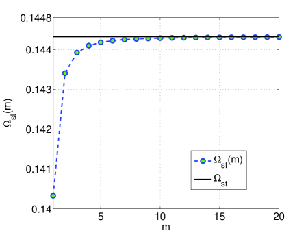
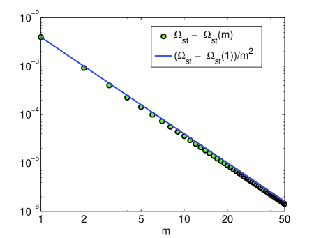
Figure 8: (Color online) Top: The critical value of frequency $\Omega_{\mbox{\scriptsize st}}^{\mbox{\scriptsize va}}(m)$ versus topological charge $m$, according to the prediction of the variational approach. Bottom: The rate of the convergence between $\Omega_{\mbox{\scriptsize st}}^{\mbox{\scriptsize va}}(m)$ and $\Omega_{\mbox{\scriptsize st}}^{\mbox{\scriptsize va}}$ at increasing $m$. The plotted curve, $\mathrm{const}\times m^{-2}$, which starts from our $m=1$ computed value, demonstrates that the convergence rate is proportional to $1/m^{2}$.

The VA can predict the critical value of $\Omega^{\ast}$ above which the vortices are modulationally stable. Inserting the constants defined in Eq. (12) into the stability criteria (31) and (32), we arrive at the following expressions which determine the critical frequency:

$$K_{\mbox{\scriptsize crit}}=0:~{}~{}6\Omega^{\ast}-\frac{15}{8}+\frac{5\sqrt{3\Omega^{\ast}}}{4T}=0;$$ (35)

$$K_{\mbox{\scriptsize crit}}=1:~{}~{}\sqrt{\frac{6\Omega^{\ast}-15/8+5\sqrt{3\Omega^{\ast}}/\left(4T\right)}{\Omega^{\ast}-G(\Omega^{\ast})}}-\frac{1}{m}=0,$$ (36)

where $T$ is defined as per Eq. (13). We see that, at $m\rightarrow\infty$, these two criteria tend to coincide. At finite $m$, Eqs. (35) and (36) give different critical values of $\Omega^{\ast}$, and hence of $\Omega$ too —one which depends on charge $m$, and the other one, independent of $m$, which represents an upper bound on $K_{\mbox{\scriptsize crit}}$ for all values of $m$. We denote the charge-dependent critical value as $\Omega_{\mbox{\scriptsize st}}(m)$, and the charge-independent one as $\Omega_{\mbox{\scriptsize st}}$.

Solving Eq. (35) for $\Omega^{\ast}$ by means of a root finder and inserting the result into Eq. (15) yields

$$\Omega_{\mbox{\scriptsize st}}^{\mbox{\scriptsize va}}=0.144320424.$$ (37)

Since this value is smaller than $\Omega_{\mbox{\scriptsize max}}^{\mbox{\scriptsize 2D}}=3/16$, this result predicts that azimuthally stable vortices exist for all values of $m$, at $\Omega>\Omega_{\mbox{\scriptsize st}}^{\mbox{\scriptsize va}}$. We also solved Eq. (36) for $\Omega$ at various values of $m$. The results are displayed in Fig. 8. It is seen that the critical frequency $\Omega_{\mbox{\scriptsize st}}^{\mbox{\scriptsize va}}(m)$ increases with the increase of $m$ and eventually converges to $\Omega_{\mbox{\scriptsize st}}^{\mbox{\scriptsize va}}$. Thus, the stability window in $\Omega$ is larger for lower charges. In Ref. AMIxCQNLSxNEW , it was also concluded that azimuthally stable vortices exist for all $m$, and that lower charges indeed have a larger stability window. However, according to Ref. AMIxCQNLSxNEW , $\Omega_{\mbox{\scriptsize st}}=\Omega_{\mbox{\scriptsize max}}^{\mbox{\scriptsize 2D}}$, i.e., the stability window shrinks towards $0$ as $m\rightarrow\infty$. The estimate obtained in that work shows that the window shrinks as $1/m^{2}$. This conclusion precludes experimental creation of higher-order stable vortices, as the respective stability interval would be too small, and the radius of the vortex too large.

According to the VA predictions, $\Omega_{\mbox{\scriptsize st}}$ does increase with $m$ (and, as shown in Fig. 8, the difference $\Omega_{\mbox{\scriptsize st}}-\Omega_{\mbox{\scriptsize st}}(m)$ decays proportionally to $1/m^{2},$ which resembles the prediction of Ref. AMIxCQNLSxNEW ). On the other hand, since the variationally predicted value of $\Omega_{\mbox{\scriptsize st}}$ is smaller than $3/16$, there remains a stability window at all $m$, which does not vanish at $m\rightarrow\infty$.

As shown in Table 2, the variational predictions are very close to those using the numerically-exact profiles. We then note that the numerical results reported in Ref. AMIxCQNLSxNEW are more accurate than our predictions, the stability window indeed shrinking to zero at high values of $m$.

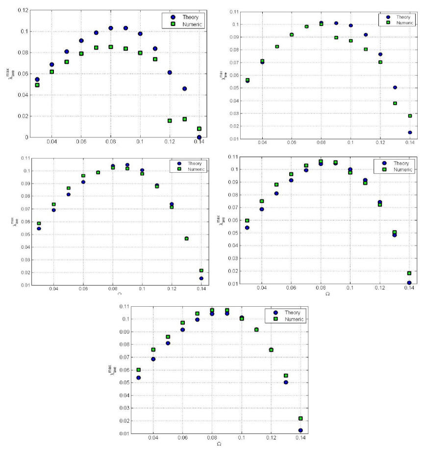
Figure 9: (Color online) Numerical predictions and numerical results for the growth rates of the fastest growing unstable perturbation mode around vortex solitons with charges $m=1,...,5$ (left to right, top to bottom). In the interval of $\Omega\in\left[0.03,0.14\right]$, with the step of $\Delta\Omega=0.01$, the growth-rate predictions (shown by circles) were obtained by computing the integrals in the underlying Lagrangian, using the numerically exact profiles obtained through the Gauss-Newton optimization. We then ran full simulations of the vortex and recorded the average instability growth rate (shown by squares). The radial, angular, and temporal variables were discretized with steps $\Delta r=1$, $\Delta\theta=(2\pi)/(20\,\mbox{max}[m,K_{\mbox{\scriptsize max}},2])$, and $\Delta t=0.001$, respectively. Overall, the predictions match the numerical results very well.

V Azimuthal Modulational Stability: Numerical Results

In this section we report the numerical predictions and full simulation results for the azimuthal modulational (in)stability of the vortices. For the 2D simulations, we used a finite-difference scheme with a central difference in space and fourth-order Runge-Kutta in time NUMODE . We used both polar-coordinate and Cartesian grids. The polar grid makes computing the growth of individual perturbation modes easier, therefore we used it to test our predictions for azimuthally unstable vortices. However, the polar grid forces one to use smaller time steps in the finite-difference scheme than is needed for the equivalent Cartesian grid. Therefore, for testing the critical frequency $\Omega_{\mbox{\scriptsize st}}(m)$, which requires running multiple long-time simulations, we use the Cartesian grid. We used second-order differencing for the polar-coordinate simulations, and (due to the long simulation time needed) a fourth-order differencing for the Cartesian simulations.

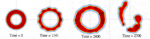
Figure 10: (Color online) Examples of the evolution of a vortex with charge $m=4$ and $\Omega=0.18$, perturbed by a random perturbation of size $\epsilon=0.05$. Pictured is the squared absolute value of the wave function. We have set $\Delta r=2$, $r_{\mbox{\scriptsize max}}=120$ and $\Delta t=0.6$. The initial vortex shape becomes deformed and then breaks up irregularly.

V.1 Unstable Vortices

In Fig. 9 we show the results for the (in)stability of vortices with charges $m=1,...,5$ and $\Omega\in[0.03,0.14]$. In general, we see a good agreement between the numerically measured growth rates and the predictions for $m>2$; however, for values of $\Omega$ which get closer to $3/16$, the accuracy of the predictions becomes low in each case, implying that our predictions for $\Omega_{\mbox{\scriptsize st}}(m)$ are not precise. To further test this, we ran long-time simulations of randomly perturbed vortices.

For $m=1,2,3$, we were easily able to identify the transition from unstable to stable vortices, but for $m>3$ we found it very difficult to detect a stable solution, because of a snake-like instability which breaks the vortex into asymmetric irregular fragments. An example of this is shown in Fig. 10. Obviously, this snake-like instability is not captured by our study of the azimuthal modulational instability. It is very plausible that it accounts for the discrepancy between the analytic and numerical growth rates observed in Fig. 9.

V.2 Stable Vortices

To identify the values of $\Omega_{\mbox{\scriptsize st}}(m)$ corresponding to the stability border, we simulated the evolution of vortices with $\Omega$ taken near the predicted values of $\Omega_{\mbox{\scriptsize st}}(m)$, perturbed by a small uniformly distributed random noise in the azimuthal direction. Our aim was to find a value $\Omega_{1}$ of $\Omega$ that results in an unstable vortex soliton (and to observe the actual breakup), and then show that the vortex solution for $\Omega_{2}=\Omega_{1}+0.001$ is stable, by simulating its evolution for an extremely long time, compared to the time necessary to reveal the full breakup in the former case. We did this for various charges $m$. In Fig. 11, we show the initial and final states produced by this analysis for $m=1$.

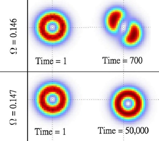
Figure 11: (Color online) An example of the numerical identification of the stability border, $\Omega_{\mbox{\scriptsize st}}(m)$, for $m=1$. In this case, the evolution of the vortex with $\Omega_{1}=0.146$ (top left) was simulated with a random-noise perturbation in the azimuthal direction, until it broke up into fragments due to the azimuthal instability (top right). We then carried out long simulations of the evolution of a vortex with $\Omega_{2}=\Omega_{1}+0.001=0.147$ (bottom left), to make it sure that the vortex is stable —in this example, up to $t=50,000$ (bottom right). The drift of the position of the vortical pivot is due to the momentum imparted to it by the random perturbations. We thus conclude that $\Omega_{\mbox{\scriptsize st}}(m=1)\in\left[0.146,0.147\right]$. In this example, we set the grid spacing to be $\Delta x=\Delta y=1$, time step to $\Delta t=0.2$, and the perturbation amplitude to $\epsilon=0.05$.

Since the snaking effect hinders our ability to simulate the evolution of the vortices for extended time periods at $m>3$, we were not able to make precise stability predictions in this case. However, as this effect is dynamically distinct from the azimuthal breakup, we can still give an approximate estimate of the critical frequency for higher charges.

In Table 2 we display the predictions of $\Omega_{\mbox{\scriptsize st}}(m)$ and their numerically found counterparts for $m=1,...,5$. The column labeled “semi-numerical” are the predictions made using the numerically exact radial profiles, while the column labeled “VA” gives the predictions made using the variationally derived profiles. For comparison, in the same Table we also display findings reported in earlier works. We see that most of the predictions for $m=1$ are close to the numerical result. For $m>1$, the results reported in Ref. AMIxCQNLSxNEW are most accurate ones.

$m$	NUM	semi-NUM	VA	Ref. AMIxCQNLSxNEW	Ref. AMIxCQNLSxLONG	Ref. AMIxCQNLSxOLD
1	0.147	0.1399	0.1403	0.1487	0.16	0.145
2	0.162	0.1433	0.1434	0.1619	0.17	NC
3	0.171	0.1437	0.1439	0.1700	NC	NC
4	(0.178)	0.1437	0.1441	0.1769	NC	NC
5	(0.18)	0.1437	0.1442	0.1806	NC	NC

Table 2: Comparison of the predictions and numerical results for the stability border, $\Omega_{\mbox{\scriptsize st}}(m)$. The columns labeled “semi-NUM” and “VA” represent the predictions utilizing the numerically exact and the variationally derived radial profiles respectively. The column labeled “NUM” are the results obtained from the full 2D simulations. Numerical findings in parentheses are those that were hard to fix due to the emergence of the snake-like instability (not comprised by our stability analysis), and may therefore be less accurate than the others. We also show predictions reported in earlier works. When no value has been computed or reported, we label the entry as “NC”. The predictions made in Ref. AMIxCQNLSxNEW are the most accurate ones, in comparison to our simulations.

It is observed that the semi-numerical and variational results are very close, the latter ones being, in fact, slightly more accurate in comparison with the numerical findings. This implies that the discrepancies in the variationally derived predictions are not due to any inherent deficiency in the VA. Rather, the discrepancies of both sets of predictions are likely due to the approximation of the vortex soliton as a separable entity composed of radial and azimuthal parts (as discussed in Sec. IV).

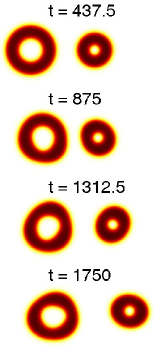
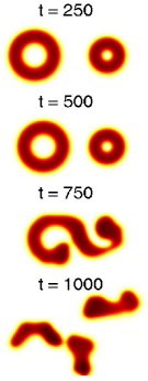
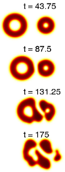
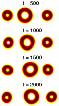
Figure 12: (Color online) Collisions between stable vortices, all with frequency $\Omega=0.17$. First column: an elastic collision between a moving vortex of charge $m=2$, with a slow initial velocity of $0.03$, and a stationary vortex of charge $m=1$. The vortices have no relative phase difference between them, which corresponds to their colliding sides being out-of-phase, hence the interaction is repulsive. Accordingly, the vortices undergo an elastic collision. Second column: the same as in the first column, but with a $\pi$ phase difference between the colliding vortices, which implies that their colliding sides are in phase. This, in turn, gives rise to a mutual attraction, which causes the vortices to merge and eventually break up into fragments. Third column: same as in the first column, but for a larger collisional velocity of $0.3$. The mutual repulsion between the in-phase vortices is not enough to counterbalance the high collisional momentum, and the vortices merge and break up into fragments. Fourth column: a charge $m=1$ vortex with velocity $0.03$ undergoing an elastic collision with an $m=2$ vortex, in the case of a $\pi$ phase difference between them, which in turn collides with another $\pi$-phase-shifted vortex of charge $m=1$. This phase arrangement corresponds to vortices colliding with adjacent sides that are mutually $\pi$-out-of-phase, and thus repel each other. These results attest to the robustness of the vortices.

VI Collisions and Scattering of Stable Vortices

In this section we study collisions and scattering of stable vortices in the CQNLS. In Ref. AMIxCQNLSxOLD , such collisions of vortices of unit charge were considered in a brief form. It was shown that both elastic and destructive collisions could be observed depending on the phase difference, $\Delta\phi$, between the colliding vortices, as well as on their relative velocity. Here we expand this study in three directions: i) we include vortices of charge $m=2$; ii) we consider the critical velocity for elastic collisions as a function of $\Delta\phi$; iii) we study the scattering of vortices colliding at various values of impact parameters, by measuring the scattering angles and speeds.

Summarizing results of numerous simulations, we have found that, at sufficiently small collisional velocities, the elastic or destructive character of the collision is solely determined by the phase difference at the point of contact. This fact seems to be independent of the charge of the vortices involved in the collision. In Fig. 12 we display four different cases that illustrate the main features of head-on collisions between vortices with different charges. In the first two columns of Fig. 12 we show the collision of vortices carrying charges $m=2$ and $m=1$, with $\Delta\phi=0$ and $\Delta\phi=\pi$, respectively. It can be seen that, since the vortex with $m=2$ has opposite phase on the collision side, with respect to the vortex with $m=1$, the interaction is repulsive since it locally emulates the interaction of two out-of-phase fundamental bright solitons interaction ; adhikari03 . Therefore, if the velocity is small enough, the mutual repulsion determines the result of the collision. On the other hand, when the vortex with charge $m=2$ is phase-shifted by $\pi$ (or similarly, if the charge $m=2$ vortex were to be placed on the opposite side of the charge $m=1$ vortex), the adjacent sides of the colliding vortices are in phase. Therefore, the interaction is similar to that between two in-phase bright solitons, which is attractive interaction ; adhikari03 . This results in the merger of the two vortices and their eventual breakup into fragments.

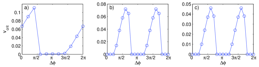
Figure 13: (Color online) Critical velocity $v_{\mathrm{crit}}$ for elastic collisions between two vortices as a function of their phase difference $\Delta\phi$. The vortex charges of the colliding vortices correspond to: (a) $(m_{1},m_{2})=(1,1)$, (b) $(m_{1},m_{2})=(1,2)$, and (c) $(m_{1},m_{2})=(2,2)$. All vortices are taken with intrinsic frequency $\Omega=0.17$.

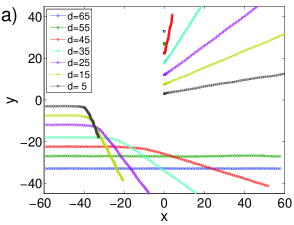
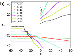
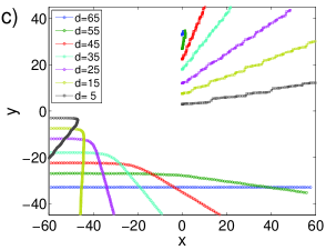
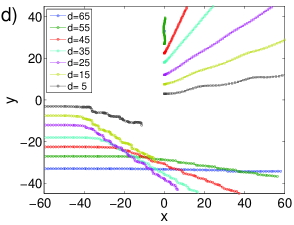
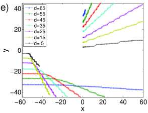
Figure 14: (Color online) Scattering between an incoming vortex with charge $m_{1}$ and velocity $v_{1}^{\mathrm{ini}}$, and a quiescent vortex of charge $m_{2}$. The trajectory for the incoming (stationary) vortex is depicted by small circles (squares). All panels depict different trajectories for different values of impact parameter $d$, as indicated [$d=5,15,25,...,65$ from top to bottom (bottom to top) for the incoming (stationary) vortex]. Panels (a) and (b) correspond, respectively, to two unitary-charge vortices ($m_{1}=m_{2}=1$), with $\Delta\phi=0$ and collision velocities $v_{1}^{\mathrm{ini}}=0.03$ and $v_{1}^{\mathrm{ini}}=0.06$. Panels (c) and (d) correspond, respectively, to a $m_{1}=1$ vortex scattered by a $m_{2}=2$ one and vice versa, for the collision velocity $v_{1}^{\mathrm{ini}}=0.03$ and $\Delta\phi=\pi/2$. Panel (e) corresponds to a $m_{1}=2$ vortex scattered by a $m_{2}=2$ one, for $v_{1}^{\mathrm{ini}}=0.02$ and $\Delta\phi=\pi/2$. All vortices have intrinsic frequency $\Omega=0.17$.

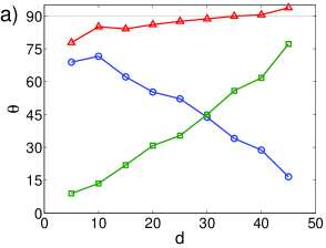
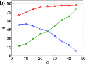
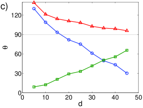
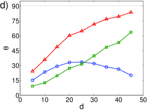
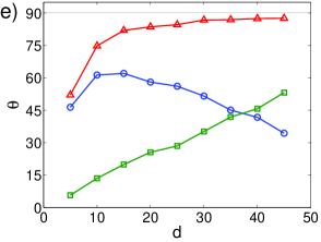
Figure 15: (Color online) Scattering angles for the collision of two vortices corresponding to the panels depicted in Fig. 14. Depicted by (blue) circles is the negative of the scattering angle $-\theta_{1}$ of the incoming vortex, while (green) squares stand for the scattering angle $\theta_{2}$ of the initially quiescent vortex. Triangles (in red) display the difference between these two angles, $\theta_{2}-\theta_{1}$. All angles are given in degrees.

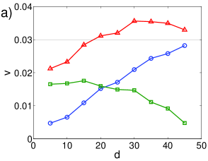
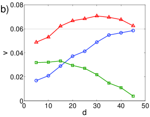
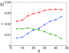
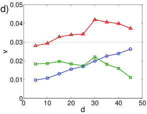
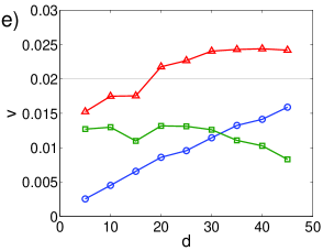
Figure 16: (Color online) Final (post-collision) velocities for the scattering of two vortices corresponding to the panels depicted in Fig. 14. Depicted in (blue) circles and (green) squares are, respectively, the final velocities, $v_{1}$ and $v_{2}$, of the initially moving and quiescent vortices. (Red) triangles depict the sum of these two velocities, $v_{1}+v_{2}$. The thin horizontal black line designates the initial velocity of the moving vortex.

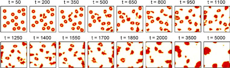
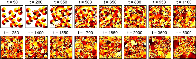
Figure 17: Interaction of a random gas of vortices of charge $m=1$ in a periodic box. The initial separation between any two neighboring vortices exceeds twice the width of a single vortex. The initial phases are set randomly. The first two rows depict the evolution of the field intensity at the times indicated, while the bottom two rows depict the respective phase of the field. Note the coarsening effect due to vortex merger and destruction.

Clearly, even when the repulsive force acts between vortices, but the collision velocity is sufficiently large, the vortices have enough momentum for causing them to merge and eventually break up as well. This case is depicted in the third column of Fig. 12.

Slowly moving vortices with opposite phases at the point of contact are quite robust against the collisions, as illustrated in the fourth column of Fig. 12. In this panel we depict a “billiard”-type example, in which one vortex collides with another, which in turn collides with a third one. All collisions in this case are elastic because the relative phases have been chosen such that the colliding sides are always out-of-phase, providing for the necessary repulsion. It is worthy to note that, although these collisions at low velocities seem to be elastic, the stable vortices clearly have internal breathing modes, that are excited during the collisions. Therefore, a small fraction of the collisional energy is transferred to these internal modes, preventing the collisions from being completely elastic. A more in-depth analysis of the excitation of these internal modes and of the degree of the inelasticity of the collisions fall outside of the scope of the present work. Nonetheless, in order to quantify the degree of the elasticity of the collisions, we have measured the critical velocity $v_{\mathrm{crit}}$ for the vortices to elastically bounce off each other: at $v<v_{\mathrm{crit}}$ the vortices bounce elastically, while at $v>v_{\mathrm{crit}}$ they merge and, most often, get destroyed. The crucial parameter that controls $v_{\mathrm{crit}}$, for a particular combination of the charges of colliding vortices, is their phase difference ${\Delta}$$\phi$. Different values of $\Delta\phi$ allow to have different relative phases at the colliding sides (as discussed above), and thus (partially) repel or attract. This effect is illustrated by Fig. 13, where we depict $v_{\mathrm{crit}}$ versus ${\Delta}$$\phi$ for vortex pairs with charges (a) $(m_{1},m_{2})=(1,1)$, (b) $(m_{1},m_{2})=(1,2)$, and (c) $(m_{1},m_{2})=(2,2)$. From panel (a) it is clear that, for charges $m_{1}=m_{2}=1$, the most “stable” (in terms of observing elastic collisions at larger collisional velocities) collision occurs around ${\Delta\phi=0}$. This corresponds exactly to the most stable case mentioned above, when the collisional sides are out of phase. In panel (b) we depict $v_{\mathrm{crit}}$ for $(m_{1},m_{2})=(1,2)$. It is seen in this panel that $v_{\mathrm{crit}}$ is $\pi$-periodic, as a function of $\Delta\phi$, due to the angular symmetry of the $m_{2}=2$ vortex. For this vortex-charge combination, the most stable collision occurs around ${\Delta}$$\phi=\pi/2$ (or, due to the symmetry, ${\Delta}$$\phi=3\pi/2$), which again corresponds to the adjacent out-of-phase sides. Finally, in panel (c) we present the results for two vortices with $m_{1}=m_{2}=2$. The behavior is very similar to that in panel (b): the same periodicity, shape and value of the optimal phase difference. However, since the vortices with $m=2$ vortices are less stable than those with $m=1$, the critical velocity $v_{\mathrm{crit}}$ is lower for the $(m_{1},m_{2})=(2,2)$ charge combination than for the case of $(m_{1},m_{2})=(1,2)$.

In order to fully characterize the collisions between vortices with different charges, we studied the scattering of a vortex of charge $m_{1}$ impinging at velocity $v_{1}^{\mathrm{ini}}$ upon another vortex of charge $m_{2}$ at rest ($v_{2}^{\mathrm{ini}}=0$), with impact parameter $d$. The impact parameter $d$ is defined as the perpendicular distance between the trajectory of the incoming vortex and the initially quiescent one. In Fig. 14 we show several orbits for the two vortices with different impact parameters, vortex-charge combinations, and incoming velocities. It is seen, in all the panels, that all the trajectories are well defined for the chosen parameters, and clearly feature elastic scattering. The key to achieve elastic scattering is to choose, for each charge combination, the optimal phase difference, using Fig. 13 [i.e., $\Delta\phi=0$ for $m_{1}=m_{2}=1$ and ${\Delta}$$\phi=\pi/2$ for $(m_{1},m_{2})=(1,2)$, $(2,1)$, or $(2,2)$], and the initial velocity lower than the corresponding $v_{\mathrm{crit}}$. For example, we chose in panel (a) of Fig. 14 $\Delta\phi=0$ and $v_{2}^{\mathrm{ini}}=0.03<v_{\mathrm{crit}}(\pi=0)=0.067$. In fact, when one uses a velocity closer to the critical one the vortices start experiencing strong deformations of the quadrupole and octupole types when they collide nearly head-on. This effect is clearly visible for the trajectory with $d=5$ (also $d=10$ and $d=20$) in panel (b) of Fig. 14, where $v_{2}^{\mathrm{ini}}=0.06$ is close to the critical value, $v_{\mathrm{crit}}=0.067$, and the trajectory features undulations due to the internal deformation of the vortex. Even larger velocities, i.e., above $v_{\mathrm{crit}}$, lead to elastic scattering for larger values of the impact parameter $d$, and to annihilation of the colliding vortices at smaller $d$ (not shown here). It is interesting to note that, as for hard spheres with different masses, the scattering of vortices can also produce very different scattering angles, depending on the mass combination of the two colliding objects. This effect is made evident by the comparison of the scattering between vortices with $m_{1}=1$ and $m_{2}=2$ in panel (c), and the scattering between $m_{1}=2$ and $m_{2}=1$ in panel (d) (all the other parameters coincide in both panels). When a “lighter” vortex with $m_{1}=1$ collides with the “heavier” one, with $m_{2}=2$, for $d\leq 15$, the former vortex bounces back after the collisions. In the reverse situation, with the “heavier” $m_{2}=2$ vortex impinging upon the “lighter” one with $m_{1}=1$, the “heavier” vortex only loses a portion of its momentum and continues to move in a straighter trajectory, while the “lighter” vortex is pushed away at a larger velocity.

To further characterize the scattering between vortices we analyzed the scattering angle as a function of the impact parameter. In our scattering experiments, we initially define horizontally moving and quiescent vortices. After the collision, the trajectory of the moving vortex is deviated by scattering angle $\theta_{1}$ (in our case negative since we consider the moving vortex placed below the quiescent one), and the initially quiescent vortex is scattered at angle $\theta_{2}$ (in our case, positive). In Fig. 15 we depict the scattering angles corresponding to the scattering experiments displayed in Fig. 14. We depict by (blue) circles the negative of the scattering angle, $-\theta_{1}$, of the incoming vortex, and by (green) squares the scattering angle $\theta_{2}$. In all the cases, we also depict the difference between the scattering angles, $\Delta\theta=\theta_{2}-\theta_{1}$, by (red) triangles. In the case of the elastic collision between two hard spheres of equal masses it is well known that $\Delta\theta=90^{\mathrm{o}}$. Figure 15 reveals that the collisions between vortices with equal charges [$m_{1}=m_{2}=1$ in panels (a) and (b), and $m_{1}=m_{2}=2$ in panel (e)] produce $\Delta\theta$ very close to ${90}^{\mathrm{o}}$ for all values of the impact parameter. In contrast, as it is the case for hard spheres with different masses, our simulations demonstrate that $\Delta\theta>90^{\mathrm{o}}$ for $m_{1}<m_{2}$ [$(m_{1},m_{2})=(1,2)$ in panel (c)], and that $\Delta\theta<90^{\mathrm{o}}$ for $m_{1}>m_{2}$ [$(m_{1},m_{2})=(2,1)$ in panel (d)].

Another measure of the scattering can be given in terms of the initial and final velocities. In Fig. 16, we present the final velocities corresponding to the scattering events shown in Fig. 14. The figure shows, by (blue) circles and (green) squares, the post-collision velocities, $v_{1}$ and $v_{2}$, respectively, of the initially moving and quiescent vortices. We also depict, using (red) triangles, the sum of the final velocities, $v_{1}+v_{2}$, and the thin horizontal black line represents the initial velocity of the moving vortex, $v_{1}^{\mathrm{ini}}$. It can be concluded that $v_{1}+v_{2}<v_{1}^{\mathrm{ini}}$ for relatively small values of the impact parameter, $d$, and $v_{1}+v_{2}>v_{1}^{\mathrm{ini}}$ for larger values of $d$.

The above results suggest that the interactions between vortices may be either elastic or destructive, depending on the parameters. In order to simulate the interplay of these interactions in a multi-vortex gas, we display in Fig. 17 a time series depicting the time evolution of a random vortex gas. The first two rows depict the local intensity plots at the indicated moments of time, while the bottom two rows depict the corresponding field phases. We use a square domain of size $120\times 120$ with periodic boundary conditions, seeding 15 vortices of charge $m=1$ at random positions (such that initially no two vortices were closer than twice the size of a single vortex), and with random phases. As seen from the figure, due to the random phase differences and collision angles, some vortex pairs experience elastic collisions, while others tend to merge and destroy each other. Since the destruction of vortices is an irreversible process, all the vortices get eventually destroyed, leading to a seemingly disordered pattern of interacting intensity patches with an approximately constant phase inside each one (see the correspondence between field patches in the top rows and the phase patches in the bottom rows, at the late stage of the evolution). The dynamics resembles the grain coarsening in typical chaotic spatiotemporal systems, see e.g., review sand .

VII Conclusions

In this work, we have revisited the issues of the existence, stability, and interactions of solitary vortices in the two-dimensional CQNLS (cubic-quintic nonlinear Schrödinger) equation, using both numerical and analytical methods. The latter one is based on the variational approach, that has been shown to be increasingly more accurate as the vortex’ topological charge increases. We have also developed the analysis of the azimuthal modulational (in)stability of vortices, using the approximation originally proposed in other contexts in Refs. Koby and NLSxMI , which postulates the separation between the frozen radial profile of the vortex soliton and free evolution of azimuthal perturbations. This approach leads to an effectively one-dimensional equation for the azimuthal dynamics. Examining the stability of the perturbed annulus within the framework of the latter equation, we were able to predict the stability of the vortices against the breakup. We then ran full 2D simulations to verify the semi-analytical predictions.

For azimuthally unstable vortices, our predictions of the largest growth rate are fairly accurate over a wide range of the vortex’ intrinsic frequency (especially for the higher-order vortices, with topological charge $m>2$). The so developed semi-analytical technique may be useful for other applications. The analytical approach is less accurate in predicting the stability border (intrinsic critical frequency of the vortex) for $m>1$. This discrepancy is due to deviation from the assumption admitting the separation of the perturbed evolution into radial and azimuthal parts, while the VA proper, which was used to predict the radial shape of the stationary vortex solitons turns out to yield accurate results. Comparing our numerical results for the critical frequency with previously published ones, we have concluded that the most accurate findings were reported in Ref. AMIxCQNLSxNEW . We have also found that higher-order vortices may be subject to a snaking radial instability.

The semi-analytical approach developed in this work may be quite useful for other 2D models —at least, for the description of the most stable vortex solitons with lowest values of the topological charge.

We have also investigated, in detail, collisions between stable vortex solitons in the two-dimensional CQNLS equation. The outcome of the collision crucially depends on the phase difference and relative velocity of the vortices. We have produced the results showing the critical velocity for elastic collisions as a function of the relative phase for all combinations of the vortices with $m=1$ and $2$. We also studied the dependence on the scattering angles and post-collision velocities on the impact parameter of the collision.

One relevant direction for the extension of the present analysis is to find accurate conditions for the stabilization of the nearly isotropic vortex solitons by an external spatially periodic (lattice) potential, see Ref. Sakaguchi and references therein. A challenging problem is to extend the semi-analytical considerations to three-dimensional solitons with embedded vorticity, in the model with the same cubic-quintic nonlinearity. In fact, it is not known if such 3D vortex solitons with higher vorticity ($m\geq 2$) may be stable PRL ; Torner .

VIII Acknowledgments

The authors thank Juan Belmonte and Jesús Cuevas for providing useful insights. RCG gratefully acknowledges support from NSF-DMS-0806762. PGK gratefully acknowledges support from NSF-DMS-0349023 (CAREER) and NSF-DMS-0806762, as well as from the Alexander von Humboldt Foundation.

References

- (1) S. K. Adhikari, Mean-field model of interaction between bright vortex solitons in Bose-Einstein condensates, New J. Phys. 5 (2003) 137.1–137.13.
- (2) G. S. Agarwal, S. Dutta Gupta, T-matrix approach to the nonlinear susceptibilities of heterogeneous media, Phys. Rev. A 38 (1988) 5678–5687.
- (3) I. S. Aranson, L. S. Tsimring, Patterns and collective behavior in granular media: Theoretical concepts, Rev. Mod. Phys. 78 (2006) 641–692.
- (4) E. L. Falcão-Filho, C. B. de Araújo, J. J. Rodrigues, Jr, High-order nonlinearities of aqueous colloids containing silver nanoparticles, J. Opt. Soc. Am. B 24 (2007) 2948–2956.
- (5) B. B. Baizakov, B.A. Malomed, M. Salerno, Multidimensional solitons in periodic potentials, Europhys. Lett. 63 (2003) 642–648.
- (6) Juan Belmonte, personal communication.
- (7) J. Scheuer and B. Malomed, Annular gap solitons in Kerr media with circular gratings, Phys. Rev. A 75 (2007) 063805.
- (8) R. M. Caplan, Q. E. Hoq, R. Carretero-González, P. G. Kevrekidis, Azimuthal modulational instability of vortices in the nonlinear Schrödinger equation, Opt. Commun. 282 (2009) 1399–1405.
- (9) S. Cowan, R. H. Enns, S. S. Rangnekar, S. S. Sanghera, Quasi-soliton and other behavior of the nonlinear cubic-quintic Schrödinger equation, Can. J. Phys. 64 (1986) 311–315.
- (10) L. Crasovan, B.A. Malomed, D. Mihalache, Spinning solitons in cubic-quintic nonlinear media, Pramana J. Phys. 57 (2001) 1041–1059.
- (11) A. Desyatnikov, A. Maimistov, B.A. Malomed, Three-dimensional spinning solitons in dispersive media with the cubic-quintic nonlinearity, Phys. Rev. E 61, 3 (2000) 3107–3113.
- (12) K. Dolgaleva, H. Shin, R. W. Boyd, Observation of a microscopic cascaded contribution to the fifth-order nonlinear susceptibility, Phys. Rev. Lett. 103 (2009) 113902.1–113902.4.
- (13) A. L. Fetter, Rev. Mod. Phys. 81, 647 (2009).
- (14) W. J. Firth, D. V. Skryabin, Optical solitons carrying orbital angular momentum, Phys. Rev. Lett. 79 (1997) 2450–2453.
- (15) R. A. Ganeev, M. Baba, M. Morita, A. I. Ryasnyansky, M. Suzuki, M. Turu, H. Kuroda, Fifth-order optical nonlinearity of pseudoisocyanine solution at 529 nm, J. Opt. A: Pure Appl. Opt. 6 (2004) 282–287.
- (16) G. H. Golub, J. M. Ortega, Scientific computing and differential equations an introduction to numerical methods, Academic Press, San Diego, California, 2 edition, 1992.
- (17) B. Gu, Y. Wang, W. Ji, J. Wang, Observation of a fifth-order optical nonlinearity in Bi0.9La0.1Fe0.98Mg0.02O3 ferroelectric thin films, Appl. Phys. Lett. 95 (2009) 041114.1–041114.3.
- (18) G. Herring, L. D. Carr, R. Carretero-González, P. G. Kevrekidis, D. J. Frantzeskakis. Radially symmetric nonlinear states of harmonically trapped Bose-Einstein condensates, Phys. Rev. A 77 (2008) 023625.1–023625.11.
- (19) Yu. S. Kivshar, J. Christou, V. Tikhonenko, B. Luther-Davies, L. M. Pismen, Dynamics of optical vortex solitons, Opt. Commun. 152 (1998) 198–206.
- (20) B. L. Lawrence, G. I. Stegeman, Two-dimensional bright spatial solitons stable over limited intensities and ring formation in polydiacetylene para-toluene sulfonate, Opt. Lett. 23 (1998) 591–593.
- (21) B.A. Malomed, Potential of interaction between two- and three-dimensional solitons, Phys. Rev. E 58 (1998) 7928–7933.
- (22) B.A. Malomed, Variational methods in nonlinear fiber-optics and related fields, Progr. Optics 43 (2002) 71–193.
- (23) B.A. Malomed, L.-C. Crasovan, D. Mihalache, Stability of vortex solitons in the cubic-quintic model, Physica D 161 (2002) 187–201.
- (24) B.A. Malomed, D. Mihalache, F. Wise, L. Torner, Spatiotemporal optical solitons, J. Optics B: Quant. Semicl. Opt. 7 (2005) R53–R72.
- (25) T. Mayteevarunyoo, B.A. Malomed, B. B. Baizakov, M. Salerno, Matter-wave vortices and solitons in anisotropic optical lattices, Physica D 238 (2009) 1439–1448.
- (26) D. Mihalache, D. Mazilu, L.-C. Crasovan, I. Towers, A. V. Buryak, B.A. Malomed, L. Torner, J.P. Torres, F. Lederer, Stable spinning optical solitons in three dimensions, Phys. Rev. Lett. 88 (2002) 073902.1–073902.4.
- (27) R. L. Pego, H. A. Warchall, Spectrally stable encapsulated vortices for nonlinear Schrödinger equations, Nonlinear Science 12 (2002) 347–394.
- (28) Kh. I. Pushkarov, D. I. Pushkarov, I. V. Tomov, Self-action of light beams in nonlinear media: Soliton solutions, Opt. Quant. Electr. 11 (1979) 471–478.
- (29) V. Prytula, V. Vekslerchik, V. M. Pérez-García, Eigenvalue cutoff in the cubic-quintic nonlinear Schrödinger equation, Phys. Rev. E 78 (2008) 027601.1–027601.4.
- (30) H. Pu, C. K. Law, J. H. Eberly, N. P. Bigelow, Coherent disintegration and stability of vortices in trapped Bose condensates, Phys. Rev. A 59 (1999) 1533–1537.
- (31) M. Quiroga-Teixeiro, H. Michinel, Stable azimuthal stationary state in quintic nonlinear optical media, J. Opt. Soc. Am. B 14 (1997) 2004–2009.
- (32) B. Y. Rubinstein, L. M. Pismen, Vortex motion in the spatially inhomogeneous conservative Ginzburg-Landau model, Physica D 78 (1994) 1–10.
- (33) H. Sakaguchi and B.A. Malomed, Solitary vortices and gap solitons in rotating optical lattices, Phys. Rev. A 79 (2009) 043606.
- (34) F. Smektala, C. Quémard, V. Couderc, A. Barthélémy, Non linear optical properties of chalcogenide glasses measured by z-scan, J. Non-Cryst. Solids 274 (2000) 232–237.
- (35) G. Boudebs, S. Cherukulappurath, H. Leblond, J. Troles, F. Smektala, F. Sanchez, Experimental and theoretical study of higher order nonlinearities in chalcogenide glasses, Opt. Commun. 219 (2003) 427–433.
- (36) I. Towers, A. V. Buryak, R. A. Sammut, B.A. Malomed, L.-C. Crasovan, D. Mihalache, Stability of spinning ring solitons of the cubic-quintic nonlinear Schrödinger equation, Phys. Lett. A 288 (2001) 292–298.
- (37) J. Yang, Z. H. Musslimani, Fundamental and vortex solitons in a two-dimensional optical lattice, Opt. Lett. 28 (2003) 2094–2096.
- (38) C. Zhan, D. Zhang, D. Zhu, D. Wang, Y. Li, D. Li, Z. Lu, L. Zhao, Y. Nie, Third- and fifth-order optical nonlinearities in a new stilbazolium derivative, J. Opt. Soc. Am. B 19 (2002) 369–377.