Stochastic Eulerian-Lagrangian Methods for Fluid-Structure Interactions with Thermal Fluctuations and Shear Boundary Conditions

Abstract

A computational approach is introduced for the study of the rheological properties of complex fluids and soft materials. The approach allows for a consistent treatment of microstructure elastic mechanics, hydrodynamic coupling, thermal fluctuations, and externally driven shear flows. A mixed description in terms of Eulerian and Lagrangian reference frames is used for the physical system. Microstructure configurations are represented in a Lagrangian reference frame. Conserved quantities, such as momentum of the fluid and microstructures, are represented in an Eulerian reference frame. The mathematical formalism couples these different descriptions using general operators subject to consistency conditions. Thermal fluctuations are taken into account in the formalism by stochastic driving fields introduced in accordance with the principles of statistical mechanics. To study the rheological responses of materials subject to shear, generalized periodic boundary conditions are developed where periodic images are shifted relative to the unit cell to induce shear. Stochastic numerical methods are developed for the formalism. As a demonstration of the methods, results are presented for the shear responses of a polymeric fluid, lipid vesicle fluid, and a gel-like material.

1 Introduction

Soft materials and complex fluids are comprised of microstructures which have mechanics and interactions characterized by energy scales comparable to thermal energy. This feature results in interesting bulk material properties and phenomena which often depend sensitively on temperature and applied stresses [Bird1987Vol1, ; Barnes1997, ; Doi1986, ]. Example materials include colloidal suspensions, foams, polymeric fluids, surfactant solutions, lipid vesicles, and gels  [Lubensky1997, ; Hamley2003, ; bird1987, ; Gompper2006, ; Doi1986, ; Coussot2007, ; Raub2007, ]. Microstructures of such materials include flexible filaments, bubbles, colloidal particles, lipid chains, and polymers. These microstructures are typically surrounded by a solvating fluid which further mediates interactions through solvation shells [Meyer2006, ; Leckband2001, ] and hydrodynamic coupling [Bird1987Vol1, ; Brady1988, ; Doi1986, ]. In addition, given the energy scales of the microstructure mechanics and interactions, thermal fluctuations often play an important role both in microstructure organization and kinetics [bird1987, ; Brady1988, ; Doi1986, ]. A fundamental challenge in the study of soft materials is to relate bulk material properties to microstructure mechanics, interactions, and kinetics.

For the study of soft materials we introduce a modeling and simulation approach which consistently accounts for microstructure elastic mechanics, hydrodynamic coupling, and thermal fluctuations. The modeling approach is based on a mixed Eulerian and Lagrangian description. The microstructure configurations are modeled in a Lagrangian reference frame, while an Eulerian reference frame is used to account for conserved quantities, such as momentum, of the system. When coupling these disparate descriptions an important issue is to formulate methods which do not introduce artifacts into the conservation laws, such as artificial dissipation of energy or loss of momentum. These properties are especially important when introducing stochastic driving fields to account for thermal fluctuations. We discuss a general approach for developing such coupling schemes, focusing primarily on one such realization referred to as the Stochastic Immersed Boundary Method [Atzberger2007a, ; Peskin2002, ].

To facilitate studies of the rheological properties of soft materials we introduce methods to account for externally driven shear flows. To account for shearing of the material, we generalize the usual periodic boundary conditions so that periodic images are shifted relative to the unit cell to induce shear. Our approach is based on boundary conditions introduced for Molecular Dynamics simulations which are referred to as Lees-Edwards boundary conditions [LeesEdwards1972, ]. These conditions present a number of challenges in the context of numerically solving the hydrodynamic equations. We develop numerical methods which utilize jump conditions in the velocity field at domain boundaries and utilize a change of variable to facilitate handling of the shifted boundaries. Further issues arise when accounting for the thermal fluctuations. For the introduced discretizations we develop stochastic driving fields which yield stochastic numerical methods which are consistent with the principles of statistical mechanics.

We consider primarily two physical regimes. In the first, the relaxation dynamics of the fluid modes is explicitly resolved. In the second, the fluid modes are treated as as having relaxed to a quasi-steady-state distribution. In the first regime we develop efficient stochastic numerical methods for the generation of the corresponding fluctuating fields of the fluid. In the second, we develop efficient stochastic numerical methods which account for the correlated stochastic driving fields which account for the effective thermal fluctuations which drive the microstructure dynamics.

As a demonstration of the proposed stochastic numerical methods, simulations are performed for specific systems. These include studying the shear responses of (i) a polymeric fluid, (ii) a vesicle fluid, and (iii) a gel-like material. To relate microstructure interactions and kinetics to bulk material properties we develop estimators for an associated macroscopic stress tensor. The estimators take into account the n-body interactions in the microstructure mechanics and the generalized boundary conditions. For the polymeric fluid, this notion of stress is used to investigate the dependence of the shear viscosity and normal stresses on the rate of shear. The vesicle fluid is subject to oscillating shear and simulations are preformed to characterize the frequency response in terms of the elastic storage modulus and viscous loss modulus over a wide range of frequencies. As a further demonstration of the methods, the time dependent shear viscosity of a gel-like material is studied through simulations.

The ability to simulate explicitly the microstructure mechanics, hydrodynamic coupling, and thermal fluctuations provides an important link between bulk material properties and phenomena at the level of the microstructures. The presented framework and related stochastic numerical methods are expected to be applicable in the modeling and simulation of a wide variety of soft materials and complex fluids. The general approaches introduced for coupling the Eulerian and Lagrangian descriptions and for the incorporation of thermal fluctuations are expected to allow for the development of many different types of Stochastic Eulerian Lagrangian Methods.

2 Stochastic Eulerian-Lagrangian Modeling Approach

We use a mixed Eulerian-Lagrangian description. The conserved quantities of the entire system including both the fluid and microstructures will be accounted for in an Eulerian reference frame. The microstructure configurations will be accounted for in a Lagrangian reference frame, see Figure 1. To introduce the basic approach and simplify the presentation we consider here only a rather special case. We shall assume the solvent fluid is an incompressible Newtonian fluid of constant density and the microstructures are density matched with the fluid. In this case, the primary conserved quantity of interest is the local momentum of the material. The basic framework and principles that will be presented are more generally applicable allowing for additional conserved quantities to be taken into account, such as the local mass density and energy [Donev2009, ]. A more abstract and general presentation of the formalism will be the focus of another paper.

Fig. 1: A description of the physical system is used which combines Eulerian and Lagrangian reference frames. The configuration of the microstructures are described using a Lagrangian reference frame, shown on the left. Microstructures represented in the Lagrangian frame may be solid bodies, membrane structures, polymeric structures, or point particles. The conserved quantities, such as the local momentum, mass, or energy, are described in an Eulerian reference frame, shown on the right. The mapping $\mathbf{X}(\mathbf{q})$ relates the Lagrangian reference frame to the Eulerian reference frame.

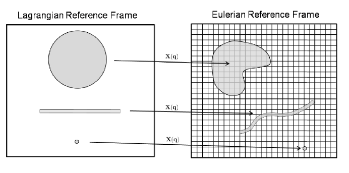
The basic Eulerian-Lagrangian formalism describing the state of the fluid and microstructures is given by the following equations

$$\frac{D\mathbf{p}(\mathbf{x},t)}{Dt} = \nabla\cdot\boldsymbol{\sigma}(\mathbf{x},t)+\Lambda(\mathbf{x},t)+\lambda(\mathbf{x},t)+\mathbf{g}(\mathbf{x},t)$$ (1)

$$\frac{\partial\mathbf{X}(\mathbf{q},t)}{\partial t} = \Gamma(\mathbf{q},t)+\gamma(\mathbf{q},t)+\mathbf{Z}(\mathbf{q},t).$$ (2)

The $\mathbf{p}$ accounts for the momentum of the material occupying location $\mathbf{x}$ and ${D\mathbf{p}}/{Dt}$ denotes the material derivative. The $\mathbf{X}(\mathbf{q},t)$ denotes the configuration of the material at time $t$ and parameterized by $\mathbf{q}$. The local material stress is denoted by $\boldsymbol{\sigma}=\boldsymbol{\sigma}[\mathbf{p},\mathbf{X}]$. We use the convention that $\boldsymbol{\sigma}$ accounts only for the dissipative stress contributions in the system. The operators $\Lambda$, $\Gamma$ couple the Eulerian and Lagrangian descriptions of the state of the material. The operator $\Lambda=\Lambda[\mathbf{X}]$ accounts for momentum gained or lost locally in the system as the material deforms from non-dissipative stresses and body forces. The operator $\Gamma=\Gamma[\mathbf{p},\mathbf{X}]$ determines the rate of deformation of the material from the momentum of the system. The $\lambda=\lambda[\mathbf{X},\mathbf{p}]$ and $\gamma=\gamma[\mathbf{X},\mathbf{p}]$ are Lagrange multipliers associated with time-independent kinematic constraints imposed on the system, such as rigidity of a body or incompressibility. Thermal fluctuations are taken into account through the stochastic fields $\mathbf{g}$ and $\mathbf{Z}$.

We consider systems where the total energy is given by

$$E[\mathbf{p},\mathbf{X}]=\int\frac{\rho_{0}}{2}|\mathbf{u}(\mathbf{x})|^{2}d\mathbf{x}+\Phi[\mathbf{X}],$$ (3)

where $\mathbf{u}(\mathbf{x})=\rho_{0}^{-1}\mathbf{p}(\mathbf{x})$ is the velocity of the material at location $\mathbf{x}$, $\rho_{0}$ is the constant mass density of the material, and $\Phi$ is the potential energy for a given configuration. The force associated with this energy is denoted by $\mathbf{F}=-\delta\Phi/\delta\mathbf{X}$.

For the operators which couple the Eulerian and Lagrangian descriptions to be physically consistent, the following should hold: (i) the coupling operators should not introduce any loss or gain of energy, (ii) momentum should only change through forces acting within the system. More precisely, these conditions require

$$\int\mathbf{F}(\mathbf{q})\cdot\Gamma(\mathbf{q})d\mathbf{q} = \int\left[\rho_{0}^{-1}\mathbf{p}(\mathbf{x})\right]\cdot\Lambda[\mathbf{F}](\mathbf{x})d\mathbf{x}$$ (4)

$$\int_{\Omega}\Lambda[\mathbf{F}](\mathbf{x})d\mathbf{x} = \int\mathbf{F}(\mathbf{q})d\mathbf{q}.$$ (5)

The conditions are required to hold for any realization of $\mathbf{X}$, $\mathbf{p}$, and $\mathbf{F}$. The condition 4 ensures the coupling operators conserve energy. The condition 5 ensures that in the absence of constraints the total momentum change of the system is equal to the total force acting on the system.

In the notation, we find it convenient to write the operator $\Lambda$ as explicitly depending on both $\mathbf{X}$ and $\mathbf{F}$, which for conservative forces is technically redundant. To simplify the discussion, it has been assumed that the stress contributions denoted by $\boldsymbol{\sigma}$ are entirely dissipative and that there is no net in-flux of momentum from boundary stresses $\int_{\partial\Omega}\boldsymbol{\sigma}(\mathbf{x})\cdot\mathbf{n}d\mathbf{x}=0$.

With these conditions satisfied by the coupling operators, we discuss how to account for thermal fluctuations using the stochastic fields $\mathbf{g}$ and $\mathbf{Z}$. It is convenient when accounting for thermal fluctuations to introduce coupling operators so that all configurations $\mathbf{X}$ are equally probable at statistical steady-state, when the $\Phi[\mathbf{X}]\equiv 0$. It can be shown that this corresponds to dynamics determined by the constraints and coupling operators which introduces an incompressible flow on phase space. The requirement of an incompressibile flow on phase space can be expressed as

$$\int\frac{\delta\Lambda}{\delta\mathbf{p}}(\mathbf{x},\mathbf{x})d\mathbf{x}+\int\frac{\delta\lambda}{\delta\mathbf{p}}(\mathbf{x},\mathbf{x})d\mathbf{x}+\int\frac{\delta\Gamma}{\delta\mathbf{X}}(\mathbf{q},\mathbf{q})d\mathbf{q}+\int\frac{\delta\gamma}{\delta\mathbf{X}}(\mathbf{q},\mathbf{q})d\mathbf{q} = 0.$$ (6)

This condition can be relaxed to allow for more general choices of coordinates, coupling operators, and constraints. If this condition is not satisfied a more general treatment of the thermal fluctuations is required to take into account in the invariant distribution the local compression or dilation of volume under the phase space flow [Tuckerman1999, ].

To simplify the discussion, we assume that the dissipative processes can be accounted for by a negative definite self-adjoint linear operator $\mathcal{L}$ in $\mathbf{p}$, so that $\nabla\cdot\boldsymbol{\sigma}=\mathcal{L}\mathbf{p}$, and that conditions 4 - 6 are satisfied. With these assumptions, the thermal fluctuations can be accounted for using for $\mathbf{g}$ and $\mathbf{Z}$ Gaussian stochastic fields which are mean zero and $\delta$-correlated in time [Oksendal2000, ; Gardiner1985, ]. The main issue then becomes to determine an appropriate spatial covariance structure for these stochastic fields. By requiring that the Boltzmann distribution be invariant under the stochastic dynamics of equations 1 - 2, it is required that $\mathbf{Z}=0$, and that

$$G(\mathbf{x},t,\mathbf{y},s)=\langle(\mathbf{g}(\mathbf{x},t))(\mathbf{g}(\mathbf{y},s))^{T}\rangle=-2k_{B}{T}\rho_{0}\delta(t-s)\mathcal{L}\delta(\mathbf{x}-\mathbf{y}),$$ (7)

see Appendix A.

Similar formulations as equations 1 - 2, with $\mathbf{g}=0$, $\mathbf{Z}=0$, are the starting point for the derivation of a wide variety of computational approaches used for systems in which fluids interact with rigid or elastic bodies. These include Arbitrary Lagrangian-Eulerian Methods (ALE) [Donea1983, ; Donea2004, ], Fluctuating Immersed Material (FIMAT) Dynamics [Patankar2004, ], Immersed Finite Element Methods (IFEM) [Wang2009, ; Zhang2004, ], and Immersed Boundary Methods (IBM) [Atzberger2007a, ; Peskin2002, ]. The approaches we introduce allow for the incorporation and simulation of thermal fluctuations in such methods, which collectively we refer to as Stochastic Eulerian-Lagrangian Methods (SELMs).

3 Semi-Discretization of the Momentum Equations, Microstructures, and the Eulerian-Lagrangian Coupling

We now consider semi-discretizations of the SELM equations. The momentum equations will be spatially discretized on a uniform mesh. The $\mathbf{p}_{\mathbf{m}}$ will denote the momentum at the mesh site indexed by $\mathbf{m}=(m_{1},m_{2},m_{3})$ and the composite vector of such values will be denoted by $\mathbf{p}$. The deformation state which describes the microstructure configurations will be discretized using a finite number of degrees of freedom denoted by $\mathbf{X}^{[j]}$ indexed by $j=0,1,\ldots,M$ and the composite vector denoted by $\mathbf{X}$. As an energy for this discretized system we use

$$E[\mathbf{p},\mathbf{X}]=\sum_{\mathbf{m}}\frac{1}{2}\rho_{0}^{-1}|\mathbf{p}_{\mathbf{m}}|^{2}\Delta{x}^{d}+\Phi(\mathbf{X})$$ (8)

where $\Delta{x}$ is the mesh spacing and $d$ is the number of dimensions. The semi-discretization in space of the momentum and configuration equations can be expressed as

$$\frac{\tilde{D}\mathbf{p}}{\tilde{D}t} = L\mathbf{p}+\Lambda+\lambda+\mathbf{g}$$ (9)

$$\frac{\partial\mathbf{X}^{[j]}(t)}{\partial t} = \Gamma^{[j]}+\gamma^{[j]}$$ (10)

where ${\tilde{D}}/{\tilde{D}t}$ and $L$ denote respectively the spatially discretized approximation of the material derivative and $\mathcal{L}$. The $\mathbf{p}$, $\Lambda$, $\lambda$, $\mathbf{g}$ denote the composite vector of values on the mesh and $\mathbf{X}^{[j]}$, $\Gamma^{[j]}$, $\gamma^{[j]}$ denote values associated with the $j^{th}$ configurational degree of freedom. We assume the discrete dissipative operator is symmetric $L=L^{T}$ and negative semi-definite. For the coupling operators of the discretized equations the corresponding consistency conditions 4 - 5 are

$$\Gamma[\mathbf{p}]^{T}\mathbf{F} = \rho_{0}^{-1}\mathbf{p}^{T}\Lambda[\mathbf{F}]\Delta{x}^{d}$$ (11)

$$\sum_{\mathbf{m}}\Lambda[\mathbf{F}]_{\mathbf{m}}\Delta{x}^{d} = \sum_{j}\mathbf{F}^{[j]}.$$ (12)

The superscript T denotes the matrix transpose. The first condition ensures for the discretized system that the coupling preserves the energy and the second that changes in momentum only occur from forces acting within the system. The phase space incompressibility condition corresponding to equation 6 in the discretized setting becomes

$$\nabla_{\mathbf{p}}\cdot(\Lambda+\lambda)+\nabla_{\mathbf{X}}\cdot(\Gamma+\gamma) = 0.$$ (13)

This condition ensures the uniform distribution for the configurations $\mathbf{X}$ is invariant under the stochastic dynamics of equation 9-10 when the potential energy is constant, i.e. $\Phi\equiv 0$. When $\Lambda$ and $\Gamma$ are linear operators the energy condition 4 amounts to the coupling operators being adjoints (up to a scalar),

$$\Gamma=\Lambda^{T}\rho_{0}\Delta{x}^{d}.$$ (14)

Provided conditions 11 - 13 are satisfied, the thermal fluctuations can be taken into account using a Gaussian stochastic field on the lattice, without any direct stochastic forcing required in the microstructure equations 2. If these conditions are violated by the discretization the numerical approximation may introduce artificial loss or gain of energy or momentum in the system. In order to be consistent with the fluctuation-dissipation principle of statistical mechanics such discretizations would require additional sources of stochastic forcing to obtain the appropriate Boltzmann ensemble.

An appropriate covariance structure for the stochastic driving field for discretizations satisfying conditions 11 - 13 can be determined by requiring invariance of the Boltzmann distribution under the stochastic dynamics of equation 9 - 10. This yields for the semi-discrete system, see Appendix A,

$$G=\langle\mathbf{g}\mathbf{g}^{T}\rangle=-2LC.$$ (15)

The covariance of the equilibrium fluctuations is given by the entries

$$C=\frac{\rho_{0}{k_{B}{T}}}{\Delta{x}^{d}}I,$$ (16)

where $I$ is the identity matrix, see Appendix A.

One such realization of this SELM approach is the Stochastic Immersed Boundary Method developed in [Atzberger2007a, ]. In this case the coupling operators are given by

$$\Lambda_{IB}\mathbf{F} = \sum_{j=1}^{M}\mathbf{F}^{[j]}(\mathbf{X}(t))\delta_{a}(\mathbf{x}_{\mathbf{m}}-\mathbf{X}^{[j]}(t))$$ (17)

$$\left[\Gamma_{IB}\mathbf{u}\right]^{[j]} = \sum_{\mathbf{m}}\delta_{a}(\mathbf{x}_{\mathbf{m}}-\mathbf{X}^{[j]}(t))\mathbf{u}_{\mathbf{m}}(t)\Delta{x}^{d}.$$ (18)

where $\mathbf{u}=\rho_{0}^{-1}\mathbf{p}$, and $\delta_{a}$ is a special kernel function approximating the Dirac $\delta$-function, see Appendix C. The dynamics are subject to the constraint that the fluid is incompressible $\nabla\cdot\mathbf{u}=0$. For the semi-discretized SIB method of [Atzberger2007a, ] the conditions 11 and 12 can be readily verified to hold exactly. However, the condition 13 only approximately holds and is exact only in the continuum limit. As $\Delta{x}\rightarrow 0$ we have

$$\nabla_{\mathbf{X}^{[j]}}\cdot\Gamma = \sum_{\mathbf{m}}-\nabla\delta_{a}(\mathbf{x}_{\mathbf{m}}-\mathbf{X}^{[j]})\mathbf{u}_{\mathbf{m}}\Delta{x}^{d}\rightarrow\int-\nabla\delta_{a}(\mathbf{y}-\mathbf{X}^{[j]})\mathbf{u}({\mathbf{y}})d\mathbf{y}$$

$$= \int\delta_{a}(\mathbf{y}-\mathbf{X}^{[j]})\nabla\cdot\mathbf{u}({\mathbf{y}})d\mathbf{y}=0.$$

In the last line we used that the fluid is incompressible $\nabla\cdot\mathbf{u}=0$. The divergence of the terms $\Lambda$, $\lambda$, $\gamma$, are zero in this case. In practice, the method still yields reasonable results since the exhibited fluctuations deviate from Boltzmann statistics only up to the discretization error [Atzberger2007a, ; Atzberger2008, ].

4 Soft Materials and Complex Fluids Subject to Shear

We now discuss how the SELM approach can be used for the study of rheological properties of soft materials and complex fluids. We then discuss specific stochastic numerical methods for performing simulations in practice. For the type of materials we consider, it will be assumed that the solvent hydrodynamics is described well by the constitutive laws of Newtonian fluids in the physical regime where the Reynolds number is small. We also assume that the explicitly represented microstructures occupy only a relatively small volume fraction and are effectively density matched with the solvent fluid. In this regime, the momentum of the system will be accounted for using the time-dependent Stokes equations

$$\rho_{0}{\frac{\partial\mathbf{u}}{\partial t}} = \mu{\Delta}{\mathbf{u}}-\nabla{p}+\Lambda+\mathbf{g}$$ (20)

$$\nabla\cdot{\mathbf{u}} = 0$$ (21)

where $\mathbf{u}(\mathbf{x},t)=\rho_{0}^{-1}\mathbf{p}(\mathbf{x},t)$ is the local velocity of the fluid body at $\mathbf{x}$ in the Eulerian reference frame, $\rho_{0}$ is the fluid density, $\mu$ is the dynamic viscosity, and $p$ is the pressure. This corresponds to the dissipative stress $\boldsymbol{\sigma}=\mu\left(\nabla\mathbf{u}+\nabla\mathbf{u}^{T}\right)$ and $\lambda=-\nabla{p}$ in equation 1. While the Reynolds number is small, the partial time derivative is retained in the Stokes flow in equation 20 since the thermal fluctuations introduce small characteristic time scales into the dynamics.

To introduce shear we generalize the usual periodic boundary conditions. Our basic approach is motivated by the molecular dynamics methods introduced by Lees-Edwards [LeesEdwards1972, ; Evans1979, ; EvansMorriss1984, ]. In this work, molecules in the base unit cell have modified interactions with molecules in periodic images. To simulate a bulk material undergoing a shear deformation at a given rate, the periodic images are treated as shifting in time relative to the unit cell, see Figure 2. This has the effect of modifying both the location of periodic images of molecules and their assigned velocities. This has some advantages over other approaches, where an affine-like deformation is imposed on the entire material body [EvansMorriss1990, ; Hoover1980, ; Hoover2008, ]. In contrast, for the Lees-Edwards approach the shear deformation is only imposed at the boundaries allowing within the unit cell for the molecular interactions to determine the form of the shear response.

Motivated by this molecular dynamics condition we develop a corresponding methodology for the SELM approach. For momentum accounted for by the time-dependent Stokes equations we introduce the following generalized periodic boundary conditions

$$\mathbf{u}(x,y,L,t)=\mathbf{u}(x-vt,y,0,t)+v\mathbf{e}_{x}.$$ (22)

For concreteness we consider the case where a shear is imposed in the z-direction giving rise to velocities in the x-direction. The $L$ is the side length of the periodic cell in the z-direction, $v=L\dot{\gamma}$ is the velocity of the top face of the unit cell relative to the bottom face, $\dot{\gamma}$ denotes the rate of shear deformation, and $\mathbf{e}_{j}$ is the standard unit vector in the $j^{th}$ direction. The interactions between microstructures of the system can be readily handled in the same manner as in the molecular dynamics simulation. This is done by shifting the location of any microstructure of a periodic image involved in an interaction.

While conceptually straight-forward, these boundary conditions present significant challenges in practice for the numerical discretization of the momentum equations. The conditions introduce both a jump discontinuity at periodic boundaries and a shift which potentially leads to misalignment of discretization nodes at the domain boundaries, see Figure 2. For commonly employed approaches such as spectral Fourier methods the jump discontinuity results in a degradation of accuracy through the resulting Gibbs’ phenomena [Goldberg1976, ]. For uniform finite difference methods on the unit cell the mesh misalignment requires modified stencils or interpolations at the domain boundary. When incorporating stochastic driving fields to account for thermal fluctuations these issues are further compounded.

Fig. 2: Discretization Mesh with Lees-Edwards Boundary Conditions Initial Formulation. The boundary conditions induce shear by shifting the periodic images of the unit cell, shown on the left and middle. For uniform discretizations of the unit cell this presents challenges since the mesh becomes misaligned at boundaries between the unit cell and the periodic images, shown on the right.

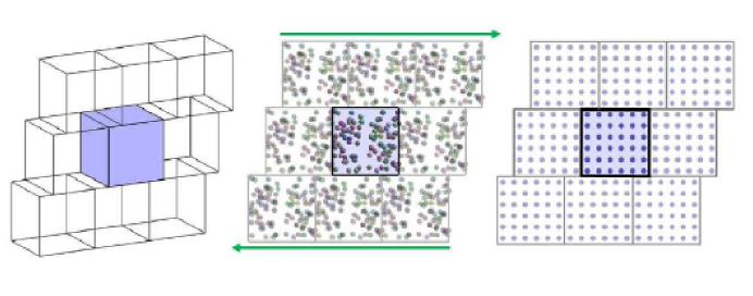
To address these issues, we develop discretization methods which utilize a moving coordinate frame which deforms with the unit cell, see Figure 3. Let the velocity field in this frame be denoted by $\mathbf{w}(\mathbf{q},t):=\mathbf{u}(\phi(\mathbf{q},t),t)$, where $\mathbf{q}=(q_{1},q_{2},q_{3})$ parameterizes the deformed unit cell. Let $\phi(\mathbf{q},t)=(q_{1}+q_{3}\dot{\gamma}t,q_{2},q_{3})$ denote the map from the moving coordinate frame to the fixed Eulerian coordinate frame $\mathbf{x}=\phi(\mathbf{q})$. The time-dependent Stokes equations in the deforming coordinate frame become

$${\frac{d\mathbf{w}^{(d)}}{dt}} = \rho_{0}^{-1}\mu\left[\mathbf{e}_{d}-\delta_{d,3}\dot{\gamma}t\mathbf{e}_{x}\right]^{T}\nabla^{2}\mathbf{w}^{(d)}\left[\mathbf{e}_{d}-\delta_{d,3}\dot{\gamma}t\mathbf{e}_{x}\right]-\nabla{p}+\mathbf{F}+\mathbf{J}$$ (23)

$$\nabla\cdot\mathbf{w} - \mathbf{e}_{z}^{T}\hskip 2.84544pt\nabla\mathbf{w}\hskip 2.84544pt\mathbf{e}_{x}\dot{\gamma}t=\mathbf{K}$$ (24)

where $\mathbf{q}=(q_{1},q_{2},q_{3})$ parameterizes the deformed unit cell, $\dot{\gamma}$ denotes the rate of the shear deformation, $\mathbf{e}_{i}$ the standard basis vector in the $i$ direction with $i\in\{x,y,z\}$. In the notation the parenthesized superscript denotes a vector component and $\delta_{k,\ell}$ denotes the Kronecker $\delta$-function. We also use the notational convention

$$\left[\nabla^{2}\mathbf{w}^{(d)}\right]_{i,j} = \frac{\partial^{2}\mathbf{w}^{(d)}}{\partial q_{i}\partial q_{j}}$$ (25)

$$\left[\nabla\mathbf{w}\right]_{d,j} = \frac{\partial\mathbf{w}^{(d)}}{\partial q_{j}}.$$ (26)

In the equations, the terms $\mathbf{J},\mathbf{K}$ are introduced to account for the jump introduced by the boundary conditions 22. This allows in the new coordinate frame for use of the usual periodic boundary conditions

$$\mathbf{w}(q_{1},q_{2},L,t)=\mathbf{w}(q_{1},q_{2},0,t).$$ (27)

Fig. 3: Discretization Mesh with Lees-Edwards Boundary Conditions Using a Moving Coordinate Frame. By discretizing the momentum equations in a moving coordinate frame a uniform discretization is obtained in which the mesh of the unit cell aligns with the mesh of the periodic images, shown on the left, middle, and right. The definition of the unit cell is changed from a cube to a sheared parallelepiped, shown on the far right on the bottom.

We now discuss a discretization for equations 23 and 24 and the corresponding source terms $\mathbf{J},\mathbf{K}$. The following central finite difference approximations will be used

$$\frac{\partial\mathbf{w}^{(d)}}{\partial q_{i}} \rightarrow \frac{\mathbf{w}^{(d)}(\mathbf{q}+\mathbf{e}_{i})-\mathbf{w}^{(d)}(\mathbf{q}-\mathbf{e}_{i})}{2\Delta{x}}$$ (28)

$$\frac{\partial^{2}\mathbf{w}^{(d)}}{\partial q_{i}\partial q_{j}} \rightarrow \frac{\mathbf{w}^{(d)}(\mathbf{q}+\mathbf{e}_{i}+\mathbf{e}_{j})-\mathbf{w}^{(d)}(\mathbf{q}-\mathbf{e}_{i}+\mathbf{e}_{j})}{4\Delta{x}^{2}}$$

$$- \frac{\mathbf{w}^{(d)}(\mathbf{q}+\mathbf{e}_{i}-\mathbf{e}_{j})-\mathbf{w}^{(d)}(\mathbf{q}-\mathbf{e}_{i}-\mathbf{e}_{j})}{4\Delta{x}^{2}},\mbox{ $i\not=j$}$$

$$\frac{\partial^{2}\mathbf{w}^{(d)}}{\partial q_{i}^{2}} \rightarrow \frac{\mathbf{w}^{(d)}(\mathbf{q}+\mathbf{e}_{i})-2\mathbf{w}^{(d)}(\mathbf{q})+\mathbf{w}^{(d)}(\mathbf{q}-\mathbf{e}_{i})}{\Delta{x}^{2}}.$$ (30)

These approximations are substituted into equations 25–26 to approximate the operators in equation 23–24.

We remark that the moving coordinate frame makes the description of the momentum field have some features of a Lagrangian frame of reference. We none-the-less retain the Eulerian terminology treating this distinction loosely since the deformation corresponds to a somewhat arbitrary coordinate frame introduced for numerical convenience and does not directly follow from the details of the fluid flow. Our discretization approach shares features with Arbitrary Eulerian Lagrangian (ALE) Methods [Donea1983, ; Donea2004, ].

An important issue when using such deforming reference frames is that the discretization stencils may become excessively distorted [Donea1983, ; Donea2004, ]. We avoid this issue by exploiting the periodic symmetry of the system in the $x$ and $y$ directions. Let the displacement in the $x$-direction of the top of the unit cell relative to the bottom of the unit cell be denoted by $s$. For shear rate $\dot{\gamma}$ and cell size $L$ the displacement at time $t$ is given by $s=L\dot{\gamma}t$. The periodicity in the $x$ and $y$ directions has the consequence that for any coordinate frame with $s>L$ there is another coordinate frame with $s<L$ which has aligned mesh sites, see Figure 3. By adopting the convention that the coordinate frame with $s<L$ is always used when evaluating stencils the distortion is controlled.

To obtain approximations for the source terms $\mathbf{J},\mathbf{K}$ the discretization stencils are applied at the shear boundaries of the unit cell. For any stencil weights involving values at mesh sites which cross the boundary the modified image value is used $\mathbf{w}_{\mathbf{m}}\pm\dot{\gamma}L$. The contributions of the stencil weights multiplied by $\pm\dot{\gamma}L$ are collected over all boundary mesh sites to obtain the source terms $\mathbf{J}$, $\mathbf{K}$. This allows for the usual finite difference stencils to be used on the unit cell with regular periodic boundary conditions. When including the source terms this gives the equivalent result of imposing the jump boundary condition 22. This formulation has a number of advantages when numerically solving the discretized equations and when introducing thermal fluctuations.

The Stokes equations 23– 24 discretized in this manner on a uniform periodic mesh can be expressed as

$${\frac{\partial\mathbf{w}}{\partial t}} = L(t)\mathbf{w}+\mathbf{F}+\mathbf{J}+\mathbf{g}$$ (31)

$$D(t)\mathbf{w} = \mathbf{K}$$ (32)

where $L(t)$ denotes the finite difference operator approximating the Laplacian in the moving coordinate frame, and $D(t)$ the approximation of the Divergence operator in the moving frame, see equation 24. The discretization $L(t)$ can be shown to be symmetric and negative semi-definite for each $t$.

An important property of $L(t),D(t)$ is that for each time $t$ the corresponding stencils are translation invariant with respect to lattice shifts of the mesh. This has the important consequence that the matrix representations are circulant and therefore diagonalizable by Fast Fourier Transforms [Strang1988, ]. As a result, the incompressibility constraint can be handled using FFTs to obtain an exact projection method [Chorin1968, ]. This allows for the discretized approximation of the Stokes equations to be expressed as

$${\frac{\partial\mathbf{w}}{\partial t}} = \wp(t)\left[L(t)\mathbf{w}+\mathbf{F}+\mathbf{J}\right]+\mathbf{g}$$ (33)

where $\wp(t)$ is the operator which projects to the null space of $D(t)$. The incompressibility condition is then satisfied for all time provided $D(0)\cdot\mathbf{w}(0)=\mathbf{K}$.

We discuss stochastic numerical methods for two particular physical regimes: (i) the relaxation of the hydrodynamic modes of the system is resolved explicitly, (ii) for the current configuration $\mathbf{X}$ the hydrodynamic modes are treated as having relaxed to statistical steady-state. We remark that the case of resolving the hydrodynamic relaxation of the system is amenable to stochastic numerical methods similar to those introduced in [Atzberger2007a, ]. We discuss this case only briefly and focus primarily on the newly introduced stochastic numerical methods for handling the second case.

5 Regime I : Resolution of Hydrodynamic Relaxation

We now discuss in practice how the stochastic fields may be generated in the regime where the relaxation of the hydrodynamic modes is resolved explicitly. For this purpose we express equation 33 in differential form

$$d\mathbf{w} = \wp(t)\left[L(t)\mathbf{w}+\mathbf{F}+\mathbf{J}\right]dt+Qd\mathbf{B}_{t}.$$ (34)

The $Qd\mathbf{B}_{t}$ denotes the stochastic driving field accounting for thermal fluctuations corresponding to $\mathbf{g}$ and $\mathbf{B}_{t}\in\mathbb{R}^{3N}$ denotes the composite vector of a standard Brownian motion process at each of the mesh sites. Throughout our discussion the stochastic differential equations will be given the Ito interpretation [Gardiner1985, ].

Using $\langle Qd\mathbf{B}_{t}d\mathbf{B}_{t}^{T}Q^{T}\rangle=QQ^{T}dt=Gdt$, we see that $Q$ denotes a matrix square-root of the covariance of the stochastic driving field $G=QQ^{T}$. Given the discretizations introduced in Section 4, the dissipative operator $L(t)$ depends on time, which requires, see Appendix B,

$$G(t)=-2\wp(t)L(t)C.$$ (35)

This has the consequence that the covariance of the stochastic driving field is time dependent.

In the discretized system the numerical stencils dependent on time, However, since the shear deformation is volume preserving the discretized summation introduced to model the kinetic energy of the discrete system in equation 8 evaluated in the deformed coordinates is in fact not dependent on time. Since we made this choice, we have the important consequence that the Boltzmann equilibrium fluctuations of the velocity field $\mathbf{w}$ associated with this energy are stationary (independent of time). In other words, the covariance $C$ of the equilibrium fluctuations on the discretized lattice for the energy given in equation 8 is independent of time, $C(t)=C(0)$. This holds even though the underlying discretization and corresponding operators $L(t)$, $\wp(t)$, $G(t)$ depend on time.

To obtain an explicit form for $G(t)$ we need to compute $C$ taking into account the incompressibility constraint 32. The equilibrium covariance under these constraints is given by

$$C=\frac{2}{3}\frac{k_{B}{T}}{\rho_{0}\Delta{x}^{d}}I.$$ (36)

The factor ${2}/{3}$ arises from application in Fourier space of the projection operator which equivalently enforces the incompressibility. The factor $\rho_{0}$ appears in the denominator since the velocity $\mathbf{w}$ is considered, instead of the momentum $\mathbf{p}=\rho_{0}\mathbf{w}$. The notation for the stochastic driving field $\mathbf{g}$ is used loosely when switching between the momentum and velocity equations.

The time dependent covariance structure of the stochastic driving field $\mathbf{g}$ in equation 34 is of the form $G(t)=-2\wp(t){L}(t)C$. An important issue is whether this will indeed yield a consistent treatment of the thermal fluctuations so that the resulting stochastic dynamical system has the required equilibrium fluctuations. We establish a Fluctuation-Dissipation principle for such time dependent systems in Appendix B.

6 Generating the Stochastic Driving Field I

In order for equation 35 and 36 to be useful in practice, we must have efficient methods by which to generate the stochastic driving fields with the required covariance structure. A significant challenge in practice is to generate efficiently the Gaussian stochastic driving field with the required covariance structure $G(t)$. A commonly used approach is to generate a variate with uncorrelated standard Gaussian components $\boldsymbol{\xi}$ and set $\mathbf{g}=Q(t)\boldsymbol{\xi}$ for an appropriately chosen matrix $Q(t)$. The resulting variate $\mathbf{g}$ then has covariance $\langle\mathbf{g}\mathbf{g}^{T}\rangle=Q(t)\langle\boldsymbol{\xi}\boldsymbol{\xi}^{T}\rangle Q(t)^{T}=Q(t)Q(t)^{T}=G(t)$, with a proper choice of $Q(t)$.

However, to carry this out in practice encounters two challenges: (i) given $G(t)$ the factor $Q(t)$ must be determined, (ii) the matrix-vector multiplication $Q(t)\boldsymbol{\xi}$ must be carried out. For (i) the Cholesky algorithm is typically used with a computational cost of $O(N^{3})$, where $N$ is the number of components of $\mathbf{g}$. For (ii) the resulting factors $Q(t)$ are generally not sparse, which when generating each variate incurs a computational cost of $O(N^{2})$. To get a sense of the costs, for a three dimensional mesh, the number of components of $\mathbf{g}$ scales cubically as $N=(\ell/\Delta{x})^{3}$, where $\ell$ is the domain size and $\Delta{x}$ is the mesh resolution. The associated costs for generating the variates using this approach even for moderate spatial resolutions is prohibitively expensive.

To obtain a more efficient computational method we use specific features of the discretization introduced in Section 4. One useful feature of the discretization we use is that the equilibrium covariance matrix is proportional to the identity matrix $C=\alpha\mathcal{I}$ with $\alpha={2k_{B}{T}}/{3\rho_{0}\Delta{x}^{d}}$. This allows equation 35 to be expressed as

$$G(t)=-2\alpha\wp(t)L(t).$$ (37)

We also use the following specific properties of the operators $C$, $L(t)$, and $\wp(t)$ obtained from the discretization. The first is that each of the operators corresponds to use of numerical stencils which are translation invariant on the mesh. This has the important consequence that all of these operators are diagonalizable in the Fourier basis. This has the further important consequence that all of these operators commute. The second is that $\wp$ is an exact projection operator, so that $\wp^{2}=\wp$ and $\wp=\wp^{T}$. Finally, we use that the discrete approximation of the Laplacian is symmetric negative semi-definite so that it can be factored as $L(t)=-U(t)U^{T}(t)$ for some matrix $U(t)$.

By using these properties of the operators we can express the covariance of the stochastic driving field as

$$G(t)=\left(\sqrt{2\alpha}\wp U(t)\right)\left(\sqrt{2\alpha}\wp U(t)\right)^{T}.$$ (38)

In this form the required matrix square-root is readily obtained as $Q(t)=\sqrt{2\alpha}\wp U(t)$. We remark this is different than the Cholesky factor obtained from $G(t)$ which is required to be lower triangular [Trefethen1997, ]. Since the operators $L(t)$ and $\wp$ are diagonalizable in Fourier space, the matrix action of the operators $U(t)$ and $\wp$ on any vector can be computed using the Fast Fourier Transform with a cost of $O(N\log(N))$. In summary, our method allows in practice for the random variates of the stochastic driving field to be computed from $\mathbf{g}=Q(t)\boldsymbol{\xi}$ very efficiently, with a computational cost of only $O(N\log(N))$. This is in contrast to the traditional Cholesky approach with a computational cost of $O(N^{3})$.

7 Regime II : Under-resolution of Hydrodynamic Relaxation (Quasi-Steady-State Limit)

For many problems the equations of motion can be simplified by exploiting a separation of time-scales between the time-scale on which the hydrodynamic modes relax to a statistical steady-state and the time-scale associated with the motion of the microstructures. In this case the fluid equations can be approximated by

$$\mathbf{w}=-\tilde{L}(t)^{-1}\left[\Lambda+\mathbf{J}\right]+\mathbf{a}.$$ (39)

The $\tilde{L}=\wp L\wp^{T}$ and the inverse is defined for the operator restricted to the linear space $\mathcal{V}=\{\mathbf{w}\in\mathbb{R}^{3N}|\wp\mathbf{w}=\mathbf{w}\}$. The term $\mathbf{a}$ is introduced to account for the thermal fluctuations in this regime. We refer to this as the Quasi-Steady-State Stokes approximation [Brady1988, ]. Using this in equation 10, we obtain the following closed system of equations for the motion of the microstructures

$$\frac{d\mathbf{X}(t)}{dt}=H_{\mbox{\tiny SELM}}(t)\left[\mathbf{F}\right]+\bar{\mathbf{J}}+\mathbf{A}$$ (40)

where

$$H_{\mbox{\tiny SELM}}(t) = -\Gamma\tilde{L}(t)^{-1}\Lambda$$ (41)

$$\bar{\mathbf{J}} = -\Gamma\tilde{L}(t)^{-1}\mathbf{J}.$$ (42)

The $\mathbf{A}$ will be used to account for the thermal fluctuations. We consider the specific case when the operator $\Lambda$ is linear in $\mathbf{F}$ and $\Gamma$ is linear in $\mathbf{u}$. In this case $H_{\mbox{\tiny SELM}}$ is a tensor which we refer to as the ”effective hydrodynamic coupling tensor.”

In this regime the thermal fluctuations arise from the hydrodynamic modes which are relaxed to statistical steady-state. A key challenge is to determine the appropriate statistics of $\mathbf{A}$ which accounts for the time integrated thermal fluctuations of the hydrodynamics which impact the microstructure dynamics. For this purpose we rewrite equation 40 in differential form as

$$d\mathbf{X}(t)=H_{\mbox{\tiny SELM}}(t)\mathbf{F}dt+R(t)d\mathbf{B}_{t}$$ (43)

neglecting for the moment $\bar{\mathbf{J}}$, and representing the contributions of $\mathbf{A}$ by $R(t)d\mathbf{B}_{t}$. We derive the covariance structure $S(t)=R(t)R(t)^{T}$ by requiring consistency with the principle of Detailed-Balance of statistical mechanics [Reichl1998, ]. The Fokker-Planck equation associated with equation 43 is

$$\frac{\partial\Psi(\mathbf{X},t)}{\partial t} = -\nabla\cdot\mathcal{J}$$ (44)

$$\mathcal{J} = H_{\mbox{\tiny SELM}}(t)\mathbf{F}\Psi-\frac{1}{2}S(t)\nabla_{\mathbf{X}}\Psi.$$ (45)

The $\Psi(\mathbf{X},t)$ is the probability density for the microstructures to have configuration $\mathbf{X}$ at time $t$. The equilibrium fluctuations of the system are required to have the Boltzmann distribution

$$\Psi_{BD}(\mathbf{X})=\frac{1}{Z}\exp\left(-\Phi(\mathbf{X})/k_{B}T\right)$$ (46)

where $Z$ is a normalization constant which ensures the distribution integrates to one [Reichl1998, ]. Substituting this above and using that $H_{\mbox{\tiny SELM}}$ is linear in $\mathbf{F}$ gives

$$\mathcal{J} = \left(H_{\mbox{\tiny SELM}}(t)-\frac{1}{2k_{B}T}S(t)\right)\mathbf{F}\Psi_{BD}$$ (47)

where $\mathbf{F}=-\nabla_{\mathbf{X}}{\Phi}$. The principle of Detailed-Balance requires at thermodynamic equilibrium that $\mathcal{J}=0$. Requiring this to hold for all possible $\mathbf{F}$ gives

$$S(t)=2k_{B}TH_{\mbox{\tiny SELM}}(t).$$ (48)

For $S(t)$ to provide a covariance for a real-valued stochastic driving term, the hydrodynamic coupling tensor $H_{\mbox{\tiny SELM}}(t)$ must be symmetric and positive semi-definite. In the case that $\Lambda$ and $\Gamma$ are linear operators this is ensured by condition 11, which from expression 41 gives

$$\mathbf{q}^{T}H_{\mbox{\tiny SELM}}(t)\mathbf{q}=-\mathbf{v}^{T}\left(\tilde{L}(t)^{-1}\right)\mathbf{v}\Delta{x}^{d}\geq 0.$$ (49)

To obtain this result we let $\mathbf{v}=\Gamma^{T}\mathbf{q}$ and use that $\tilde{L}(t)^{-1}$ is symmetric negative definite. To obtain an approach useful in practice requires efficient methods for the generation of the stochastic driving term with covariance $S(t)$.

7.1 Generating the Stochastic Driving Field II

As discussed in Section 6, a significant challenge in practice is to generate efficiently the Gaussian stochastic driving terms with the required covariance structure. We discuss an approach for SELM methods when the coupling operators $\Lambda$ and $\Gamma$ are linear. In this case

$$H_{\mbox{\tiny SELM}}(t) = -\Gamma\tilde{L}(t)^{-1}\Gamma^{T}\Delta{x}^{d}$$ (50)

by condition 11. Using properties of the operators discussed in Section 4, we can express the hydrodynamic coupling tensor as

$$H_{\mbox{\tiny SELM}}(t) = \left(\Gamma(t)V(t)\Delta{x}^{d/2}\right)\left(\Gamma(t)V(t)\Delta{x}^{d/2}\right)^{T}.$$ (51)

We have used that the operators $L(t)$ and $\wp$ commute and since $\wp$ is an exact projection that $\wp=\wp^{T}$, $\wp=\wp^{2}$. Since $\tilde{L}(t)$ is symmetric negative definite on the linear space $\mathcal{V}=\{\mathbf{w}\in\mathbb{R}^{3N}|\wp\mathbf{w}=\mathbf{w}\}$, we can factor $\tilde{L}(t)^{-1}=-V(t)V(t)^{T}$. The factor $V(t)$ is readily obtained since $L(t)$ and $\wp$ are diagonalizable in the Fourier basis. From equations 51 and 48 we can factor the covariance as $S(t)=R(t)R(t)^{T}$ with

$$R(t)=\left(2k_{B}{T}\Delta{x}^{d}\right)^{1/2}\Gamma(t)V(t).$$ (52)

This expression for the factor can be used to compute the required Gaussian stochastic driving term $\mathbf{A}=R(t)\boldsymbol{\xi}$ with a computational cost of $O(N\log(N)+M)$, where $N$ is the total number of mesh sites in the momentum field discretization and assuming the action of $\Gamma$ can be computed with a cost of $O(M)$ with $M<N$.

The random variates are generated by utilizing the underlying discretization mesh of the momentum equations. This is accomplished by generating on the mesh uncorrelated standard Gaussian random variates $\boldsymbol{\xi}$. Since $V(t)$ is diagonal in the Fourier basis, the action $V(t)\boldsymbol{\xi}$ is computed in Fourier space with a cost of only $O(N\log(N))$. The operator $\Gamma$ is then applied. If the operator $\Gamma(t)$ makes use of only localized values of the mesh it can be computed with computational cost of $O(M)$. The last step in generating the random variate requires a scalar multiplication which incurs a computational cost of $O(M)$. This procedure generates the stochastic driving term $\mathbf{A}$ with a computational cost of $O(N\log(N)+M)$. For a sufficiently large number of microstructure degrees of freedom $M$, this method is significantly more efficient than the traditional approach based on Cholesky factorization of $H_{\mbox{\tiny SELM}}$ which costs $O(M^{3})$.

7.1.1 Effective Hydrodynamic Coupling Tensor : $\mathbf{H}_{\mbox{\tiny SELM}}$

We now discuss an approach for analyzing the effective hydrodynamic coupling tensors $\mathbf{H}_{\mbox{\tiny SELM}}$ which appear in the quasi-steady-state formulation of the SELM approach. From equation 41 many types of hydrodynamic coupling tensors are possible depending on the kinetic constraints and choice of coupling operators $\Lambda$ and $\Gamma$. For concreteness we discuss the specific case corresponding to the Stochastic Immersed Boundary Method (SIB) [Peskin2002, ; Atzberger2007a, ]. In the case of the SIB method, the specific coupling operators $\Lambda$ and $\Gamma$ are given by 17 and 18. From equation 41 the effective hydrodynamic coupling tensor is given by

$$\left[\mathbf{H}_{\mbox{\tiny IB}}(t)\left[\mathbf{F}\right]\right]^{[j]} = -\sum_{\mathbf{m}}\delta_{a}(\mathbf{x}_{\mathbf{m}}-\mathbf{X}^{[j]}(t))\left[\tilde{L}(t)^{-1}\left(\sum_{j=1}^{M}\mathbf{F}^{[j]}\delta_{a}(\mathbf{x}_{\mathbf{m}}-\mathbf{X}^{[j]}(t))\right)\right]_{\mathbf{m}}\Delta{x}^{d}.$$

In the notation, the superscript $[\cdot]^{[j]}$ denotes for the composite vector the components associated with the $j^{th}$ microstructure degree of freedom. The $[\cdot]_{\mathbf{m}}$ denotes the vector components associated with the mesh site with index $\mathbf{m}$. An analysis of variants of this tensor for point particles and slender bodies was carried-out in [Bringley2008, ; Atzberger2007c, ].

Since $\mathbf{H}_{\mbox{\tiny IB}}$ is linear in the microstructure forces, without loss of generality we can consider the case of only two microstructure degrees of freedom. We denote these as $\mathbf{X}^{[1]}$, $\mathbf{X}^{[2]}$ and the displacement vector by $\mathbf{z}=\mathbf{X}^{[2]}-\mathbf{X}^{[1]}$. In making comparisons with other hydrodynamic coupling tensors we find it helpful to make use of approximate symmetries satisfied by $\mathbf{H}_{\mbox{\tiny IB}}$. From equation LABEL:equ_def_H_IB, $\mathbf{H}_{\mbox{\tiny IB}}$ depends on $\mathbf{z}$ up to a shift of $\mathbf{X}^{[1]}$ relative to the nearest mesh site, and is similarly rotationally symmetry about the axis of $\mathbf{z}$. This allows the tensor components for all configurations to be related to a canonical configuration with $\mathbf{z}=(z_{1},0,0)$. For any configuration this is accomplished by introducing the rotation matrix $U$ so that $U\mathbf{z}=(z_{1},0,0)$ and considering $\tilde{\mathbf{H}}=U\mathbf{H}_{\mbox{\tiny IB}}U^{T}$. In our comparisons we consider $\bar{\mathbf{H}}_{\mbox{\tiny IB}}=\langle\tilde{\mathbf{H}}\rangle$, where the average is taken over all rotations and shifts with respect to the nearest mesh site.

Fig. 4: Comparison of the Hydrodynamic Coupling Tensor of the Immersed Boundary Method $\mathbf{H}_{\mbox{\tiny IB}}$ with the Oseen Tensor $\mathbf{H}_{\mbox{\tiny OS}}$ and the Rotne-Prager-Yamakawa Tensor $\mathbf{H}_{\mbox{\tiny RPY}}$. The components of the hydrodynamic coupling tensor for displacement $r=|\mathbf{z}|$ are shown for the parallel direction (circles) and the perpendicular direction (squares). For two particles subject to an equal and opposite force, the velocity field corresponding to the Rotne-Prager-Yamakawa Tensor is shown on the right. The lighter shaded regions indicate a larger magnitude of the velocity.

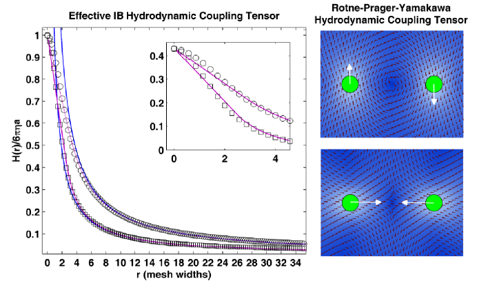
In practice, to numerically compute $\bar{\mathbf{H}}_{\mbox{\tiny IB}}$ we sample random configurations of $\mathbf{X}^{[1]}$ and $\mathbf{X}^{[2]}$. A useful expression for the tensor components is $H_{ij}=\mathbf{e}_{i}^{T}\mathbf{H}\mathbf{e}_{j}=\mathbf{e}_{i}^{T}\mathbf{v}$. In this notation, $\mathbf{e}_{k}$ are the standard basis vectors in direction $k$ and $\mathbf{v}$ is the microstructure velocity. For a computational implementation of the SELM method, this can be used by applying the force $\mathbf{e}_{j}$ to the microstructure degrees of freedom and measuring the components of the realized microstructure velocities $\mathbf{v}$.

When using a SELM approach the hydrodynamic coupling tensor has features which depend on the discretization of the momentum equations, discretization of the microstructures, and the specific choice of coupling operators. For the specific choice of the IB coupling operators and discretization on a uniform mesh we discuss how the effective hydrodynamic coupling tensor compares with other hydrodynamic coupling tensors. We consider two specific tensors, the Oseen Tensor [Brady1988, ] and the Rotne-Prager-Yamakawa Tensor [Rotne1969, ; Yamakawa1970, ]. The Oseen Tensor for a pair of particles experiencing equal and opposite forces can be expressed in terms of the displacement vector $\mathbf{z}$ as

$$\mathbf{H}_{\mbox{\tiny{OS}}}(\mathbf{z}) = \frac{2}{6\pi\eta a}\left[\mathcal{I}-\frac{3}{4}\frac{a}{r}\left(\mathcal{I}+\frac{\mathbf{z}\mathbf{z}^{T}}{r^{2}}\right)\right].$$

Similarly, the Rotne-Prager-Yamakawa Tensor can be expressed in terms of the displacement vector $\mathbf{z}$ as

$$\mathbf{H}_{\mbox{\tiny{RPY}}}(\mathbf{z}) = \frac{2}{6\pi\eta a}\left[\mathcal{I}-\frac{3}{4}\frac{a}{r}\left\{\begin{array}[]{ll}\left(1+\frac{2a^{2}}{3r^{2}}\right)\mathcal{I}+\left(1-\frac{2a^{2}}{r^{2}}\right)\frac{\mathbf{z}\mathbf{z}^{T}}{r^{2}},&\mbox{\small for $r\geq 2a$}\\ \frac{r}{2a}\left[\left(\frac{8}{3}-\frac{3r}{4a}\right)\mathcal{I}+\frac{r}{4a}\frac{\mathbf{z}\mathbf{z}^{T}}{r^{2}}\right],&\mbox{\small for $r<2a$}\\ \end{array}\right\}\right].$$

In the notation, $\eta$ denotes the dynamic fluid viscosity, and $a$ denotes the effective particle size in terms of the radius of a sphere.

In Figure 4 the $\mathbf{H}_{\mbox{\tiny IB}}$ is compared with the Oseen Tensor $\mathbf{H}_{\mbox{\tiny OS}}$ and Rotne-Prager-Yamakawa Tensor $\mathbf{H}_{\mbox{\tiny RPY}}$. It is found that the effective hydrodynamic coupling tensor of the Immersed Boundary Method agrees well with both of the tensors in the far-field $r\gg a$. An interesting finding is that in the near-field $\mathbf{H}_{\mbox{\tiny IB}}$ shows very close agreement to $\mathbf{H}_{\mbox{\tiny RPY}}$, see inset in Figure 4.

8 Applications

The SELM approach is expected to be applicable in the study of many different types of complex fluids and soft materials. As a demonstration of the proposed stochastic numerical methods, simulation studies are carried out for a few specific systems. These include studying: (i) the dependence of the shear viscosity on the shear rate in a FENE polymeric fluid, (ii) the frequency response of the elastic storage modulus and viscous loss modulus of a lipid vesicle fluid subject to oscillatory shear, (iii) the rheological responses over time of a gel-like material subject to a constant rate of shear. We now discuss each of these simulation studies in detail.

8.1 Estimating Effective Macroscopic Stress

An important challenge in the study of complex fluids and soft materials is to relate bulk material properties to phenomena on the level of the microstructures of the material. To characterize properties of a material, experimental measurements are often made as a sample of material is subject to shear [Bird1987Vol1, ; Bird1987Vol2, ]. To link microstructure mechanics, interactions, and kinetics to macroscopic material properties we develop estimators for an effective macroscopic stress tensor. Our estimators are based on similar approaches used to obtain the Irving-Kirkwood-Kramer formulas [Irving1950, ; Doi1986, ; Bird1987Vol1, ; Bird1987Vol2, ].

When using the SELM approach, the microstructures are modeled using n-body interactions and the domain is subject to generalized boundary conditions. For example, two body interactions can arise from bonds between monomer particles and three body interactions can arise from bond angle terms included in the potential energy. Estimators for the stress must take these features into account.

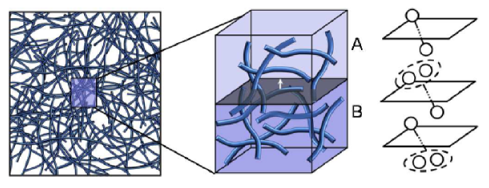
To obtain a notion of macroscopic stress we define a normal direction and a plane which cuts the unit cell. We then determine on average the forces exerted by the particles which lie above this plane on the particles which lie below this plane. We define the effective stress associated with this plane as the total of this exerted force divided by the area of the plane. To define an effective macroscopic stress we average over all possible planes within the unit cell having the specified normal direction, see Figure 5.

Fig. 5: An effective macroscopic stress is estimated from a sample of the material by computing the forces transmitted across a plane which cuts through the sample at a specified location and with a specified normal. At the level of the microstructures, the cut-plane is used to divide the sample into two bodies labeled $A$ and $B$, shown in the middle. The effective stress is estimated by computing the force exerted by particles in body $A$ on particles in body $B$. For models with two body interactions a contribution is made to the stress only if one particle is in body $A$ while the other is in body $B$, shown on the far right on top. For three body interactions there are two possible cases for how forces can be transmitted across the cut plane, shown on the far right in the middle and bottom.

More precisely, the effective macroscopic stress arising from n-body interactions is estimated using

$$\sigma_{\ell,z}^{(n)}=\frac{1}{L}\left\langle\int_{a}^{b}\Lambda_{\ell,z}^{(n)}(\zeta)d\zeta\right\rangle.$$ (55)

The $L=b-a$ is the length of the domain in the $z$-direction and $<\cdot>$ denotes averaging over the ensemble. The $\Lambda_{\ell,z}^{(n)}$ denotes the microscopic stress arising from the $n$-body interactions associated with a given stress plane and is defined by

$$\Lambda_{\ell,z}^{(n)}(\zeta) = \frac{1}{A}\sum_{\mathbf{q}\in\mathcal{Q}_{n}}\sum_{k=1}^{n-1}\sum_{j=1}^{k}\mathbf{f}_{\mathbf{q},j}^{(\ell)}\prod_{j=1}^{k}\mathcal{H}(\zeta-\mathbf{x}_{q_{j}}^{(z)})\prod_{j=k+1}^{n}\mathcal{H}(\mathbf{x}_{q_{j}}^{(z)}-\zeta).$$ (56)

The $\mathcal{Q}_{n}$ is the set of $n$-tuple indices $\mathbf{q}=(q_{1},\ldots,q_{n})$ describing the $n$-body interactions of the system, $\mathbf{f}_{\mathbf{q},j}$ denotes the force acting on the $j^{th}$ particle of the interaction, and $\mathbf{x}_{q_{j}}$ denotes the $j^{th}$ particle involved in the interaction. As a matter of convention in the indexing $\mathbf{q}$ we require that $i\leq j$ implies $\mathbf{x}_{q_{i}}^{(z)}\leq\mathbf{x}_{q_{j}}^{(z)}$. This expression corresponds to a sum over all the forces exerted by particles of the material above the cross-section at $\zeta=z$ on the particles of the material below. Each term of the summation over $k=1,\ldots,n-1$ corresponds to a specific number of particles of the $n$-body interaction lying below the cross-section at $\zeta=z$, see Figure 5.

When integrating the microscopic stress, a useful identity is that

$$\int_{a}^{b}\Pi_{j=1}^{k}\mathcal{H}(\zeta-\mathbf{x}_{q_{j}}^{(z)})\cdot\Pi_{j=k+1}^{n}\mathcal{H}(\mathbf{x}_{q_{j}}^{(z)}-\zeta)d\zeta=\mathbf{x}_{q_{k+1}}^{*,(z)}-\mathbf{x}_{q_{k}}^{*,(z)}$$ (57)

where

$$\mathbf{x}_{q_{j}}^{*,(z)}=\left\{\begin{array}[]{ll}b,&\mbox{if $\mathbf{x}_{q_{j}}^{(z)}\geq b$}\\ \mathbf{x}_{q_{j}}^{(z)},&\mbox{if $a\leq\mathbf{x}_{q_{j}}^{(z)}\leq b$}\\ a,&\mbox{if $\mathbf{x}_{q_{j}}^{(z)}\leq a$}.\\ \end{array}\right.$$ (61)

By integrating equation 56 we obtain

$$\int_{a}^{b}\Lambda_{(\ell),z}^{(n)}(\zeta)d\zeta=\frac{1}{A}\sum_{\mathbf{q}\in\mathcal{Q}_{n}}\sum_{k=1}^{n-1}\sum_{j=1}^{k}\mathbf{f}_{\mathbf{q},j}^{(\ell)}\cdot\left(\mathbf{x}_{q_{k+1}}^{*,(z)}-\mathbf{x}_{q_{k}}^{*,(z)}\right).$$ (62)

This can be further simplified by switching the order of summation of $j$ and $k$ and using the telescoping property of the summation over $k$. From equation 56 this yields the following estimator for the stress contributions of the $n$-body interactions

$$\sigma_{\ell,z}^{(n)}=\frac{1}{AL}\sum_{\mathbf{q}\in\mathcal{Q}_{n}}\sum_{j=1}^{n-1}\left\langle\mathbf{f}_{\mathbf{q},j}^{(\ell)}\cdot\left(\mathbf{x}_{q_{n}}^{*,(z)}-\mathbf{x}_{q_{j}}^{*,(z)}\right)\right\rangle.$$ (63)

This defines an effective macroscopic stress tensor contribution in terms of the n-body interactions of the microstructures of the material. To obtain the total contribution of the microstructure interactions to the stress, all of the contributions of the n-body interactions are summed to obtain the effective macroscopic stress tensor

$$\sigma_{\ell,z}=\sum_{n}\sigma_{\ell,z}^{(n)}.$$ (64)

This notion of the macroscopic stress will be used to link bulk rheological properties to the microscopic simulations.

8.2 Application I: Complex Fluid of Finite Extensible Non-linear Elastic (FENE) Dimers

Fig. 6: Components of the second moment of the extension vector are shown as the shear rate is varied. The second moment matrix is $M=\langle\mathbf{z}\mathbf{z}^{T}\rangle$. On the left is shown the off diagonal entry $M_{1,3}$ as a function of shear rate. On the right is shown the averaged mean squared extension vector of the dimer, which is given by $\bar{\ell}^{2}=\langle|\mathbf{z}|^{2}\rangle=\mbox{Trace}[M]$. The moments show a significant dependence on the rate of shear.

As a demonstration of the proposed computational methodology we consider a fluid with microstructures consisting of elastic polymers. The polymers are modeled as idealized elastic dimers which have the potential energy

$$\phi(r)=\frac{1}{2}Kr_{0}^{2}\log\left(1-\left(\frac{r}{r_{0}}\right)^{2}\right).$$ (65)

The $K$ denotes the polymer stiffness, $r$ denotes the length of extension of the dimer, and $r_{0}$ denotes the maximum permitted extension length [Bird1987Vol2, ]. The configuration of each dimer will be represented using two degrees of freedom $\mathbf{X}^{(1)}$, $\mathbf{X}^{(2)}$. The potential energy for the dimer is given by $\Phi(\mathbf{X})=\phi(|\mathbf{X}^{(2)}-\mathbf{X}^{(1)}|)$, where $\mathbf{X}$ is the composite vector for the particle configuration.

Parameter	Description
$N$	Number of mesh points in each direction.
$\Delta{x}$	Mesh spacing.
$L$	Domain size in each direction.
$T$	Temperature.
$k_{B}$	Boltzmann’s constant.
$\mu$	Dynamic viscosity of the solvent fluid.
$\rho$	Mass density of the solvent fluid.
$K$	Bond stiffness.
$r_{0}$	Maximum permissible bond extension.
$\gamma_{s}$	Stokesian drag of a particle.
$\dot{\gamma}^{0}$	Shear rate amplitude.
$\gamma^{0}$	Strain rate amplitude.
$a$	Effective radius of particle estimated via Stokes drag.

Table 1: Description of the parameters used in simulations of the FENE polymeric fluid.

Parameter	Value
$N$	36
$\Delta{x}$	$11.25\mbox{ nm}$
$L$	$405\mbox{ nm}$
$T$	$300\mbox{ K}$
$k_{B}$	$8.3145\times 10^{3}\mbox{ nm}^{2}\cdot\mbox{amu}\cdot\mbox{ns}^{-2}\cdot\mbox{K}^{-1}$
$\mu$	$6.0221\times 10^{5}\mbox{ amu}\cdot\mbox{cm}^{-1}\cdot\mbox{ns}^{-1}$
$\rho$	$6.0221\times 10^{2}\mbox{ amu}\cdot\mbox{nm}^{-3}$
$K$	$8.9796\times 10^{3}\mbox{ amu}\cdot\mbox{ns}^{-2}$
$r_{0}$	$200\mbox{ nm}$
$\gamma_{s}$	$1.7027\times 10^{8}\mbox{ amu}\cdot\mbox{ns}^{-1}$
$a$	$15\mbox{ nm}$

Table 2: Values of the parameters used in simulations of the FENE polymeric fluid.

When the polymeric fluid is subject to shear the thermally fluctuating polymeric microstructures are expected to significantly re-orient and deform as a consequence of the shear stresses. This along with thermal fluctuations of the microstructures is expected to play an important role in the bulk response of the polymeric fluid. To link the bulk material properties of the fluid to the microstructures, we use the effective macroscopic stress $\sigma_{p}$ obtained from equation 63. To characterize the bulk rheological response we consider the shear viscosity $\eta_{p}$ and first normal stress coefficient $\Psi_{1}$ of the polymeric fluid. We define these as [Bird1987Vol1, ; Bird1987Vol2, ]

$$\eta_{p} = {\sigma_{p}^{(s,v)}}/{\dot{\gamma}}$$ (66)

$$\Psi_{1} = ({\sigma_{p}^{(s,s)}-\sigma^{(v,v)}})/{\dot{\gamma}^{2}}.$$ (67)

The $\dot{\gamma}$ is the rate of shear of the polymeric fluid. In the notation, the superscript $(s,v)$ indicates the tensor component with the index $s$ corresponding to the direction of shear and the index $v$ corresponding to the direction of the fluid velocity. The contributions of the solvent fluid to the shear viscosity and normal stresses can be considered separately [Bird1987Vol2, ].

Fig. 7: Rheological properties of the FENE polymeric fluid are shown as the rate of shear is varied. The shear viscosity is shown on the left and the first normal stress difference is shown on the right. As the shear rate increases the dimers align increasingly with the direction of fluid flow, shown as insets.

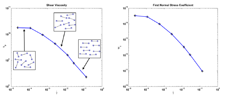
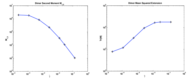
The SELM approach is used to study how the shear viscosity and first normal stress difference depend on the rate of shear of the polymeric fluid. Simulations are performed using the SELM method in the regime where the hydrodynamic modes are relaxed to statistical steady-state with parameters given in Table 1. For $\Lambda$ and $\Gamma$ the coupling tensors of equation 17 and equation 18 are used. From an ensemble average over many computational experiments the moments of the extension vector $\mathbf{z}$ are estimated as the shear rate is increased. The polymeric microstructure moments are seen to respond strongly as the shear stresses of the fluid increase, see Figure 6. This indicates that the rheological properties of the polymeric fluid will depend significantly on the rate of shear. The SELM simulations show that the shear viscosity and the first normal stress difference do in fact vary significantly with the shear rate, see Figure 7.

The shear viscosity is found to decrease as the shear rate increases. This appears to occur as a consequence of the dimers increasingly aligning with the direction of the fluid flow and as a consequence of the dimers approaching the maximal extension permitted by equation 65. The increased extension results in a non-linear increase in the effective stiffness of the dimer (defined for a given extension by Taylor expanding to second order equation 65). While the dimers become increasingly extended with stronger restoring forces this is counter-balanced by the dimers being increasingly stiff and the thermal fluctuations less frequently driving the dimer into configurations crossing the stress plane. The net effect is that the mechanical stress transmitted on average by the dimers in the direction of shear does not increase as the shear rate increases. This results in a lower effective shear viscosity (note the division by $\dot{\gamma}$ in equation 66). This is a well-known phenomena in polymeric fluids and is referred to as shear thinning. The simulations demonstrate that the SELM approach is capable of capturing at the level of the microstructures such phenomena, see Figure 7.

8.3 Application II: Polymerized Lipid Vesicle Fluid

As a further demonstration of the applicability of the SELM approach we show how the stochastic numerical methods can be used to investigate the bulk material properties of a complex fluid with polymerized vesicle microstructures. We discuss how the methods can be used to compute the response of the complex fluid subject to an oscillating shear flow varied over a wide range of frequencies.

Fig. 8: Recursive Method for Mesh Construction. The triangulated mesh for a spherical vesicle is constructed by starting with the vertices and faces of a regular icosahedron, shown on the left. The edges of the icosahedron are bisected and connected to divide each triangular face into four smaller triangular faces. The vertices located at the bisection points are projected radially outward to the surface of the sphere, shown in the middle. This refinement procedure is repeated recursively until a mesh of sufficient resolution is obtained. The mesh obtained after two levels of recursive refinement, which we use to represent polymerized vesicles, is shown on the right.

To obtain a triangulated mesh which captures the shape of a vesicle having a spherical geometry we start with an icosahedral which is circumscribed by a sphere of a given radius. We use the faces of the icosahedron as an initial triangulated mesh. To obtain a mesh which better approximates the sphere we bisect the three edges of each triangular face to obtain four sub-triangles. The newly introduced vertices are projected radially outward to the surface of the sphere. The process is then repeated recursively to obtain further refinements of the mesh. This yields a high quality mesh for spherical geometries. A vesicle represented by a mesh obtained using two levels of recursive refinement is shown in Figure 8.

To account for the mechanics of a polymerized vesicle the following interactions are used for the control points of the mesh

$$\phi_{1}(r,\ell) = \frac{1}{2}K_{1}\left(r-\ell\right)^{2}$$ (68)

$$\phi_{2}(\boldsymbol{\tau}_{1},\boldsymbol{\tau}_{2}) = \frac{1}{2}K_{1}\left|\boldsymbol{\tau}_{1}-\boldsymbol{\tau}_{2}\right|^{2}.$$ (69)

The $r$ denotes the displacement between two control points, $\ell$ denotes a preferred distance between control points, and $\boldsymbol{\tau}$ denotes a normalized displacement vector (tangent vector) between two control points. The $\phi_{1}$ energy accounts for the stretching of a bond between two control points beyond its preferred extension. The $\phi_{2}$ energy accounts for bending of the surface locally by penalizing the misalignment of tangent vectors.

For a given triangulated mesh of control points the total energy is given by

$$\Phi[\mathbf{X}] = E_{1}[\mathbf{X}]+E_{2}[\mathbf{X}]$$ (70)

$$E_{1}[\mathbf{X}] = \sum_{(i,j)\in\mathcal{Q}_{1}}\phi_{1}(r_{ij},\ell_{ij})$$ (71)

$$E_{2}[\mathbf{X}] = \sum_{(i,j,k)\in\mathcal{Q}_{2}}\phi_{2}(\boldsymbol{\tau}_{ij},\boldsymbol{\tau}_{jk}).$$ (72)

The $\mathbf{X}$ denotes the composite vector of control points. The $j^{th}$ control point is denoted by $\mathbf{X}^{[j]}$. The $\mathcal{Q}_{1}$ and $\mathcal{Q}_{2}$ are index sets defined by the topology of the triangulated mesh.

The first energy term $E_{1}$ accounts for stretching of the vesicle surface and is computed by summing over all local two body interactions $\mathcal{Q}_{1}$ defined by the topology of the triangulated mesh. For the distance $r_{ij}=|\mathbf{X}^{[i]}-\mathbf{X}^{[j]}|$ between the two points having index $i$ and $j$, the energy $E_{1}$ penalizes deviations from the preferred distance $\ell_{ij}$. The preferred distances $\ell_{ij}$ are defined by the geometry of a spherical reference configuration for the vesicle. To ensure the two body interactions are represented by a unique index in $\mathcal{Q}_{1}$ we adopt the convention that $i<j$.

The second energy term $E_{2}$ accounts for curvature of the vesicle surface and is computed by summing over all local three body interactions $\mathcal{Q}_{2}$ defined by the topology of the triangulated mesh. The energy penalizes the the misalignment of the tangent vectors $\boldsymbol{\tau}_{ij}=(\mathbf{X}^{[i]}-\mathbf{X}^{[j]})/r_{ij}$ and $\boldsymbol{\tau}_{jk}=(\mathbf{X}^{[j]}-\mathbf{X}^{[k]})/r_{jk}$. In the set of indices in $\mathcal{Q}_{2}$ it is assumed that the point with index $j$ is always adjacent to both $i$ and $k$. To ensure the three body interactions are represented by a unique index in $\mathcal{Q}_{2}$ we adopt the convention that $i<k$.

Fig. 9: Simulation results showing the vesicle response when subject to an oscillating shear flow. At low frequency the vesicle shape distortion is small and is masked by thermal fluctuations. At low frequency the vesicle membrane stresses equilibrate to a good approximation with the bulk shear stresses, as illustrated in the plot of $\sigma_{xz}$ . For the vesicle configurations shown, the low frequency response corresponds to $\omega=3.9294\times 10^{-3}\mbox{ns}^{-1}$, $\dot{\gamma}=1.9647\times 10^{-3}\mbox{ns}^{-1}$, $\sigma_{0}=3.7114\times 10^{8}\mbox{amu}\cdot\mbox{nm}^{-1}\cdot\mbox{ns}^{-2}$. The phase $\theta=\omega{t}$ is reported in the range $[0,2\pi)$. For additional parameters used in the simulations see Table 3 and 4.

Fig. 10: Simulations results showing the vesicle response when subject to an oscillating shear flow. At high frequency the vesicle shape is visibly distorted and the membrane stresses do not have time to equilibrate with the bulk shear stresses, as illustrated by the configurations for phase $\theta=1.6,0.4$ and the plot of $\sigma_{xz}$. For the vesicle configurations shown, the high frequency response corresponds to $\omega=1.2426\times 10^{2}\mbox{ns}^{-1}$, $\dot{\gamma}=6.2129\times 10^{1}\mbox{ns}^{-1}$, $\sigma_{0}=4.6314\times 10^{10}\mbox{amu}\cdot\mbox{nm}^{-1}\cdot\mbox{ns}^{-2}$. The phase $\theta=\omega{t}$ is reported in the range $[0,2\pi)$. For additional parameters used in the simulations see Table 3 and 4.

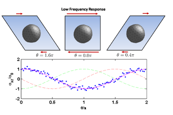
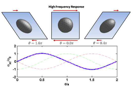
To investigate the bulk rheological properties, the complex vesicle fluid is subjected to an oscillatory shear with rate $\dot{\gamma}=\dot{\gamma}^{0}\cos(\omega t)$. We consider the dilute regime in which it is sufficient to study a single polymerized vesicle subject to oscillatory shear. To estimate the effective macroscopic stress tensor the tensor is decomposed into contributions from two body and three body interactions

$$\sigma_{\ell,z}=\sigma_{\ell,z}^{(2)}+\sigma_{\ell,z}^{(3)}.$$ (73)

For the contributions of the n-body interactions to the macroscopic stress $\sigma_{\ell,z}^{(n)}$ we use the approach discussed in Section 8.1 and the specific estimator given by equation 63.

For many materials, the responses of the stress component $\sigma_{xz}(t)$ to bulk stresses and strains are linear to a good approximation over a wide range of frequencies provided the stress and strain amplitudes are sufficiently small [bird1987, ]. As a measure of the material response, we consider the dynamic complex modulus $G(\omega)=G^{\prime}(\omega)+iG^{\prime\prime}(\omega)$, whose components are defined from measurements of the stress as the best least-squares fit of the periodic stress component $\sigma_{xz}(t)$ by the function $g(t)=G^{\prime}(\omega)\gamma^{0}\cos(\omega t)+G^{\prime\prime}(\omega)\gamma^{0}\sin(\omega t)$. This offers one characterization of the response of the material to oscillating bulk shear stresses and strains as the frequency $\omega$ is varied.

To estimate the dynamic complex modulus in practice the least squares fit is performed for $\sigma_{xz}(t)$ over the entire stochastic trajectory of the simulations (after some transient period). Throughout our discussion we refer to $\theta=\omega{t}$ as the phase of the periodic response. In our simulations the maximum strain each period was chosen to always be half the periodic unit cell in the x-direction, corresponding to strain amplitude $\gamma^{0}=\frac{1}{2}$. This was achieved by adjusting the shear rate amplitude for each frequency using $\dot{\gamma}^{0}=\gamma^{0}\omega$.

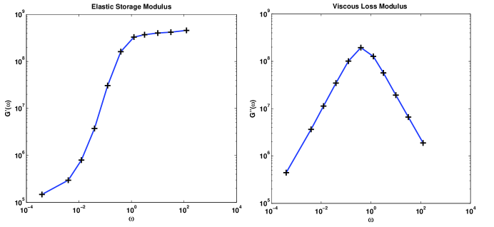
Simulations were performed with the SELM approach in the regime where the hydrodynamic modes were treated as relaxed to statistical steady-state. The specific coupling operators $\Lambda$ and $\Gamma$ from 17 and 18 were used. The simulation results of the complex modulus response of the vesicle when subject to a wide range of frequencies is shown in Figure 9, Figure 10, and Figure 11. It was found that at low frequency the vesicle shape distortion is small and masked by thermal fluctuations. At low frequency the vesicle membrane stresses equilibrate to a good approximation with the bulk shear stresses, as illustrated in the plot of $\sigma_{xz}$ in Figure 9. It was found at high frequency the vesicle shape is visibly distorted and the membrane stresses do not have time to equilibrate with the bulk shear stresses, as illustrated by the configurations for phase $\theta=1.6,0.4$ and the plot of $\sigma_{xz}$ in Figure 10. For the vesicle configurations shown, the low frequency response corresponds to $\omega=3.9294\times 10^{-3}\mbox{ns}^{-1}$, $\dot{\gamma}=1.9647\times 10^{-3}\mbox{ns}^{-1}$, $\sigma_{0}=3.7114\times 10^{8}\mbox{amu}\cdot\mbox{nm}^{-1}\cdot\mbox{ns}^{-2}$, and the high frequency response corresponds to $\omega=1.2426\times 10^{2}\mbox{ns}^{-1}$, $\dot{\gamma}=6.2129\times 10^{1}\mbox{ns}^{-1}$, $\sigma_{0}=4.6314\times 10^{10}\mbox{amu}\cdot\mbox{nm}^{-1}\cdot\mbox{ns}^{-2}$. The phase $\theta=\omega{t}$ is reported in the range $[0,2\pi)$. A description of the parameters and specific values used in the simulations can be found in Table 3 and 4.

Fig. 11: Frequency response of the dynamic complex modulus of the vesicle fluid subject to an oscillating shear flow. Throughout the simulations the total strain was held fixed to be half the domain length, $\gamma^{0}=\frac{1}{2}L$. For a description of the parameters and values used in the simulations, see Table 3 and 4.

Parameter	Description
$N$	Number of mesh points in each direction.
$\Delta{x}$	Mesh spacing.
$L$	Domain size in each direction.
$T$	Temperature.
$k_{B}$	Boltzmann’s constant.
$\mu$	Dynamic viscosity of the solvent fluid.
$\rho$	Mass density of the solvent fluid.
$K_{1}$	Vesicle bond stiffness.
$K_{2}$	Vesicle bending stiffness.
$D$	Vesicle diameter.
$\omega$	Frequency of oscillating shearing motion.
$\theta$	Phase of the oscillatory motion, $\theta=\omega t$.
$\dot{\gamma}$	Shear rate.
$\dot{\gamma}^{0}$	Shear rate amplitude.
$\gamma$	Strain rate.
$\gamma^{0}$	Strain rate amplitude.

Table 3: Description of the parameters used in simulations of the vesicle fluid.

Parameter	Value
$N$	$27$
$\Delta{x}$	$7.5\mbox{ nm}$
$L$	$2.025\times 10^{2}\mbox{ nm}$
$T$	$300\mbox{ K}$
$k_{B}$	$8.3145\times 10^{3}\mbox{ nm}^{2}\cdot\mbox{amu}\cdot\mbox{ns}^{-2}\cdot\mbox{K}^{-1}$
$\mu$	$6.0221\times 10^{5}\mbox{ amu}\cdot\mbox{cm}^{-1}\cdot\mbox{ns}^{-1}$
$\rho$	$6.0221\times 10^{2}\mbox{ amu}\cdot\mbox{nm}^{-3}$
$\mbox{K}_{1}$	$2.2449\times 10^{7}\mbox{ amu}\cdot\mbox{ns}^{-2}$
$\mbox{K}_{2}$	$8.9796\times 10^{7}$
$D$	$50\mbox{ nm}$

Table 4: Fixed values of the parameters used in simulations of the vesicle fluid.

8.4 Application III: Rheology of a Gel-like Material

As a further demonstration of the applicability of the SELM approach we show how the stochastic numerical methods can be used to investigate properties of a gel-like material subject to shear. The methods are used to study how the shear viscosity changes over time as the gel is subjected to shear at a constant rate.

Fig. 12: Model for a Gel-Like Material. The gel is formed by polymeric chains which bind together, shown on the left. The polymeric chains are each comprised of five control points and have specialized binding sites at the second and fourth control point, shown in the center. The inter-polymer bonds have a preferred extension and angle. When an inter-polymer bond is strained beyond $50\%$ of its preferred rest length the bond breaks irreversibly, shown on the right.

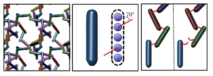
The gel-like material is modeled as a collection of polymer chains which are able to bond together at two specialized sites along the chain, see Figure 12. The energy associated with the mechanics of the individual polymer chains and the bonds which they form are given by

$$\phi_{1}(r) = \frac{1}{2}K_{1}(r-r_{0,1})^{2}$$ (74)

$$\phi_{2}(\boldsymbol{\tau}_{1},\boldsymbol{\tau}_{2}) = \frac{1}{2}K_{2}\left|\boldsymbol{\tau}_{1}-\boldsymbol{\tau}_{2}\right|^{2}$$ (75)

$$\phi_{3}(r) = \sigma^{2}K_{3}\exp\left[-\frac{(r-r_{0,3})^{2}}{2\sigma^{2}}\right]$$ (76)

$$\phi_{4}(\theta) = -K_{4}\cos(\theta-\theta_{0,4}).$$ (77)

The $r$ is the separation distance between two control points, $\theta$ is the bond angle between three control points, and $\boldsymbol{\tau}$ is a tangent vector along the polymer chain, see Figure  12.

The $\phi_{1}$ energy accounts for stretching of a bond within a polymer chain from its preferred extension $r_{0,1}$. The $\phi_{2}$ energy accounts for bending of the polymer chain locally. To account for interactions at the specialized binding sites of the polymers the potentials $\phi_{3}$ and $\phi_{4}$ are introduced. The potential $\phi_{3}$ gives the energy of the bond between the two polymer chains and penalizes deviation from the preferred bond extension $r_{0,3}$. The exponential of $\phi_{3}$ is introduced so that the resistance in the bond behaves initially like a harmonic bond but decays rapidly to zero when the bond is stretched beyond the length $\sigma$. The potential $\phi_{4}$ gives the energy for the preferred bond angle when two of the polymer chains are bound together.

The total energy of the system is given by

$$\Phi[\mathbf{X}] = E_{1}[\mathbf{X}]+E_{2}[\mathbf{X}]+E_{3}[\mathbf{X}]+E_{4}[\mathbf{X}]$$ (78)

$$E_{1}[\mathbf{X}] = \sum_{(i,j)\in\mathcal{Q}_{1}}\phi_{1}(r_{ij}),\mbox{\hskip 7.11317pt}E_{2}[\mathbf{X}]=\sum_{(i,j,k)\in\mathcal{Q}_{2}}\phi_{2}(\boldsymbol{\tau}_{ij},\boldsymbol{\tau}_{jk})$$ (79)

$$E_{3}[\mathbf{X}] = \sum_{(i,j)\in\mathcal{Q}_{3}}\phi_{3}(r_{ij}),\mbox{\hskip 7.11317pt}E_{4}[\mathbf{X}]=\sum_{(i,j,k)\in\mathcal{Q}_{4}}\phi_{4}(\theta_{ijk}).$$ (80)

The sets $\mathcal{Q}_{k}$ define the interactions according to the structure of the individual polymer chains and the topology of the gel network. When bonds are stretched beyond the critical length $3\sigma$ they are broken irreversibly, which results in the sets $\mathcal{Q}_{3}$ and $\mathcal{Q}_{4}$ being time dependent.

Fig. 13: Study of the shear viscosity of a gel-like material. At time zero the material has weak bonds between short polymeric chains. Under the shear deformation the gel is stretched and the bonds are strained until ultimately breaking. Many of the polymers are misaligned with the direction of fluid flow and are further stretched by the fluid shear stresses. As the polymer chains align with the direction of fluid flow the forces transmitted in the direction of shear decrease and the shear viscosity approaches a steady-state value. The thermal fluctuations maintain transient misalignments of the polymer chains which transmit forces in the direction of shear resulting in a contribution to the shear viscosity which is non-zero at steady-state. The microstructure reordering in each of these stages, labeled I, II, III, is reflected in the shear viscosity of the material as a function of time and in Figure 14. For the specific physical parameters used in these simulation see Table 5 and 6.

Fig. 14: The microstructure of a gel-like material at three different times. On the left is shown the microstructure of the gel-like material before any shear has been applied. In the middle is show the microstructure of the gel after almost all of the bonds between polymer chains have been broken. In this case, the misaligned polymer chains continue to be stretched by the shear stresses of the fluid yielding a relatively large effective shear viscosity. On the right is shown the microstructure of the gel when the system has relaxed to statistical steady-state. In this case, the thermal fluctuations drive transient misalignments of the polymer chains with the direction of flow which on average make a non-zero contribution to the shear viscosity. The times shown in each of these figures is $t=0\mbox{ ns}$, $t=2844\mbox{ ns}$, $t=7111\mbox{ ns}$. For the specific physical parameters used in these simulations see Table 5 and 6.

Parameter	Description
$N$	Number of mesh points in each direction.
$\Delta{x}$	Mesh spacing.
$\Delta{t}$	Time step.
$L$	Domain size in each direction.
$T$	Temperature.
$k_{B}$	Boltzmann’s constant.
$\mu$	Dynamic viscosity of the solvent fluid.
$\rho$	Mass density of the solvent fluid.
$\dot{\gamma}$	Shear rate.
$N_{p}$	Number of polymer chains.
$N_{s}$	Number of control points per polymer chain.
$r_{p}$	Polymer effective cylindrical radius.
$K_{1}$	Stiffness of the bonds of the polymer chain.
$r_{0,1}$	Rest length of the bonds of the polymer chain.
$K_{2}$	Bending stiffness of the polymer chain.
$K_{3}$	Stiffness of the bonds at a polymer binding site.
$r_{0,3}$	Rest length of the bond at a polymer binding site.
$K_{4}$	Bending stiffness of the bond at a polymer binding site.
$\theta_{0,4}$	Preferred angle of a bond at a polymer binding site.

Table 5: Description of the parameters used in simulations of the gel-like material.

Parameter	Value
$N$	$72$
$\Delta{x}$	$11.25\mbox{ nm}$
$\Delta{t}$	$1.4222\mbox{ ns}$
$L$	$810\mbox{ nm}$
$T$	$300\mbox{ K}$
$k_{B}$	$8.3145\times 10^{3}\mbox{ nm}^{2}\cdot\mbox{amu}\cdot\mbox{ns}^{-2}\cdot\mbox{K}^{-1}$
$\mu$	$6.0221\times 10^{5}\mbox{ amu}\cdot\mbox{cm}^{-1}\cdot\mbox{ns}^{-1}$
$\rho$	$6.0221\times 10^{2}\mbox{ amu}\cdot\mbox{nm}^{-3}$
$\dot{\gamma}$	$1.2\times 10^{-3}\mbox{ ns}^{-1}$
$N_{p}$	$110$
$N_{s}$	$5$
$r_{p}$	$15\mbox{ nm}$
$K_{1}$	$2.9932\times 10^{5}\mbox{ amu}\cdot\mbox{ns}^{-2}$
$r_{0,1}$	$30\mbox{ nm}$
$K_{2}$	$2.9932\times 10^{8}$
$K_{3}$	$2.9932\times 10^{5}\mbox{ amu}\cdot\mbox{ns}^{-2}$
$r_{0,3}$	$30\mbox{ nm}$
$K_{4}$	$2.9932\times 10^{8}$
$\theta_{0,4}$	$70\,^{\circ}$

Table 6: Fixed values of the parameters used in simulations of the gel-like material.

To study the rheological response of the gel-like material the system is subjected to shear at a constant rate. To obtain an effective macroscopic stress $\sigma_{p}$ for the system the estimator is used from equation 63. To characterize the rheological response we use the shear viscosity defined by

$$\eta_{p} = {\sigma_{p}^{(s,v)}}/{\dot{\gamma}}.$$ (81)

The $\dot{\gamma}$ is the rate of shear of the polymeric fluid. In the notation, the superscript $(s,v)$ indicates the tensor component with the index $s$ corresponding to the direction of shear and the index $v$ corresponding to the direction of the fluid velocity. The contributions of the solvent fluid to the shear viscosity can be considered separately [Bird1987Vol2, ].

The entire gel network experiences an unbounded shear deformation. This is expected to result in breakage of bonds of the gel network. This suggests that the rheological response will depend on how long the material has been subject to shear. To investigate the role reorganization at the microstructure level, repeated stochastic simulations are carried out using the SELM approach to determine the effective shear viscosity of the material as a function of time.

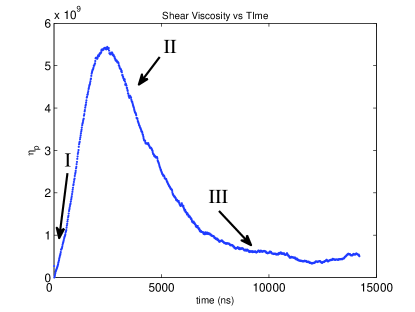
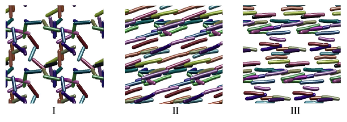
An interesting behavior is found in which the material initially exhibits an increased shear viscosity before settling down to a steady-state value. The responses of the material to shear can be roughly divided into three stages. In the first, there is an initial increase which can be attributed to the stretching of the inter-chain bonds between the polymer chains and the intra-chain bonds within each polymer chain, which occurs as the gel as a whole is strained. After a relatively short period, the bonds between the polymer chains are observed to break with the remaining stress arising from the stretching of the polymer chains which occurs from the shear stresses of the fluid and misalignment with the direction of flow, see the region labeled by I in Figure 13 and 14.

In the second stage, the individual polymer chains rotate and begin to align with the direction of flow. As a result of the intra-chain restoring forces the strain of the individual polymer chains is reduced. The increased alignment and reduced strain of the polymer chains yields an overall decrease in the forces transmitted in the direction of shear. Consequently, the shear viscosity begins to decrease, see the region labeled by II in Figure 13 and 14.

In the last stage, the chains eventually settle into a statistical steady-state in which the thermal fluctuations drive the chains to misalign only transiently with the flow direction. These misaligned excursions by the polymer chains sustained by the thermal fluctuations result in forces transmitted in the direction of shear on average. This is reflected in the shear viscosity by a non-zero steady-state value, see the region labeled by III in Figure 13 and 14.

Using the SELM approach more complicated situations could also be studied, such as the case in which the bonds between the polymer chains are able to reform. An interesting investigation in this case would be to study how the viscosity behaves after decreasing or ceasing shearing of the system for a period of time. In this case the gel would have time to reform structures before being again subjected to large shears. Using such a SELM approach a widely variety of shear thinning and thixotropic phenomena could be studied at the level of the microstructures [Barnes1997, ; Bird1987Vol2, ; Doi1986, ].

9 Conclusions

A general formalism was developed which allows for the coupling of Eulerian and Lagrangian descriptions of physical systems. A general approach was introduced for incorporating thermal fluctuations in such descriptions. The approach addresses both the inertial regime and the overdamped regime. For the study of rheological responses of materials, an approach was developed which allows for generalized periodic boundary conditions which induce the shear. For simulations using the formalism stochastic numerical methods were developed which efficiently generate the required stochastic driving fields. As a demonstration of how these methods can be used in practice, simulation studies were carried out for complex fluids and soft materials. The basic Stochastic Eulerian Lagrangian Method (SELM) approach is expected to be useful in the formulation of descriptions and computational approaches for the study of a wide variety of fluid structure phenomena involving thermal fluctuations.

10 Acknowledgements

The author P.J.A. acknowledges support from research grant NSF DMS-0635535. We would especially like to thank Aleksandar Donev, Alejandro Garcia, John Bell, and Tony Ladd for stimulating conversations about this work. This paper is dedicated in memorial to Tom Bringley, whose academic publications continue to inspire. His passion for life, mathematics, and science will be greatly missed.

Appendix A Invariance of the Boltzmann Distribution under SELM Stochastic Dynamics

The probability distribution of the stochastic equations 1-2 are governed formally by the Fokker-Planck equation

$$\frac{\partial\Psi}{\partial t}=-\nabla\cdot\mathbf{J}$$ (82)

with the probability flux given by

$$\mathbf{J} = \left[\begin{array}[]{l}\mathcal{L}\mathbf{p}\Psi+(\Lambda+\lambda)\Psi-\frac{1}{2}G\nabla_{\mathbf{p}}\Psi\\ (\Gamma+\gamma)\Psi-\frac{1}{2}W\nabla_{\mathbf{X}}\Psi\end{array}\right].$$ (85)

The $G$, $W$ are the covariance operators associated with $\mathbf{g}$ and $\mathbf{Z}$. The $\Psi(\mathbf{p},\mathbf{X},t)$ is the formal probability density for finding the system in state $(\mathbf{p},\mathbf{X})$ at time $t$. For the present purposes our discussion will only be formal since the SPDEs are infinite dimensional and for the density there is no Lebesgue measure for the function space, see [Oksendal2000, ; Gardiner1985, ; Da1992, ]. In practice a finite dimensional stochastic process will always be used to approximate the SPDEs and has a probability distribution satisfying a well-defined equation.

For the systems under consideration, the Boltzmann distribution has the form $\Psi_{BD}(\mathbf{p},\mathbf{X})=\frac{1}{Z}\exp\left[-{E[\mathbf{p},\mathbf{X}]}/{k_{B}T}\right]$, where $Z$ is a normalization constant so that $\Psi_{BD}$ integrates to one [Reichl1998, ]. The requirement that this distribution is invariant under the stochastic dynamics of 1-2 is equivalent to $\nabla\cdot\mathbf{J}=0$. This requires

$$\nabla\cdot\mathbf{J} = A_{1}+A_{2}+\nabla\cdot\mathbf{A}_{3}=0$$ (86)

$$A_{1} = \left[(\Lambda+\lambda)\cdot\nabla_{\mathbf{p}}E+(\Gamma+\gamma)\cdot\nabla_{\mathbf{X}}E\right](-k_{B}{T})^{-1}\Psi$$ (87)

$$A_{2} = \left(\nabla_{\mathbf{p}}\cdot(\Lambda+\lambda)+\nabla_{\mathbf{X}}\cdot(\Gamma+\gamma)\right)\Psi$$ (88)

$$\mathbf{A}_{3} = \left(\mathcal{L}\mathbf{p}+\frac{G\nabla_{\mathbf{p}}E+W\nabla_{\mathbf{X}}E}{2k_{B}{T}}\right)\Psi.$$ (89)

For the energy given by equation 3 we have

$$\nabla_{\mathbf{p}}E = \rho_{0}^{-1}\mathbf{p}$$ (90)

$$\nabla_{\mathbf{X}}E = \nabla_{\mathbf{X}}\Phi=-\mathbf{F}$$ (91)

where $\mathbf{F}$ denotes the force for the configuration.

Now we can derive conditions for the coupling operators by requiring that $A_{1}=A_{2}=0$ for all possible values of $\mathbf{p}$ and $\mathbf{F}$. The requirement that $A_{1}=0$ corresponds to the energy being conserved under the dynamics of equations 1-2 when $\mathbf{g}=\mathbf{Z}=0$ and $\boldsymbol{\sigma}=0$. For these dynamics the energy satisfies ${dE}/{dt}=(\Lambda+\lambda)\cdot\nabla_{\mathbf{p}}E+(\Gamma+\gamma)\cdot\nabla_{\mathbf{X}}E=0$. Since the forces associated with time independent constraints do not do any work on the system we have that $\lambda\cdot\nabla_{\mathbf{p}}E+\gamma\cdot\nabla_{\mathbf{X}}E=0$. Conservation of energy then requires $\Lambda\cdot\nabla_{\mathbf{p}}E+\Gamma\cdot\nabla_{\mathbf{X}}E=0$. By using the variational derivatives [Gelfand2000, ] of $E$ given in 90-91 we have $\Lambda\cdot\nabla_{\mathbf{p}}E=\int\Lambda\rho_{0}^{-1}\mathbf{p}d\mathbf{x}$ and $\Gamma\cdot\nabla_{\mathbf{X}}E=\int-\Gamma\mathbf{F}d\mathbf{q}$. By substituting these expressions into 87, we obtain from $A_{1}=0$ that the condition 4 must be satisfied.

The requirement that $A_{2}=0$ requires that the dynamical flow in phase space defined by $(\Lambda+\lambda,\Gamma+\gamma)$ is volume preserving. For the dynamics when $\mathbf{g}=\mathbf{Z}=0$, $\boldsymbol{\sigma}=0$, and $E=0$ this condition is equivalent to requiring that the uniform distribution is invariant under the dynamics. The condition 6 follows by using the function representing the variational derivatives [Gelfand2000, ] appearing in the divergence operation corresponds to $\nabla_{\mathbf{X}}\cdot\Gamma=\int(\delta\Gamma/\delta\mathbf{X})(\mathbf{q},\mathbf{q})d\mathbf{q}$, $\nabla_{\mathbf{X}}\cdot\gamma=\int(\delta\gamma/\delta\mathbf{X})(\mathbf{q},\mathbf{q})d\mathbf{q}$, and similarly for $\Lambda$, $\lambda$.

The requirement that $A_{3}=0$ requires from equation 90-91 that
$\mathcal{L}\mathbf{p}+\left[{(G\rho^{-1}\mathbf{p}-W\mathbf{F})}/{2k_{B}{T}}\right]=0$ for any $\mathbf{p}$ and $\mathbf{F}$. This requirement corresponds to the condition of Detailed-Balance of statistical mechanics [Reichl1998, ]. Since $\mathbf{p}$ and $\mathbf{F}$ are arbitrary, this requires that $W=0$ so that $\mathbf{Z}=0$. This also requires that $G=-2\mathcal{L}\mathcal{C}$ with $\mathcal{C}=k_{B}{T}\rho_{0}\mathcal{I}$, where $\mathcal{I}$ is the identity operator. This yields condition 7. From the form of the energy in 3 and the Boltzmann distribution we see the equilibrium fluctuations of $\mathbf{p}$ are Gaussian with covariance $\mathcal{C}$. This condition relates the equilibrium fluctuations to the dissipative operator of the system and is a variant of the Fluctuation-Dissipation Principle of statistical mechanics [Reichl1998, ]. This shows that provided the coupling operators and stochastic fields satisfy conditions 4, 6, and 7, the Boltzmann distribution is invariant under the SELM stochastic dynamics.

For the discretized equations, we now derive conditions 11, 13, and 15. The calculations follow similarly to the case above so we only state the basic features of the derivation. For the discretized equations the probability flux is given by

$$\mathbf{J} = \left[\begin{array}[]{l}L\mathbf{p}\Psi+(\Lambda+\lambda)\Psi-\frac{1}{2}G\nabla_{\mathbf{p}}\Psi\\ (\Gamma+\gamma)\Psi\end{array}\right]$$ (94)

where $\mathbf{p}$ and $\mathbf{X}$ are now finite dimensional vectors. The Boltzmann distribution now uses the energy of the discrete system

$$E[\mathbf{p},\mathbf{X}]=\sum_{\mathbf{m}}\frac{1}{2}\rho_{0}^{-1}|\mathbf{p}_{\mathbf{m}}|^{2}\Delta{x}^{d}+\Phi(\mathbf{X})$$ (95)

with

$$\nabla_{\mathbf{p}}E = \rho_{0}^{-1}\mathbf{p}\Delta{x}^{d}$$ (96)

$$\nabla_{\mathbf{X}}E = \nabla_{\mathbf{X}}\Phi=-\mathbf{F}.$$ (97)

Substituting these expressions in 86 - 89 and reasoning as above yields the conditions 11, 13, and 15.

Appendix B A Fluctuation-Dissipation Principle for Time-Dependent Operators

Consider the stochastic process given by

$$d\mathbf{z}_{t} = L(t)\mathbf{z}dt+Q(t)d\mathbf{B}_{t}$$ (98)

$$G(t) = QQ^{T}.$$ (99)

We now establish the following fluctuation-dissipation relation

$$G(t)=-L(t)\bar{C}-\bar{C}^{T}L(t)^{T}.$$ (100)

This relates the covariance $G(t)$ of the stochastic driving field to a time-dependent dissipative operator $L(t)$ and a time-independent equilibrium covariance $\bar{C}$. We show that this relation allows for $G(t)$ to be chosen to ensure that the stochastic dynamics exhibits at statistical steady-state equilibrium fluctuations with the specified covariance $\bar{C}$.

Let the covariance at time $t$ be denoted by

$$C(t)=\langle\mathbf{u}(t)\mathbf{u}(t)^{T}\rangle.$$ (101)

By Ito’s Lemma the second moment satisfies

$$dC(t)=\left(L(t)C(t)+C(t)^{T}L(t)^{T}+G(t)\right)dt.$$ (102)

It will be convenient to express this equation by considering all of the individual entries of the matrix $C(t)$ collected into a single column vector denoted by $\mathbf{c}_{t}$. Similarly, for covariance matrix $G(t)$ we denote the column vector of entries by $\mathbf{g}_{t}$ and for $\bar{C}$ by $\bar{\mathbf{c}}$. Since the products $L(t)C(t)$ and $C(t)^{T}L(t)^{T}$ are both linear operations in the entries of the matrix $C(t)$ we can express this in terms of multiplication by of a matrix $A(t)$ acting on $\mathbf{c}_{t}$.

This notation allows for equation 102 to be expressed equivalently as

$$d\mathbf{c}_{t}=\left(A(t)\mathbf{c}_{t}+\mathbf{g}_{t}\right)dt.$$ (103)

The equation 102 can be solved formally by the method of integrating factors to obtain

$$\mathbf{c}_{t}=e^{\Xi(0,t)}\mathbf{c}_{0}+\int_{0}^{t}e^{\Xi(s,t)}\mathbf{g}_{s}ds$$ (104)

where $\Xi(s,t)=\int_{s}^{t}A(r)dr$.

The fluctuation-dissipation relation given by equation 100 is equivalent to choosing

$$\mathbf{g}_{s}=-A(s)\bar{\mathbf{c}}.$$ (105)

For this choice, a useful identity is

$$e^{\Xi(s,t)}\mathbf{g}_{s}=\frac{\partial}{\partial s}e^{\Xi(s,t)}\bar{\mathbf{c}}.$$ (106)

Substitution into equation 104 gives

$$\mathbf{c}_{t}=e^{\Xi(0,t)}\mathbf{c}_{0}+\left(e^{\Xi(t,t)}-e^{\Xi(0,t)}\right)\bar{\mathbf{c}}.$$ (107)

Now, if $L(t)$ is negative definite uniformly in time, $\mathbf{v}^{T}L(t)\mathbf{v}<\alpha_{0}<0$, then $A(t)$ is also uniformly negative definite. This implies that

$$\lim_{t\rightarrow\infty}e^{\Xi(0,t)}=0.$$ (108)

Taking the limit of both sides of equation 107 and using equation 108 yields

$$\lim_{t\rightarrow\infty}\mathbf{c}_{t}=\mathbf{\bar{c}}.$$ (109)

This shows that the stochastic driving field with covariance given by equation 100 yields equilibrium fluctuations with covariance $\bar{C}$. This extends the fluctuation-dissipation relation to the case of time-dependent operators.

For the discretization given in Section 4, we point out some of the properties of the specific matrix $L(t)$ which are used. From equation 31 the non-zero eigenvalues of $L(t)$ can be shown to be negative and uniformly bounded away from zero in time. The eigenvector associated with the zero eigenvalue of $L(t)$ is in fact the same for all times. The eigenvector of the zero eigenvalue is proportional to the vector with all components set to one. In practice, this mode is set to zero. By conservation of momentum of the fluid body as a whole, this mode remains zero when subject to internal conservative forces. This allows for the operator $L(t)$ to be considered as acting on the linear space which excludes this null eigenvector. On this linear space, $L(t)$ is strictly negative definite uniformly in time. Similar considerations can be made when considering the effect of the incompressibility constraint for the operator $\tilde{L}(t)=\wp L(t)$. Thus the time-dependent fluctuation-dissipation relation given by equation 100 still holds provided the stochastic process is considered on the appropriate linear space which excludes the null eigenvectors.

Appendix C The Particle Representation Function $\delta_{a}$

In the immersed boundary method, it is required that a function $\delta_{a}$ be specified to represent the elementary particles. The representation of this function is often derived from the following function $\phi$ which is known to have desirable numerical properties  [Peskin2002, ; Atzberger2007a, ]:

$$\phi(r) = \left\{\begin{array}[]{ll}0&\mbox{, if $r\leq-2$}\\ &\\ \frac{1}{8}\left(5+2r-\sqrt{-7-12r-4r^{2}}\right)&\mbox{, if $-2\leq r\leq-1$}\\ &\\ \frac{1}{8}\left(3+2r+\sqrt{1-4r-4r^{2}}\right)&\mbox{, if $-1\leq r\leq 0$}\\ &\\ \frac{1}{8}\left(3-2r+\sqrt{1+4r-4r^{2}}\right)&\mbox{, if $0\leq r\leq 1$}\\ &\\ \frac{1}{8}\left(5-2r-\sqrt{-7+12r-4r^{2}}\right)&\mbox{, if $1\leq r\leq 2$}\\ &\\ 0&\mbox{, if $2\leq r$.}\\ \end{array}\right.$$ (121)

For three dimensional systems the function $\delta_{a}$ representing elementary particles of size $a$ is

$$\delta_{a}(\mathbf{r})=\frac{1}{a^{3}}\phi\left(\frac{\mathbf{r}^{(1)}}{a}\right)\phi\left(\frac{\mathbf{r}^{(2)}}{a}\right)\phi\left(\frac{\mathbf{r}^{(3)}}{a}\right),$$ (122)

where the superscript indicates the index of the vector component.

To maintain good numerical properties, the particles are restricted to sizes $a=n\Delta{x}$, where $n$ is a positive integer. For a derivation and a detailed discussion of the properties of these functions see [Peskin2002, ; Atzberger2007a, ].

Appendix D Table

Parameter	Description
$N_{A}$	Avogadro’s number.
amu	Atomic mass unit.
nm	Nanometer.
ns	Nanosecond.
$k_{B}$	Boltzmann’s Constant.
$T$	Temperature.
$\eta$	Dynamic viscosity of water.
$\gamma_{s}=6\pi\eta R$	Stokes’ drag of a spherical particle.

Parameter	Value
$N_{A}$	$6.02214199\times 10^{23}$.
amu	$1/10^{3}N_{A}$ kg.
nm	$10^{-9}\hskip 2.84544pt\mbox{m}$.
ns	$10^{-9}\hskip 2.84544pt\mbox{s}$.
$k_{B}$	$8.31447\times 10^{3}\hskip 2.84544pt\mbox{amu}\hskip 2.84544pt\mbox{nm}^{2}/\mbox{ns}^{2}\hskip 2.84544ptK$.
$T$	$300\mbox{K}$.
$\eta$	$6.02214199\hskip 2.84544pt\mbox{amu}/\mbox{cm}\hskip 2.84544pt\mbox{ns}$.

References

- [1] P. J. Atzberger, A note on the correspondence of an immersed boundary method incorporating thermal fluctuations with stokesian-brownian dynamics, Physica D-Nonlinear Phenomena, 226 (2007), pp. 144–150–.
- [2] P. J. Atzberger and P. R. Kramer, Error analysis of a stochastic immersed boundary method incorporating thermal fluctuations, Mathematics and Computers in Simulation, 79 (2008), pp. 379–408–.
- [3] P. J. Atzberger, P. R. Kramer, and C. S. Peskin, A stochastic immersed boundary method for fluid-structure dynamics at microscopic length scales, Journal of Computational Physics, 224 (2007), pp. 1255–1292–.
- [4] H. A. Barnes, Thixotropy - a review, Journal of Non-Newtonian Fluid Mechanics, 70 (1997), pp. 1–33–.
- [5] Curtiss C. F. Armstrong R. C. Hassager O. Bird, R.B., Dynamics of Polymeric Liquids : Volume I Fluid Mechanics, Wiley-Interscience, 1987.
- [6] , Dynamics of Polymeric Liquids : Volume II Kinetic Theory, Wiley-Interscience, 1987.
- [7] J. F. Brady and G. Bossis, Stokesian dynamics, Annual review of fluid mechanics. Vol.20—Annual review of fluid mechanics. Vol.20, (1988), pp. 111–57.
- [8] T. T. Bringley and C. S. Peskin, Validation of a simple method for representing spheres and slender bodies in an immersed boundary method for stokes flow on an unbounded domain, Journal of Computational Physics, 227 (2008), pp. 5397–5425–.
- [9] A. J. Chorin, Numerical solution of navier-stokes equations, Mathematics of Computation, 22 (1968), pp. 745–&–.
- [10] P. Coussot, Rheophysics of pastes: a review of microscopic modelling approaches, Soft Matter, 3 (2007), pp. 528–540.
- [11] G. Da Prato and J. Zabczyk, Stochastic Equations in Infinite Dimensions, Cambridge University Press, 1992.
- [12] M. Doi and S. F. Edwards, The Theory of Polymer Dynamics, Oxford University Press, 1986.
- [13] Huerta A. Ponthot J.Ph. Donea, J. and A. Rodriguez-Ferran, Arbitrary lagrangian-eulerian methods, Encyclopedia of Computational Mechanics, 1 (2004).
- [14] J. Donea, Arbitrary lagrangian-eulerian finite element methods, Computational methods for transient analysis, ix 523 (1983), pp. 473–516.
- [15] A. Donev, E. Vanden-Eijnden, A. L. Garcia, and J. B. Bell, On the accuracy of explicit finite-volume schemes for fluctuating hydrodynamics, (preprint October), (2009).
- [16] D. J. Evans, The frequency dependent shear viscosity of methane, Molecular Physics, 6 (1979), pp. 1745–1754.
- [17] D. J. Evans and G. P. Morriss, Non-newtonian molecular dynamics, Computer Physics Reports, 1 (1984), pp. 297–343.
- [18] , Statistical Mechanics of Non-Equilibrium Liquids, Academic, San Diego, 1990.
- [19] C. W. Gardiner, Handbook of stochastic methods, Series in Synergetics, Springer, 1985.
- [20] I. M. Gelfand and S. V. Fomin, Calculus of Variations, Dover, 2000.
- [21] R. R. Goldberg, Methods of Real Analysis, Wiley, 1976.
- [22] G. Gompper and M. Schick, Soft Matter, Wiley-VCH, 2006.
- [23] I. W. Hamley, Nanotechnology with soft materials, Angewandte Chemie-International Edition, 42 (2003), pp. 1692–1712–.
- [24] Wm. G. Hoover, Carol G. Hoover, and Janka Petravic, Simulation of two- and three-dimensional dense-fluid shear flows via nonequilibrium molecular dynamics: Comparison of time-and-space-averaged stresses from homogeneous doll’s and sllod shear algorithms with those from boundary-driven shear, Phys. Rev. E, 78 (2008), pp. 046701–14.
- [25] J. H. Irving and John G. Kirkwood, The statistical mechanical theory of transport processes. iv. the equations of hydrodynamics, J. Chem. Phys., 18 (1950), pp. 817–829.
- [26] D. Leckband and J. Israelachvili, Intermolecular forces in biology, Quarterly Reviews of Biophysics, 34 (2001), pp. 105–267–.
- [27] A. W. Lees and S.F. Edwards, The computer study of transport processes under extreme conditions., J. Phys. C: Solid State Phys., 5 (1972), p. 1921.
- [28] T. C. Lubensky, Soft condensed matter physics, Solid State Communications, 102 (1997), pp. 187–197–.
- [29] E. E. Meyer, K. J. Rosenberg, and J. Israelachvili, Recent progress in understanding hydrophobic interactions, Proceedings of the National Academy of Sciences of the United States of America, 103 (2006), pp. 15739–15746–.
- [30] B. Oksendal, Stochastic Differential Equations: An Introduction, Springer, 2000.
- [31] C. S. Peskin, The immersed boundary method, Acta Numerica, 11 (2002), pp. 479–517.
- [32] R. C. Armstrong R. Byron Bird and O. Hassager, Dynamic Polymeric Liquids, Vol. I and Vol. II, John Wiley & Sons, 1987.
- [33] C. B. Raub, V. Suresh, T. Krasieva, J. Lyubovitsky, J. D. Mih, A. J. Putnam, B. J. Tromberg, and S. C. George, Noninvasive assessment of collagen gel microstructure and mechanics using multiphoton microscopy, Biophysical Journal, 92 (2007), pp. 2212–2222–.
- [34] L. E. Reichl, A Modern Course in Statistical Physics, John Wiley and Sons, 1998.
- [35] Jens Rotne and Stephen Prager, Variational treatment of hydrodynamic interaction in polymers, J. Chem. Phys., 50 (1969), pp. 4831–4837.
- [36] Nitin Sharma and Neelesh A. Patankar, Direct numerical simulation of the brownian motion of particles by using fluctuating hydrodynamic equations, Journal of Computational Physics, 201 (2004), pp. 466–486.
- [37] G. Strang, Linear Algebra and its Applications, Harcourt Brace Jovanovich College Publishers, 1988.
- [38] L. N. Trefethen and D. Bau, Numerical Linear Algebra, Society for Industrial and Applied Mathematics, 1997.
- [39] M. E. Tuckerman, C. J. Mundy, and G. J. Martyna, On the classical statistical mechanics of non-hamiltonian systems, EPL (Europhysics Letters), 45 (1999), pp. 149–155.
- [40] R. B. Hickman A. J. C. Ladd W. T. Ashurst B. Moran W. G. Hoover, D. J. Evans, Lennard-jones triple-point bulk and shear viscosities. green-kubo theory, hamiltonian mechanics, and nonequilibrium molecular dynamics, Phys. Rev. A, 22 (1980), pp. 1690–1697.
- [41] X. S. Wang, L. T. Zhang, and W. K. Liu, On computational issues of immersed finite element methods, Journal of Computational Physics, 228 (2009), pp. 2535–2551–.
- [42] Hiromi Yamakawa, Transport properties of polymer chains in dilute solution: Hydrodynamic interaction, J. Chem. Phys., 53 (1970), pp. 436–443.
- [43] L. Zhang, A. Gerstenberger, X. D. Wang, and W. K. Liu, Immersed finite element method, Computer Methods in Applied Mechanics and Engineering, 193 (2004), pp. 2051–2067–.