Searching for Signatures of Cosmic Superstrings in the CMB

Abstract

Because cosmic superstrings generically form junctions and gauge theoretic strings typically do not, junctions may provide a signature to distinguish between cosmic superstrings and gauge theoretic cosmic strings. In cosmic microwave background anisotropy maps, cosmic strings lead to distinctive line discontinuities. String junctions lead to junctions in these line discontinuities. In turn, edge detection algorithms such as the Canny algorithm can be used to search for signatures of strings in anisotropy maps. We apply the Canny algorithm to simulated maps which contain the effects of cosmic strings with and without string junctions. The Canny algorithm produces edge maps. To distinguish between edge maps from string simulations with and without junctions, we examine the density distribution of edges and pixels crossed by edges. We find that in string simulations without Gaussian noise (such as produced by the dominant inflationary fluctuations) our analysis of the output data from the Canny algorithm can clearly distinguish between simulations with and without string junctions. In the presence of Gaussian noise at the level expected from the current bounds on the contribution of cosmic strings to the total power spectrum of density fluctuations, the distinction between models with and without junctions is more difficult. However, by carefully analyzing the data the models can still be differentiated.

I Introduction

In recent years there has been a revival in interest in finding signatures of cosmic strings. One of the main reasons is that a large class of string inflationary models predict Sarangi:2002yt a copious production of cosmic superstrings Witten:1985fp - cosmic strings consisting of extended fundamental strings of cosmological scale - at the end of the period of inflation. Under certain conditions Copeland:2003bj , these cosmic superstrings are stable on cosmological time scales.

Since gauge theories also predict the presence of cosmic strings Kibble (see VilShell ; HK ; RHBrev for reviews), it is an important endeavor to distinguish between generic cosmic strings and cosmic superstrings. As we shall demonstrate in this note, the plethora of small scale Cosmic Microwave Background (CMB) experiments, such as the ground based Atacama Cosmology Telescope (ACT) ACT and the South Pole Telescope (SPT) SPT or the Planck satellite experiment Planck , will provide the observational means to make this distinction.

Both generic cosmic strings and cosmic superstrings leave imprints in the CMB. The key signature - the “Kaiser-Stebbins (KS) effect” Kaiser - consists of line discontinuities in the temperature map formed from a combination of gravitational lensing and the Doppler effect: photons from the last scattering surface streaming by either side of a moving cosmic string will be observed to have a temperature which differs by a small amount proportional to the string tension. The signature is manifest in position space - in Fourier space the phase information which is crucial to obtain a line discontinuity is lost. Therefore, to find evidence for the line discontinuities, new data analysis techniques are required which work directly in position space. One such technique is the Canny edge detection algorithm Canny1 ; Canny2 . As shown in Amsel ; Stewart ; Danos:2008fq , the Canny algorithm can be used to search for the line discontinuities produced by strings. In fact, it was shown that when applied to data with angular resolution comparable to that which will be obtained from the South Pole Telescope, the non-detection of KS lines will allow an improvement in the upper bound on the cosmic string tension by almost an order of magnitude compared to existing bounds.

One essential distinction between strings in simple gauge theory models and cosmic superstrings is that the latter come in different varieties . There can be fundamental strings (F-strings), one space-dimensional branes (D-strings), and bound states of the above. These flavors of cosmic superstrings can form junctions, points where three strings meet in the shape of a Y Copeland:2003bj ; Leblond:2004uc ; Jackson:2004zg ; Hanany:2005bc ; Hashimoto:2005hi ; Copeland:2006eh ; Copeland:2006if ; Copeland:2005cy ; Tye:2005fn .

In the present paper we find that the Canny algorithm can be modified in order to allow a differentiation between string maps with and without string junctions. Since string junctions are generically predicted in models of brane inflation with cosmic superstrings but are not present for cosmic strings in simple gauge theory models, our work points towards a way of finding observational evidence which would favor cosmic superstrings over simple gauge theory strings.

To identify the line discontinuities predicted by cosmic strings, good angular resolution of a CMB experiment is crucial. It is for this reason that our simulations work with maps similar in angular extent and angular resolution which will be obtained by the ACT and SPT experiments, those with ideal angular resolution.

Our implementation of the Canny algorithm Danos:2008fq finds line discontinuities produced by the KS effect and produces a map of edges. In contrast to previous work limits on constraining the cosmic string tension from CMB observations which focused on the angular power spectrum of CMB maps in which the KS signature is washed out, our work searches specifically for the line discontinuities predicted by the KS effect.

Our numerical work is based on simulations of the predicted CMB anisotropies in small patches of the sky (side length $10^{o}$) with angular resolution of $1.5^{{}^{\prime}}$. We simulate maps predicted in pure string models (i.e. no “Gaussian noise”) with and without junctions, and also maps in which the “Gaussian noise” due to inflationary perturbations dominates the total amplitude of the power spectrum, and cosmic strings contribute a sub-dominant fraction consistent with the current upper bounds limits . The current upper bound on the contribution of strings to the angular power spectrum of CMB anisotropies corresponds to a value of the string tension $\mu$ which is $G\mu<2\times 10^{-7}$ in dimensionless units ($G$ is Newton’s gravitational constant).

Our implementation of the Canny algorithm consists of a set of routines which generate a map of edges in the sky corresponding to gradients in CMB maps which are in the range expected from the KS effect Danos:2008fq , and statistically analyze the resulting edge maps, with the goal of distinguishing between simulated CMB maps of pure Gaussian inflationary perturbations and maps combining simulated cosmic strings with Gaussian perturbations. In our studies Danos:2008fq we showed that this distinction could be made up to a three sigma confidence level for strings with tensions as low as $2\times 10^{-8}$ for maps without the removal of point source noise (unsmoothed) and as low as $9\times 10^{-8}$ for maps with point source noise removed (smoothed).

Here we extend the use of the Canny algorithm to distinguish simulated maps of strings with and without junctions. Based on the edge maps which the Canny algorithm produces, we count the number of edges present in groups of pixels, thus determining the density of edges. We then use the distribution of densities to differentiate between maps with and without junctions. Specifically, we compare the shapes of the histograms (number of occurrences versus number of edges) in the two cases, using the “combined Fisher probability method”.

The simulations contain various free parameters. Firstly, there is the cosmic string tension $\mu$. Secondly, there is the number $N$ of string segments per Hubble volume per Hubble time during the string scaling phase. The fraction of string segments which involve a junction is another choice which must be made. In order to ascertain that a deviation in the shape of an edge histogram from that in a theory with pure Gaussian noise is a consequence of strings with junctions, we must allow the parameters in the simulations with and without junctions to be different. For example, it is not sufficient to show that the histogram in a string simulation with junctions for $N=10$ is different from that of a string simulation without junctions for the same value of $N$. We must also check that the change in the shape resulting from the addition of junctions cannot be masked by a change in the value of $N$. We have carefully studied this point and find that, with appropriately chosen number of boxes sampled in the observed window, we are able to differentiate string simulations with and without junctions. Without Gaussian noise the difference in the shape of the histogram is manifest. However, with Gaussian noise consistent with the cosmic strings contributing not more than they are allowed to by the limits of limits we find that the difference is no longer manifest. However, with sufficient care, we are still able to make the statistical distinction.

The outline of this paper is as follows: we first describe our simulated microwave sky patches resulting from models with cosmic strings junctions (Section II). In Section III we review the application of the Canny algorithm and present the edge maps which result from our simulations. We present the density distribution analysis in Section IV. Finally, in Section V we conclude with a discussion of the results.

II Simulations

We refer the reader to Danos:2008fq for details on simulating the combined maps produced by the combination of cosmic strings and inflationary perturbations. In brief, the contribution of Gaussian inflationary perturbations to the CMB sky map is produced by Fourier transforming the angular power spectrum $C_{l}$ obtained using the CAMB code CAMB , assuming random phases.

The temperature map from pure cosmic strings is constructed using an analytical toy model of the effects of strings on the microwave sky. This model was first introduced in Periv to model the effects of long strings, and has been used widely since then. The model assumes that the distribution of cosmic strings obeys a scaling solution (i.e. the network looks the same at all times if distances are scaled to the Hubble radius). The string network consists of “long” strings (strings whose curvature radius is comparable or larger than the Hubble radius) and loops (of radius smaller than the Hubble length). Based on numerical simulations of the evolution of a cosmic string network simuls we assume that the long strings dominate. We also assume that the long strings are straight. Thus, according to the model of Periv , the network of strings can be modelled as a set of straight string segments of roughly Hubble length. The various cosmic string simulations all agree that there is a scaling solution for the network of long strings, but they do not agree on the density of strings. We will model this uncertainty with a free parameter $N$, an integer which gives the number of string segments per Hubble volume. Since the strings move relativistically, the network of strings looks uncorrelated on time scales larger than the Hubble time. Following Periv , we model this by taking the string segments to be statistically independent in each Hubble time step. The strings are laid down in Hubble time steps from the time of recombination to the present time.

Each string segment produces a characteristic rectangular temperature fluctuation pattern in the sky which is obtained by adding

$$\Delta T/T\,=\,4\pi G\mu\tilde{v}r$$ (1)

on one side of the location of the string, affecting the sky to a depth of a Hubble length and subtracting this value from the other side. Here $\mu$ is the string tension, $\tilde{v}\equiv v\gamma(v)$ where $v$ is the transverse velocity of the string and its relativistic $\gamma$ factor is $\gamma(v)$, and $r$ is a random number between 0 and 1 which is introduced to take into account projection effects and the fact that the velocities of different strings will vary - in (1) we use one fixed velocity $v$. We will speak in terms of a pattern of rectangular “boxes” (one on each side of the string) which a string produces in the CMB sky. One difference between this simulation and that of Danos:2008fq is that in the former paper the length of the string segment laid down was the same length as the depth of the box perpendicular to the string. In this simulation we allow the depth of the box affected by the string to be a different random fraction of the Hubble length (as determined by projection effects). Our cosmic string toy model yields an approximately scale-invariant spectrum of CMB anisotropies (as expected from early analytical work on cosmic strings early ). The $C_{l}$ spectrum for 100 string simulations of string tension $G\mu=1\times 10^{-7}$ is shown in Figure 1.

Since we have applications to small angular scale CMB experiments such as ACT and SPT in mind, we take our window size to be 10 degrees and the resolution to be 1.5 arcminutes.

Figure 1: The angular power spectrum of the CMB anisotropy maps of pure cosmic string simulations with values N=10 and $G\mu=1\times 10^{-7}$. The horizontal axis is $l$, the vertical axis is $l(l+1)C_{l}$.

To sum the Gaussian and cosmic string maps we multiply the COBE-normalized Gaussian map by a coefficient $a$ and add the cosmic string temperature map obtained for the value of $G\mu$ which we are interested in:

$$T_{(G+S)}\,=\,aT_{(G)}+T_{(S)}.$$ (2)

The coefficient $a$ is obtained by demanding that the total map yields the best fit to the observed angular CMB correlation function.

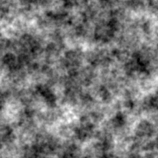
We refer the reader to Figure 2 for the simulated map of cosmic strings (no junctions) plus Gaussian inflationary perturbations. The map is for a value $G\mu=10^{-7}$.

Figure 2: Temperature map in a model with both cosmic strings ($N=10$ and $G\mu=10^{-7}$, no junctions) and Gaussian fluctuations.

Next we describe the simulations in the presence of junctions. The first difference is that not all strings have the same tension. By $\mu_{i}$ we will denote the tension of the i’th string. The vector ${\bf{\mu_{i}}}$ has magnitude $\mu_{i}$ and points in direction of the string. We will take the total number of string segments per Hubble volume to be $N=10$. We assume junctions in the shape of a “Y”, i.e. junctions with three legs each. Thus, there will be one string segment per Hubble volume which is not part of a junction.

As in the string simulation without junctions, the beginning of the first string in the junction is placed randomly within a window extending by one Hubble length in each direction around the observed window. This accounts for strings which might begin within the field of view and extend out of it and for strings which might begin outside the field of view and extend into the observed window. The first string’s starting point in this simulation will be the point where the three strings meet. The angle and sign of its velocity vector as well as the direction of the string are randomly determined. The string’s velocity angle and sign determine which of the two boxes around the string will be assigned a positive and which a negative temperature fluctuation compared to the average. The formula (3) taken from Brandenberger:2007ae to determine which side of the string has a positive temperature difference compared to the average is:

$$\frac{\delta T}{T}\,=\,8\pi G\gamma|\bm{v}\cdot(\bm{\mu_{i}}\times\bm{k})|$$ (3)

in which $\bm{v}$ is the velocity vector of the string, and $\bm{k}$ is the line of sight unit vector perpendicular to the observation window.

The first string segment of a junction has a fixed input string tension. We use $G\mu=8.7\times 10^{-8}$ because when there are three junctions per Hubble volume this gives a coefficient $a=0.976$. Recall that $a$ is the coefficient used to sum the Gaussian contribution of the map with the string map. A value of $a=0.976$ is obtained in the case of a simulation with $G\mu=1\times 10^{-7}$ for $N=10$ without junctions. We want to compare different maps with the same contribution from the Gaussian perturbations. Therefore we fix $a$ and compute the corresponding $G\mu$ for simulations with junctions and varying values of $N$. To determine the value of $G\mu$ for a simulation with junctions, we first perform a simulation with a given value $G\mu_{0}$ and compute the resulting value of $a$, denoted here by $a_{0}$. The value of $G\mu$ which yields the required value of $a$ is then given by:

$$G\mu^{2}\,=\,\left(\frac{a^{2}-1}{a_{0}^{2}-1}\right)(G\mu_{0}^{2})\,.$$ (4)

The value of $a$ for a given string tension and given value of $N$ will be higher than in our previous paper Danos:2008fq since the boxes of altered temperature per the KS effect are smaller in this simulation where the depth can be less than the string width. Hence, the strings contribute less power.

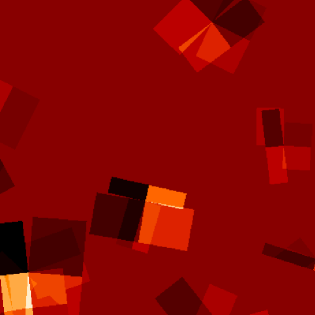
When simulating junctions, we draw the second string at the same point as the beginning of the first string with a string tension given by a random fraction of the first string’s tension. The direction of the second string is random. The third string’s direction is chosen such that the vector sum equals zero for the three vectors with magnitudes given by the string tensions and directions given by the directions of the strings. The magnitude of this third vector indicating the direction of the third string gives the string tension for the third string. Figure 3 demonstrates the temperature signature for a few strings with junctions.

Figure 3: A few cosmic strings with junctions.

As in our previous paper Danos:2008fq we lay down strings independently in each Hubble expansion time interval starting from recombination until the present time. Figure 4 shows the resulting angular power spectrum ($C_{l}$ spectrum) for a scaling solution of $N=10$, a string tension of the first string as $G\mu=8.7\times 10^{-8}$ and three junctions per Hubble volume. The value of the string tension without junctions was chosen to lie slightly below the current best upper limits; the string tension for simulations with junctions was then selected to have the same contribution of the background Gaussian perturbations.

Figure 4: The angular power spectrum of the CMB anisotropy maps for cosmic string simulations with three junctions per Hubble volume and a scaling solution with $N=10$ and $G\mu=8.7\times 10^{-8}$. The horizontal axis is $l$, the vertical axis is $l(l+1)C_{l}$.

III Canny Algorithm

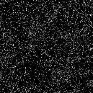
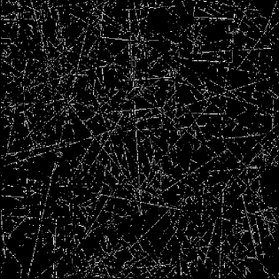
We refer the reader to Danos:2008fq for a thorough discussion of our application of the Canny algorithm. In essence, we look for edges by searching for maximal gradients larger than a threshold $t_{u}$. These local maxima are perpendicular to the direction of the edge. Gradients larger than a cutoff value, $t_{c}$, are removed as these will likely be due to the underlying Gaussian perturbations. Gradients that are between the upper threshold and a lower threshold are marked with a value of one and counted as part of an edge if they are connected to a point in a satisfactory direction (perpendicular or near perpendicular) whose gradient is a local maximum greater than or equal to the upper threshold. Our algorithm creates a map of edges, or a map of points which are marked as one connected together in edges. These can be seen for strings without junctions obeying a scaling solution of $N=10$ in Figure 5 and strings with three junctions per Hubble volume obeying a scaling solution of $N=10$ in Figure 6. Once an edge map has been created the program counts the number of continuous points that satisfy the above criteria, thus counting the number of points in the edges.

Figure 5: Pure string edge map without junctions obeying a scaling solution of N=10.

Figure 6: Cosmic string edge map with three junctions per Hubble volume obeying a scaling solution of N=10.

In our simulations, we have chosen the following values of the cutoff parameters which enter the Canny algorithm: the top cutoff is $t_{c}=3$ , the upper cutoff is $t_{u}=0.25$ and the lower cutoff is $t_{l}=0.1$. These values were chosen based on the parameter optimization performed in our previous work Danos:2008fq .

IV Density Distribution Analysis

Because strings with junctions are grouped together, we hypothesized that the distribution of edges with junctions would differ from the distribution without junctions. We divided the observation window by a grid into boxes and counted the number of edges and number of points marked as one (the number of pixels in edges) per grid box. The size of a grid box is a free parameter in our analysis. We then plotted the number of boxes versus the number of either edges or points marked as one per box. Using the number of edges or the number of points marked as one per box gives slightly different statistics.

When we count the number of edges in a given grid box, we need an algorithm to determine which box an edge falls within when edges cross boxes. We choose to assign an entire edge to the box containing a specific pixel of that edge. We could use the first pixel as the point denoting the edge, but this introduces a position bias because the algorithm counts edges starting from the bottom left of the window. However, when searching for pixels to include in an edge, the algorithm does not search in a linear fashion so the final pixel included in an edge does not have a biased position relative to the other pixels in the edge. Therefore, we assign the position of the edge to the final pixel.

We now discuss our numerical results. All of the simulations were for the same value of $a$. In all the following figures the blue (solid) curve is for $N=10$ with three junctions per Hubble volume. The other curves correspond to cosmic string simulations without junctions, the red innermost (dash dot dot) curve is for $N=1$, the yellow (dashed) one is for $N=6$, the green (dot-dashed) one is for $N=5$, and the outermost red (dotted) one is for $N=10$. All curves correspond to the average over 100 edge maps. Note that the $N=10$ curve with junctions is closest to the $N=5$ curve without junctions.

The statistic we use to determine if the curves are distinguishable is a combination of the Student t-test and the Fisher combined probability test. For each value of the x-axis (the number of points marked as one or the number of edges) we are given the mean number of boxes that contain that number of points/edges and the standard deviation. With two means and corresponding standard deviations we can apply the t-test to compute the probability $p_{l}$ that the two means originate from the same distribution. The Fisher combined probability method then computes $\chi^{2}$ as follows:

$$\chi^{2}_{2k}\,=\,-2\sum_{l=1}^{k}\ln(p_{l})$$ (5)

where $k$ is the maximal number of edges/points marked as one being which arise. We compute the probability value from the $\chi^{2}$ distribution with $2k$ values. Bins with entries or standard deviations equal to zero are obviously not included in the sum.

Figures 7-10 are pure string (no Gaussian added) histograms. We see that for the different scaling solutions the peak and the width of the curves are shifted. We also see that it is difficult to distinguish by eye between the scaling solution $N=5$ without junctions and $N=10$ with junctions, but that using the Fisher probability method these curves are clearly distinguishable.

We also see that as we change the box size (or the number of boxes in the grid) the results differ. This opens up the possibility to probe the difference between two sky maps using a set of different statistics. One statistic may be more powerful at distinguishing the map with string junctions from a map without junctions for one value of $N$, while another statistic may yield a stronger discrimination for another value of $N$.

In Figure 7 we divide the observation window into 36 by 36 size boxes and plot the number of boxes for pure string maps (without Gaussian contribution) versus the number of points marked as one in each box. Table 1 shows the corresponding probabilities for the junction maps to have come from the same distribution as the corresponding string maps without junctions for various scaling solutions. In the table, each line corresponds to a different comparison. The first column gives the parameters of the simulation with junctions (which are always taken to be the same), the second column states the parameters of the simulation without junctions which the run indicated in the first column is compared to. The third line gives the probability that the two maps come from the same distribution. A probability of zero means that the numerical result is smaller than the numerical cutoff.

Figure 8 plots the same as above except that the grid is divided into 26 by 26 boxes. Table 2 displays the results for this figure.

Figure 9 plots the histogram of the number of boxes versus the number of edges for 36 by 36 boxes in the grid. Table 3 displays the statistical results for this figure. We see that using edges instead of number of points yields an improved discriminatory power.

Figure 10 plots the histogram for the number of boxes versus the number of edges for 26 by 26 boxes in the grid with Table 4 giving the corresponding statistical results.

Figure 7: Pure string histograms for 36$\times$36 boxes. Number of boxes versus the number of points marked as one. The red innermost curve (dash dot dot) is the average over 100 edge maps for $N=1$, the blue curve (solid) is for $N=10$ with three junctions per Hubble volume, the yellow curve (dashed) is for $N=6$, the green curve (dash dot) is for $N=5$, and the outermost red curve (dotted) is for $N=10$. Only the blue curve includes the presence of junctions. See Table 1 for string tensions and $a$ coefficient.

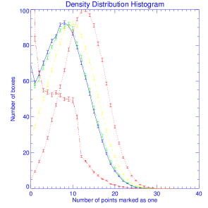
Table 1: Probabilities that Maps with Junctions come from same Distribution as Maps without Junctions for Pure Strings
Based on the distribution of points marked as 1
$a=0.976$ 36x36 Boxes Per window
$N$ $G\mu$ junctions $N$ $G\mu$ junctions probability 10 $8.7\times 10^{-8}$ yes 10 $1\times 10^{-7}$ no 0 10 $8.7\times 10^{-8}$ yes 6 $1.2\times 10^{-7}$ no 0 10 $8.7\times 10^{-8}$ yes 5 $1.37\times 10^{-7}$ no $5\times 10^{-9}$ 10 $8.7\times 10^{-8}$ yes 1 $3.12\times 10^{-7}$ no 0

Figure 8: Pure string histograms for 26$\times$26 boxes. Number of boxes versus the number of points marked as one. The red innermost curve (dash dot dot) is the average over 100 edge maps for $N=1$, the blue curve (solid) is for $N=10$ with three junctions per Hubble volume, the yellow curve (dashed) is for $N=6$, the green curve (dash dot) is for $N=5$, and the outermost red curve (dotted) is for $N=10$. Only the blue curve includes the presence of junctions.

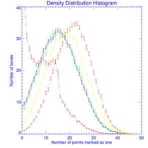
Table 2: Probabilities that Maps with Junctions come from same Distribution as Maps without Junctions for Pure Strings
(Based on the distribution of points marked as 1)
$a=0.976$ 26x26 Boxes Per window
$N$ $G\mu$ junctions $N$ $G\mu$ junctions probability 10 $8.7\times 10^{-8}$ yes 10 $1\times 10^{-7}$ no 0 10 $8.7\times 10^{-8}$ yes 6 $1.2\times 10^{-7}$ no 0 10 $8.7\times 10^{-8}$ yes 5 $1.37\times 10^{-7}$ no $3\times 10^{-6}$ 10 $8.7\times 10^{-8}$ yes 1 $3.12\times 10^{-7}$ no 0

Figure 9: Pure string histograms for 36$\times$36 boxes. Number of boxes versus the number of edges. The red innermost curve (dash dot dot) is the average over 100 edge maps for $N=1$, the blue curve (solid) is for $N=10$ with three junctions per Hubble volume, the yellow curve (dashed) is for $N=6$, the green curve (dash dot) is for $N=5$, and the outermost red curve (dotted) is for $N=10$. Only the blue curve includes the presence of junctions.

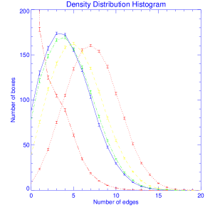
Table 3: Probabilities that Maps with Junctions come from same Distribution as Maps without Junctions for Pure Strings
(Based on the distribution of edges)
$a=0.976$ 36x36 Boxes Per window
$N$ $G\mu$ junctions $N$ $G\mu$ junctions probability 10 $8.7\times 10^{-8}$ yes 10 $1\times 10^{-7}$ no 0 10 $8.7\times 10^{-8}$ yes 6 $1.2\times 10^{-7}$ no 0 10 $8.7\times 10^{-8}$ yes 5 $1.37\times 10^{-7}$ no 0 10 $8.7\times 10^{-8}$ yes 1 $3.12\times 10^{-7}$ no 0

Figure 10: Pure string histograms for 26$\times$26 boxes. Number of boxes versus the number of edges. The red innermost curve (dash dot dot) is the average over 100 edge maps for $N=1$, the blue curve (solid) is for $N=10$ with three junctions per Hubble volume, the yellow curve (dashed) is for $N=6$, the green curve (dash dot) is for $N=5$, and the outermost red curve (dotted) is for $N=10$. Only the blue curve includes the presence of junctions.

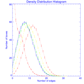
Table 4: Probabilities that Maps with Junctions come from same Distribution as Maps without Junctions for Pure Strings
(Based on the distribution of edges)
$a=0.976$ 26x26 Boxes Per window
$N$ $G\mu$ junctions $N$ $G\mu$ junctions probability 10 $8.7\times 10^{-8}$ yes 10 $1\times 10^{-7}$ no 0 10 $8.7\times 10^{-8}$ yes 6 $1.2\times 10^{-7}$ no 0 10 $8.7\times 10^{-8}$ yes 5 $1.37\times 10^{-7}$ no $8\times 10^{-16}$ 10 $8.7\times 10^{-8}$ yes 1 $3.12\times 10^{-7}$ no 0

Figures 11-14 with corresponding Tables 5-8 give the results for the string maps with Gaussian added. The string tensions are adjusted so that the $a$ coefficient remains the same for each scaling solution, hence keeping the percentage of the Gaussian contribution constant. We choose the baseline $a$ coefficient to be consistent with the string tension limits given by Pogosian, Wasserman, and Wyman (see the corresponding reference in the list limits ).

In Figure 11 the number of boxes versus number of points marked as one is plotted for 36 by 36 size boxes in a grid. We can easily distinguish between scaling solutions of $N=10$, $N=6$, and $N=1$ of maps without junctions compared to maps with three junctions per Hubble volume. With fixed 36 by 36 boxes in a 10 degree window, maps with $N=5$ are indistinguishable from maps of $N=10$ with three junctions per Hubble volume, as can be seen in Table 5.

However, here is where our power of being able to use a set of different statistics comes in handy. In Figure 12, corresponding to Table 6, we use 26 by 26 size boxes in a grid. Now, the results for $N=5$ are distinguishable from those in simulations with junctions, but the $N=10$ junction simulation results and the $N=6$ no junction scaling solution are no longer distinguishable. With the combined results for both 36 by 36 and 26 by 26 size boxes we can distinguish maps with junctions from maps without junctions for strings plus Gaussian fluctuations for all values of $N$. The explanation for our results is that the edges cluster differently on different length scales for simulations with and without junctions.

A slightly different analysis is to consider the distribution of edges versus the number of pixels in edges. With junctions we expect the edges to be longer and therefore less dense in number than the number of edges for maps without junctions. Figure 13 and its corresponding Table 7 indicate the results for number of boxes versus number of edges for 36 by 36 size boxes. From these results maps with junctions are indistinguishable from maps of a no-junction scaling solutions with $N=6$. However, Figure 14 and its corresponding Table 8 show that by plotting the number of boxes versus number of edges for 26 by 26 size boxes, maps with junctions become distinguishable from maps without junctions for all scaling solutions we considered.

Figure 11: Strings plus Gaussian histogram for 36$\times$36 boxes. Number of boxes versus the number of points marked as one. The red curve (dash dot dot) is the average over 100 edge maps for $N=1$, the blue curve (solid) is for $N=10$ with three junctions per Hubble volume, the yellow curve (dashed) is for $N=6$, the green curve (dash dot) is for $N=5$, and the outermost red curve (dotted) is for $N=10$. Only the blue curve includes the presence of junctions.

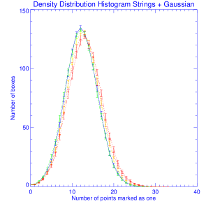
Table 5: Probabilities that Maps with Junctions come from same Distribution as Maps without Junctions for Strings with Gaussian
(Based on the distribution of points marked as 1)
$a=0.976$ 36x36 Boxes Per window
$N$ $G\mu$ junctions $N$ $G\mu$ junctions probability 10 $8.7\times 10^{-8}$ yes 10 $1\times 10^{-7}$ no $3.2\times 10^{-13}$ 10 $8.7\times 10^{-8}$ yes 6 $1.2\times 10^{-7}$ no $3.6\times 10^{-6}$ 10 $8.7\times 10^{-8}$ yes 5 $1.37\times 10^{-7}$ no $0.79$ 10 $8.7\times 10^{-8}$ yes 1 $3.12\times 10^{-7}$ no 0

Figure 12: String plus Gaussian histogram for 26$\times$26 boxes. Number of boxes versus the number of points marked as one. The red curve (dash dot dot) is the average over 100 edge maps for $N=1$, the blue curve (solid) is for $N=10$ with three junctions per Hubble volume, the yellow curve (dashed) is for $N=6$, the green curve (dash dot) is for $N=5$, and the outermost red curve (dotted) is for $N=10$. Only the blue curve includes the presence of junctions.

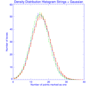
Table 6: Probabilities that Maps with Junctions come from same Distribution as Maps without Junctions for Strings with Gaussian
(Based on the distribution of points marked as 1)
$a=0.976$ 26x26 Boxes Per window
$N$ $G\mu$ junctions $N$ $G\mu$ junctions probability 10 $8.7\times 10^{-8}$ yes 10 $1\times 10^{-7}$ no 0.069915751 10 $8.7\times 10^{-8}$ yes 6 $1.2\times 10^{-7}$ no 0.70260790 10 $8.7\times 10^{-8}$ yes 5 $1.37\times 10^{-7}$ no $7.7\times 10^{-7}$ 10 $8.7\times 10^{-8}$ yes 1 $3.12\times 10^{-7}$ no 0.00011939824

Figure 13: String plus Gaussian histogram for 36$\times$36 boxes. Number of boxes versus the number of edges. The red curve (dash dot dot) is the average over 100 edge maps for $N=1$, the blue curve (solid) is for $N=10$ with three junctions per Hubble volume, the yellow curve (dashed) is for $N=6$, the green curve (dash dot) is for $N=5$, and the outermost red curve (dotted) is for $N=10$. Only the blue curve includes the presence of junctions.

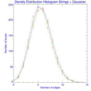
Table 7: Probabilities that Maps with Junctions come from same Distribution as Maps without Junctions Strings with Gaussians
(Based on the distribution of edges)
$a=0.976$ 36x36 Boxes Per window
$N$ $G\mu$ junctions $N$ $G\mu$ junctions probability 10 $8.7\times 10^{-8}$ yes 10 $1\times 10^{-7}$ no $7.46\times 10^{-11}$ 10 $8.7\times 10^{-8}$ yes 6 $1.2\times 10^{-7}$ no 0.76527496 10 $8.7\times 10^{-8}$ yes 5 $1.37\times 10^{-7}$ no 0.00028340182 10 $8.7\times 10^{-8}$ yes 1 $3.12\times 10^{-7}$ no $4.2\times 10^{-10}$

Figure 14: String plus Gaussian histogram for 26$\times$26 boxes. Number of boxes versus the number of edges. The red curve (dash dot dot) is the average over 100 edge maps for $N=1$, the blue curve (solid) is for $N=10$ with three junctions per Hubble volume, the yellow curve (dashed) is for $N=6$, the green curve (dash dot) is for $N=5$, and the outermost red curve (dotted) is for $N=10$. Only the blue curve includes the presence of junctions.

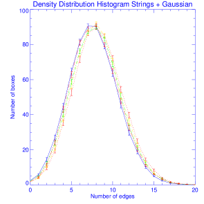
Table 8: Probabilities that Maps with Junctions come from same Distribution as Maps without Junctions for Strings with Gaussian
(Based on the distribution of edges)
$a=0.976$ 26x26 Boxes Per window
$N$ $G\mu$ junctions $N$ $G\mu$ junctions probability 10 $8.7\times 10^{-8}$ yes 10 $1\times 10^{-7}$ no 0 10 $8.7\times 10^{-8}$ yes 6 $1.2\times 10^{-7}$ no 0 10 $8.7\times 10^{-8}$ yes 5 $1.37\times 10^{-7}$ no $4.1\times 10^{-8}$ 10 $8.7\times 10^{-8}$ yes 1 $3.12\times 10^{-7}$ no 0.00076553716

V Conclusions

We have applied the Canny algorithm to simulated maps of CMB anisotropies induced by models with cosmic stings either containing or not containing string junctions. We proposed a statistic with which it should be possible to distinguish between the maps with and without junctions. This provides a method with which one can distinguish between the predictions of simple gauge field theory models with cosmic strings (which typically do not admit string junctions), and models such as those giving rise to cosmic superstrings, which are characterized by the presence of junctions.

We first showed that our statistic is able to clearly differentiate between string maps with and without junctions in the absence of Gaussian noise. However, since we know that a cosmic string model without a dominant Gaussian contribution to the spectrum of fluctuations is not consistent with the latest data on the angular power spectrum of CMB anisotropies, we need to consider correctly normalized sky maps which contain strings with a tension sufficiently low such that its contribution to the power spectrum does not exceed the current limits limits , with the bulk of the power coming from Gaussian noise. In this case it is more difficult to differentiate between maps where the strings have junction and where they do not.

Nevertheless, making use of our detailed statistics, we found a clear distinction in the shape (peak and width) of the density distribution (number of boxes sampled with varying numbers of edges or pixels in the edges) for the different scaling solutions. For example, $N=1$ strings per Hubble volume had a large number of boxes with just a few edges, as would be expected, whereas $N=10$ strings per Hubble volume looked more Gaussian, as expected. We found a statistical difference between the curves for junctions and the curves of different scaling solutions without junctions.

Future work includes optimizing the Canny algorithm, and searching for the lowest value of the string tension for which maps with and without string junctions can be differentiated. It would also be very interesting to algorithms to “real” string simulations (those obtained via a numerical evolution of the Nambu-Goto equations) rather than just relying on the simple toy models for the distribution of strings which we have used. Maps of CMB anisotropies produced by strings without junctions coming from “real” simulations are available Fraisse . However, to our knowledge there are no corresponding results for networks with string junctions.