Discontinuous nonequilibrium phase transitions in a nonlinearly pulse-coupled excitable lattice model

Abstract

We study a modified version of the stochastic susceptible-infected-refractory-susceptible (SIRS) model by employing a nonlinear (exponential) reinforcement in the contagion rate and no diffusion. We run simulations for complete and random graphs as well as $d$-dimensional hypercubic lattices (for $d=3,2,1$). For weak nonlinearity, a continuous nonequilibrium phase transition between an absorbing and an active phase is obtained, such as in the usual stochastic SIRS model [Joo and Lebowitz, Phys. Rev. E 70, 036114 (2004)]. However, for strong nonlinearity, the nonequilibrium transition between the two phases can be discontinuous for $d\geq 2$, which is confirmed by well-characterized hysteresis cycles and bistability. Analytical mean-field results correctly predict the overall structure of the phase diagram. Furthermore, contrary to what was observed in a model of phase-coupled stochastic oscillators with a similar nonlinearity in the coupling [Wood et al., Phys. Rev. Lett. 96, 145701 (2006)], we did not find a transition to a stable (partially) synchronized state in our nonlinearly pulse-coupled excitable elements. For long enough refractory times and high enough nonlinearity, however, the system can exhibit collective excitability and unstable stochastic oscillations.

I Introduction

Understanding collective effects of noisy excitable elements is essential for several disciplines, such as neuroscience, epidemiology, and chemistry, among others. An isolated excitable element is a dynamical system which stays in a quiescent state until it suffers a sufficiently strong perturbation. In that case its trajectory in phase space can be characterized by an excited state, which is then followed by a refractoriness to further perturbations before returning to rest. A minimal (discrete) model of an excitable element therefore consists of a three-state system Lindner et al. (2004). In the parlance of neuroscience (epidemics), each element could represent a neuron or patch of active membrane (individual) which sequentially becomes polarized (susceptible), spiking or depolarized (infected), and then refractory (recovered). Collective dynamics emerge because quiescent elements are typically perturbed by excited elements.

A simple system which incorporates these ingredients in a scenario with noise is the stochastic susceptible-infected-recovered-susceptible (SIRS) epidemic lattice model Joo and Lebowitz (2004). It is a continuous-time model in which a site goes from susceptible to infected at a rate which depends on the density of its infected neighbors. In epidemiology, the model (or variants thereof) can be employed to investigate, e.g., whether an initial density of infected sites (which is usually chosen as the order parameter) will reach a nonzero stationary value or decrease to zero. If all sites become quiescent, the dynamic halts and the system is said to be in a absorbing state Marro and Dickman (1999).

Increasing the coupling between infected and susceptible sites, the SIRS model undergoes a continuous nonequilibrium phase transition from an absorbing to an active phase characterized by a stationary nonzero density of infected sites. However, experimental data (from neuroscience, epidemiology, and chemistry, among others) can exhibit also global oscillations. This additional transition has been observed mostly in cellular automata, where the sites are synchronously updated Lewis and Rinzel (2000); Kuperman and Abramson (2001); Lindner et al. (2004); Kinouchi and Copelli (2006). This technical detail is apparently relevant since global oscillations in stochastic continuous-time models are less common. As discussed by Risau-Gusman and Abramson, they sometimes appear as stochastic oscillations in single runs of the model but disappear in trajectories of the averaged lattice activity and analytical descriptions (usually mean-field) thereof Risau-Gusman and Abramson (2007). Global oscillations predicted by mean-field (MF) approximations were observed in both non-Markovian Prager et al. (2003) and Markovian Wood et al. (2006) models of three-state continuous-time stochastic oscillators. These models, however, do not have an absorbing state.

Figure 1: (Color online) Phase space $[P(S),P(I)]$ showing the nullclines $\dot{P}(I)=0$ (dashed lines) and $\dot{P}(S)=0$ (dot-dashed lines). Grey triangles corresponds to the physically acceptable region $0\leq P(I)\leq 1-P(S)$. In each row, $a$ is kept constant and $b$ increases from left to right. In the lower panel (b) ($a=0.5$), the absorbing state at $P(S)=1$ loses stability in a transcritical bifurcation as $b$ increases. In the upper panel (a) ($a=2.25$), the $\dot{P}(I)=0$ nullcline is bent by the exponential nonlinearity [see eq. 4], creating an active state with finite $P(I)$ in a saddle-node bifurcation. Closed (open) symbols denote stable (unstable) fixed points. Note that the nullcline $\dot{P}(I)=0$ always comprises the line $P(I)=0$. When the absorbing state is unstable (a saddle), $P(I)=0$ corresponds to its stable manifold (rightmost column). Except for this case, the trajectories (solid lines) represent the stable and unstable manifolds of the saddles.

Here we investigate a modified version of the SIRS model with a nonlinear rate which can be considered a pulse-coupled excitable version of the original phase-coupled oscillator model of Wood et al. Wood et al. (2006). We will show, on the one hand, that this nonlinear (but Markovian) extension of the SIRS model is apparently insufficient for the generation of sustained collective oscillations. On the other hand, the model presents phase transitions into an absorbing state which can be continuous (if weakly nonlinear) or discontinuous (if nonlinear enough and for $d\geq 2$). We therefore provide a three-state continuous-time model which can undergo discontinuous phase transitions like those of Bidaux et al. for a two-state cellular automaton Bidaux et al. (1989) except that the nature of the transition here can be controlled by a free parameter (not only the spatial dimension Bidaux et al. (1989)). Moreover, differently from most models presenting nonequilibrium discontinuous phase transitions Dickman and Tomé (1991); Ódor et al. (1993); Marro and Dickman (1999), the parameter which controls the nature of the transition is not diffusion (which is absent from our model). The model can also exhibit a different bifurcation scenario from what is usually observed in nonequilibrium lattice models, showing collective excitability and unstable global oscillations.

The paper is organized as follows. In Sec. II we introduce the model, analyze its mean-field solution, and compare it to simulations of random and complete graphs. Simulation results for $d$-dimensional hypercubic lattices are shown in Sec. III, while our concluding remarks are discussed in Sec. IV.

II Model

In the conventional stochastic version of the SIRS epidemic model, a susceptible ($S$) site at position $x$ ($x=1,\ldots,N$) becomes infected ($I$) at a rate $\lambda n_{I}(x)/k(x)$, where $k(x)$ is the number of neighbors of $x$, out of which $n_{I}(x)$ are infected, and $\lambda$ is the so-called infection rate (the coupling parameter). After that, the site becomes temporarily insensitive to its surroundings (hence the term pulse coupling), jumping from infected to recovered ($R$) at a constant rate $\delta$, and from recovered back to susceptible at a rate $\gamma$. This is summarized as follows:

$$S\longrightarrow I \mbox{at rate }\lambda n_{I}/k,$$ (1)

$$I\longrightarrow R \mbox{at rate }\delta,$$ (2)

$$R\longrightarrow S \mbox{at rate }\gamma.$$ (3)

Since all rates could in principle be normalized by $\delta$, in the following we set $\delta=1$ without loss of generality.

For low values of $\lambda$, an initial density of infected sites eventually dies out and the system reaches its unique absorbing state (all sites susceptible). For $\lambda$ larger than a critical value $\lambda_{c}$, on the other hand, a phase with nonzero density of infected sites becomes stable in the thermodynamic limit $N\to\infty$ (though the absorbing state is obviously always a solution). The transition at $\lambda_{c}$ (studied in detail by Joo and Lebowitz Joo and Lebowitz (2004)) is widely believed to be continuous and belonging to the directed percolation (DP) universality class Assis and Copelli (2008); de Souza and Tomé .

Adapting the nonlinear coupling employed by Wood et al. Wood et al. (2006) to pulse-coupled excitable elements, one obtains a generalization of the SIRS model. Instead of Eq. 1, we propose

$$S\longrightarrow I\mbox{ at rate}$$

$$g\left(n_{I}/k,n_{S}/k\right)\equiv b\left[e^{a(n_{I}-n_{S})/k}-e^{-an_{S}/k}\right],$$ (4)

where $a$ and $b$ are coupling parameters, $n_{S}$ is the number of susceptible neighbors, and Eqs. 2 and 3 remain unaltered. Note that the interaction occurs only among first neighbors. The second term in rate 4 guarantees the existence of an absorbing state: if all sites are susceptible (thus $n_{I}=0$ for all sites), they will remain susceptible forever. For small values of $a$ ($a\ll 1$), one recovers the linear behavior of the original SIRS model, with $\lambda\simeq ab$, to first order. So for small $a$, increasing $b$ leads to a continuous phase transition just like in the SIRS model Joo and Lebowitz (2004). For large enough $a$, however, we will show that increasing $b$ leads to a discontinuous phase transition.

As a motivation to rate 4, let us note that the dynamics underlying neuronal firing is highly nonlinear in several of its aspects: membrane depolarizes when (typically Na⁺) channels open very quickly, in a thresholdlike behavior. This process, on its turn, is triggered by a (nonlinear) sum of smaller depolarizations induced at synapses by presynaptic neurons. Synaptic dynamics (including neurotransmitter binding, in the simplest case) is itself nonlinear. It is therefore not unusual that reduced models of collective neuronal phenomena allow for nonlinear terms Gerstner and Kistler (2002). In our case, the nonlinearity is controlled by parameter $a$.

II.1 Mean-field analysis

The structure of the phase diagram in the $(a,b)$ plane can be captured most easily by analyzing the mean-field version of the model. Letting $P(\alpha)$ be the probability that a site is in state $\alpha$ ($\alpha\in\{S,I,R\}$), one obtains

$$\dot{P}(S) = -g[P(I),P(S)]P(S)+\gamma P(R),$$ (5)

$$\dot{P}(I) = g[P(I),P(S)]P(S)-\delta P(I),$$ (6)

$$\dot{P}(R) = \delta P(I)-\gamma P(R).$$ (7)

These equations are exact for a complete graph when $k=N\to\infty$ and $n_{\alpha}\to\infty$ with $n_{\alpha}/k=P(\alpha)$. In what follows, we will employ the stationary value of the density of infected sites $P(I)^{*}$ as the order parameter.

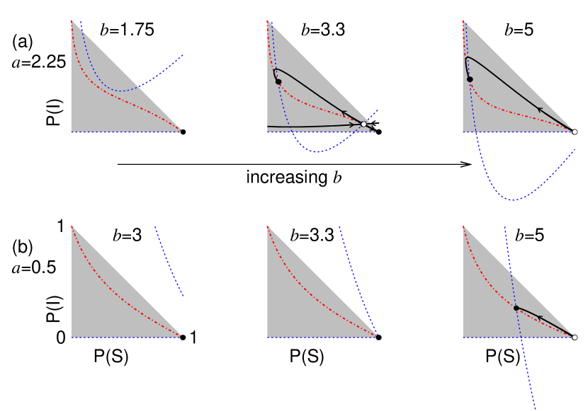
By employing the normalization condition $P(S)+P(I)+P(R)=1$, one can eliminate $P(R)$ and study the resulting two-dimensional flow of the mean-field dynamics in the $[P(S),P(I)]$ plane, as shown in Fig. 1. For low values of $a$ (lower panel of Fig. 1), the absorbing state $P(S)=1$ loses stability in a transcritical bifurcation, giving rise to a stable active state with a density of infected sites which increases continuously from $P(I)=0$. For large enough $a$, the discontinuous character of the phase transition reveals itself in the mean-field equations through a saddle-node bifurcation (upper panel of Fig. 1): an active state appears with nonzero $P(I)$, while the absorbing state remains stable. As usual, this bistability is regulated by the stable manifold of the saddle, which separates the basins of attraction of the two stable fixed points. Increasing $b$ further, another transcritical bifurcation occurs: the absorbing state loses stability and the active state becomes the only attractor of the system.

Figure 2: (Color online) Phase diagram of the (mean-field version of the) model. The dashed line marks the onset of phase bistability, with the sudden appearance of a stable active phase with finite order parameter [saddle-node bifurcation in Eqs. 5-7]. Solid lines denote a transition in which the absorbing state loses stability [transcritical bifurcation in Eqs. 5-7]. Symbols correspond to simulations in a random graph with $\gamma=1$, $K=10$, $N=10^{4}$, $t_{max}=5\times 10^{3}$, and $h=10^{-5}$ averaged over five runs. The lower (upper) inset shows the order parameter $P(I)^{*}$ for a cyclic change in the coupling parameter $b$, showing a continuous (discontinuous) transition for a small (large) value of $a$. Upward (downward) triangles: increasing (decreasing) $b$.

II.2 Random graph simulations

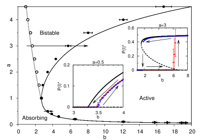
Hysteresis is one of the simplest fingerprints of multistability, and in this system it can be clearly detected in simulations of Erdős-Rényi random graphs Albert and Barabási (2002) with finite average connectivity $K$, with which the mean-field equations show a good agreement. Simulations were performed for a fixed value of $a$. For each value of $b$, we allowed the system to evolve during $t_{max}$ time steps. Each time step $\Delta t$ (corresponding to $N$ random updates Marro and Dickman (1999)) was chosen to be $(\delta+\gamma+be^{a})^{-1}$ to make sure probabilities are less than one. Parameter $b$ was increased or decreased in constant intervals $\delta b$, and the initial condition of the network for each value corresponded to the final condition of the preceding case. We applied a small rate $h$ ($h<1/N$) to spontaneously excite quiescent sites, thus preventing the system from getting trapped in the absorbing state by finite-size fluctuations Bidaux et al. (1989); Takeuchi (2008).

The insets of Fig. 2 show that a loop in $b$ leads to a hysteresis cycle [as observed for the density of active sites $P(I)$] for high enough values of $a$ ($a>a_{c}$). For low values of $a$, the phase transition is continuous. The boundaries between the phases in the $(a,b)$ plane (main plot of Fig. 2) can be numerically obtained from the mean-field equations and easily estimated from the random graph simulations (hysteresis cycles did not change significantly when $t_{max}$ was doubled; see also Sec. III).

To obtain the phase diagram shown in Fig. 2, we employed a mean refractory time comparable to the excitation time, $\gamma=1$. However, we did not find qualitative differences in the mean-field phase diagram in the limiting case $\gamma\to\infty$, which suggests that the simulation results we present here will also be valid for a two-state system.

II.3 Absence of sustained global oscillations

Figure 3: (Color online) (a) Phase diagram of the (mean-field version of the) model for $\gamma=0.01$ (panels b–g also show single-run simulations of a complete graph with $N=10^{6}$). Bifurcations are as in Fig. 2, except for those additionally occurring within the marked rectangle (inset): for increasing $b$, a saddle-node bifurcation (dashed line) is followed by a Hopf (H) bifurcation (dotted line), after which a homoclinic (HC) bifurcation occurs (see text). The absorbing phase corresponds to the grey region. The labels (b)–(d) in the inset show the points in parameter space which correspond to the phase portraits below. (b) A saddle and an unstable fixed point are born in a saddle-node bifurcation. (c) The fixed point becomes stable via a Hopf bifurcation and is surrounded by an unstable limit cycle. (d) After a homoclinic bifurcation, the limit cycle disappears. UUM = upper unstable manifold of the saddle; USM = upper stable manifold of the saddle; ULC = unstable limit cycle; LSM = lower stable manifold. The scale in (b) also applies (apart from a translation) to (c) and (d). The lower unstable manifold of the saddle always goes to the absorbing fixed point. Panels e, f, and g show time series for simulated trajectories, respectively, shown in panels b, c, and d, with examples of collective excitability and stochastic oscillations (see text for details).

In the process of scanning parameter space in search of collective oscillations, we have found small regions in which a Hopf bifurcation involving the active state can indeed occur. As we shall see, however, this does not necessarily imply the existence of sustained collective oscillations, which we have not found in this model.

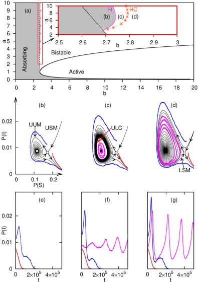
We exemplify with results for $\gamma=0.01$, whose phase diagram is shown in Fig. 3a. Though qualitatively similar to Fig. 2, there is now a narrow interval of $b$ values (for high values of $a$) in which the route to bistability, instead of the simple saddle-node scenario described in Fig. 1(a), requires additional intermediate bifurcations  [inset of Fig. 3(a)]. These occur while the absorbing fixed point remain stable.

Starting from the absorbing phase and increasing $b$, first a saddle-node bifurcation occurs in which the node is unstable [and quickly becomes a spiral, Fig. 3(b)]. At this stage, the system still has only a single stable fixed point, but the structure of phase space is such that the system has become collectively excitable: if the system is below the upper stable manifold (USM) of the saddle [Fig. 3(b)], it will monotonously return to the absorbing state, whereas a point above the USM will go through a long excursion around the upper unstable manifold (UUM) before coming to rest [Fig. 3(b)], displaying a spike-like time series [Fig. 3(e)].

Increasing $b$ further, the spiral becomes stable in a Hopf bifurcation and is now surrounded by an unstable limit cycle (ULC) [Fig. 3(c)]. Formally, in this parameter region the system is collectively bistable, but note that the active phase will only be reached from initial conditions within the ULC [which, owing to the small value of $\gamma$, is also very small — see scale in Fig. 3(b)]. Note also that the overcrowding of lines outside the ULC signals that it is weakly repulsive. The inner stable fixed point (the active phase) is correspondingly weakly attractive (which is the reason why the flux inside the ULC is not shown). This means that a collective oscillation solution exists (the ULC) but is so weakly unstable that it might get confounded with sustained oscillations [even in the numerical integration of eqs. 5-7]. From single-run simulations of a complete graph with $N=10^{6}$, we have obtained a time series with oscillations [Fig. 3(f)] which only disappear when, owing to finite-size fluctuations, the system reaches the absorbing state Marro and Dickman (1999). We therefore confirm the scenario predicted by Risau-Gusman and Abramson: since the eigenvalues of the stable fixed point have a nonzero imaginary component, inevitable fluctuations will generate stochastic oscillations Risau-Gusman and Abramson (2007).

Finally, the ULC disappears in a homoclinic (HC) bifurcation, after which the active fixed point is separated from the absorbing fixed point only by the stable manifolds of the saddle. Note that the lower stable manifold [LSM, see Fig. 3(d)] no longer comes from the unstable fixed point nor from the ULC but rather joins the USM as $t\to-\infty$. The LSM will gradually unfold as $b$ increases until a phase portrait similar to that of the central plot of Fig. 1a is reached (before the saddle collides – for yet larger values of $b$ – with the absorbing fixed point in a transcritical bifurcation). Collective excitability and stochastic oscillations remain present in this regime [Figs. 3(d) and 3(g)].

Our phase diagram emerged essentially from local stability analysis, so in principle it does not exclude a saddle-node bifurcation of cycles from occurring within the active or bistable regions. However, numerical integration of Eqs. 5-7 for a variety of initial conditions and combination of parameters did not show any signs of it.

Although the above analysis is based on the mean-field approximation, it is worth mentioning that improvements on the mean-field approximation do not necessarily help the prediction of collective oscillations. Rozhnova and Nunes Rozhnova and Nunes (2009a) recently observed that the equations obtained by Joo and Lebowitz Joo and Lebowitz (2004) for the two-site approximation lead to sustained oscillations in a small region for $\gamma\ll 1$. However, when simulating random graphs in the same parameter region, these oscillations get damped Rozhnova and Nunes (2009b).

III Simulations in hypercubic lattices

Figure 4: (Color online) Simulations for $d=3$ with $N=25^{3}$ and $h=2.5\times 10^{-5}$. (a) ($a=4.5$, averaged over 20 runs) The length of the hysteresis cycle $\Delta b$ decreases for increasing $t_{max}$ ($\Delta b$ denoted by the horizontal arrow for $t_{max}=10^{5}$). Upward (downward) triangles denote increasing (decreasing) $b$. Vertical lines show values of $b$ employed in panels (c) and (d). (b) Dependence of $\Delta b$ on $t_{max}$ is qualitatively different for $a$ above (filled circles) and below (open circles) $a_{c}$, respectively, showing a nonzero or zero asymptotic value in the limit $t_{max}\to\infty$. The lower plot is well fitted by a power law with exponent 0.55. Note that the precision in $\Delta b$ is limited by the increment in $b$ employed in the hysteresis cycle ($\delta b=1.8\times 10^{-3}$ in the case $a=1.875$). Panels (c) and (d) show the time evolution of $P(I)$ (averaged over 20 runs) for $a=4.5$ and different initial conditions [with $NP(I)$ sites in state $I$ at $t=0$ and the remaining in state $S$], showing phase bistability for $b=3.25$ but not for $b=7$.

Figure 5: (Color online) Simulations for $d=2$ with $N=150^{2}$ and $h=2.5\times 10^{-5}$. (a) ($a=7$, averaged over 10 runs) The length of the hysteresis cycle $\Delta b$ decreases for increasing $t_{max}$ ($\Delta b$ denoted by the horizontal arrow for $t_{max}=2\times 10^{5}$). Upward (downward) triangles denote increasing (decreasing) $b$. Vertical lines show values of $b$ employed in panels (c) and (d). (b) Dependence of $\Delta b$ on $t_{max}$ is qualitatively different for $a$ above (filled circles) and below (open circles) $a_{c}$, respectively, showing a nonzero or zero asymptotic value in the limit $t_{max}\to\infty$. The lower plot is well fitted by a power law with exponent 0.63. Note that the precision in $\Delta b$ is limited by the increment in $b$ employed in the hysteresis cycle ($\delta b=10^{-2}$ in the case $a=4.5$). Panels (c) and (d) show the time evolution of $P(I)$ (averaged over 20 runs) for $a=7$ and different initial conditions [with $NP(I)$ sites in state $I$ at $t=0$ and the remaining in state $S$], showing phase bistability for $b=4.4$ but not for $b=21.5$.

Figure 6: (Color online) Phase diagram of the model in one-, two- and three-dimensional hypercubic lattices (squares, circles and triangles, respectively). Open symbols (with dashed lines to guide the eye) mark the onset of phase bistability, with the sudden appearance of a stable active phase with finite order parameter. Filled symbols (with solid lines to guide the eye) denote a transition in which the absorbing state loses stability. The region in between dashed and solid lines correspond to the bistable regime. Lines without symbols show MF results for comparison. Results correspond to simulations with $\gamma=1$ and $h=2.5\times 10^{-5}$. For $d=1$, 2, and 3, linear system sizes were $L=32400$, $L=150$, and $L=25$ (where $N=L^{d}$), the maximum values of $t_{max}$ were $5\times 10^{5}$, $2\times 10^{5}$, and $10^{5}$, with results averaged over 10, 10, and 20 runs, respectively.

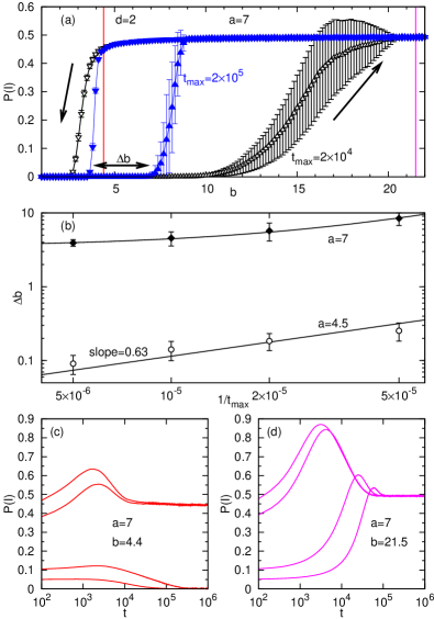
Since simulations with small values of $\gamma$ are very difficult to perform Joo and Lebowitz (2004), we now focus on the simpler bifurcation scenario of Fig. 2 and discuss the results of simulations for $\gamma=1$. Identifying the nature of the transition in hypercubic lattices is not so simple as for random and complete graphs. As has been recently discussed in detail by Takeuchi Takeuchi (2008), even a system which undergoes a continuous phase transition into an absorbing state (such as those belonging to the directed percolation universality class) may show a hysteresis cycle when the coupling parameter loops around its critical value. This is due to the divergence of the transient times at criticality in the thermodynamic limit. In simulations, this gets reflected in the width of the hysteresis cycle scaling with the ramp rate (defined as the increment in $b$ per unit time) as $(1/t_{max})^{1/(\beta+1)}$, where $\beta$ is the critical exponent governing the order parameter Takeuchi (2008); Marro and Dickman (1999).

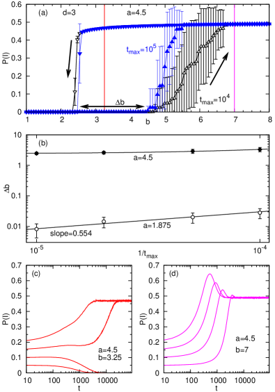
Consider, for instance, the hysteresis cycles shown in Fig. 4(a) for $d=3$ and two values of $t_{max}$ differing by an order of magnitude (while the increments in the values of $b$ have been kept the same Takeuchi (2008)). Whether or not the transition is continuous will depend on whether the width $\Delta b$ of the hysteresis cycle shrinks to zero in the limit $t_{max}\to\infty$. We have operationally defined $\Delta b$ as follows: for each run, we attribute the upper end of the hysteresis cycle to the $b$ value at which the density of active sites (averaged over $t_{max}$ time steps) $P(I)$ is first above $1/\sqrt{N}$. Similarly, the lower end of the hysteresis cycle is defined as the point where $P(I)$ falls below $1/\sqrt{N}$. The width of the hysteresis cycle $\Delta b$ is then obtained by averaging the difference over the runs. We plotted $\Delta b$ versus $1/t_{max}$ in Fig. 4(b) for two values of $a$. For $a=4.5$ [which corresponds to the hysteresis cycles shown in Fig. 4(a)], a linear extrapolation leads to a nonzero value of $\Delta b$ as $t_{max}\to\infty$, which is consistent with a discontinuous phase transition. For $d=3$ and $a=1.875$, on the other hand $\Delta b$ decreases to zero as a power law $(1/t_{max})^{0.55}$, which is consistent with Takeuchi’s prediction Takeuchi (2008) for the DP universality class [$\beta\simeq 0.805(10)$ Jensen (1992)].

One could in principle feel uncomfortable with the above described criterion for deciding on the discontinuity of the transition because in practice the linear extrapolation may not coincide with $\lim_{t_{max}\to\infty}\Delta b$ if transient times are too long (and we expect them to be long near a continuous transition!). This problem becomes more salient as we decrease the spatial dimension, as depicted for $d=2$ and $a=7$ in Fig. 5. Note the smoothness of the largest hysteresis cycle in Fig. 5(a), which is very similar to the ones observed by Takeuchi Takeuchi (2008) near a continuous transition. According to the extrapolated value of $\Delta b$ for $t_{max}\to\infty$, however, this transition would be considered discontinuous [see upper plot in Fig. 5(b)], whereas for weaker nonlinearity [$a=4.5$, lower plot of Fig. 5(b)] we obtain again a power law $(1/t_{max})^{0.63}$ Takeuchi (2008) compatible with DP in $d=2$ [$\beta\simeq 0.583(4)$ Jensen (1992)].

To be sure of the discontinuity of the transition, it is simpler (and computationally less expensive) to investigate directly the alleged bistability: we fix $a$ and $b$ and check the dependence of the stationary state on the initial condition Dickman and Maia (2008); Ódor and Dickman (2009). This test is shown in Figs. 4(c), 4(d), 5(c), and 5(d) for $d=3$ and $d=2$, respectively. Figures 4(c) and 5(c) confirm bistability since for lower (higher) initial values of $P(I)$ the system converges to the absorbing (active) state. Figures 4(d) and 5(d) serve as a negative control, confirming (in a region where only the active state is stable) that the convergence to the absorbing state in the previous cases are not due to finite-size fluctuations. We note that all samples converged to the same attractor (either absorbing or active) as their average.

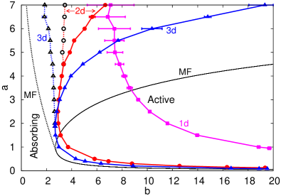
The extrapolation $\lim_{t_{max}\to\infty}\Delta b$ was employed to draw the phase diagram of the model for two- and three-dimensional lattices. As shown in Fig. 6, the qualitative structure of the phase diagram is well reproduced by the mean-field predictions, though quantitative agreement worsens as dimensionality decreases as expected. Note that the bistable phase for $d=2$ is much smaller than for $d=3$. For $d=1$, the large error bars in Fig. 6 for large $a$ emerge due to extremely large transients. We have not observed clearly discontinuous transitions for $d=1$ up to $a=7$. This is in agreement with the results of Bidaux et al. Bidaux et al. (1989); Jensen (1991), as well as with Hinrichsen’s conjecture that discontinuous transitions in $d=1$ should only occur in the presence of diffusion Hinrichsen .

IV Conclusions and perspectives

In summary, we have proposed a Markovian continuous-time lattice model of nonlinearly pulse-coupled excitable elements. Coupling depends linearly on rate $b$ and nonlinearly on the dimensionless parameter $a$. We have shown that increasing the nonlinearity of the coupling leads to a change in the nature of the phase transition into an active state. In the regime of linear coupling ($a\ll 1$), where the model approaches the stochastic SIRS model, an active phase with $P(I)>0$ appears through a continuous transition as $b$ increases. In a sufficiently nonlinear regime (large enough $a$), increasing $b$ leads to a discontinuous phase transition. The nature of the transition can therefore be controlled by a single parameter, which is not diffusion. These results can be predicted by mean-field analysis and are qualitatively confirmed in simulations of random graphs and hypercubic lattices for $d\geq 2$. The fact that a discontinuous transition was not found for $d=1$ is consistent with previous results for two-state systems with little or no diffusion Bidaux et al. (1989); Jensen (1991); Dickman and Tomé (1991); Ódor et al. (1993); Hinrichsen .

We have characterized discontinuous transitions by two complementary criteria: first, hysteresis cycles were obtained and their width estimated by extrapolation for an infinite number of Monte Carlo time steps; then, bistability was explicitly confirmed by checking that the system trajectory exhibits dependence on the initial conditions. In the case of continuous transitions, the width of the hysteresis cycles scaled with the ramp rate according to recent predictions by Takeuchi Takeuchi (2008).

Finally, we recall that the exponential coupling in Eq. 4 was inspired in the model of Wood et al. Wood et al. (2006). While their nonlinear phase-coupled stochastic oscillators do undergo a phase transition into a synchronized state, we did not find sustained collective oscillations with a similar nonlinearity among pulse-coupled excitable elements. However, we did find (albeit in a small parameter region) unstable global oscillations and collective excitability in the mean-field equations. Simulations of the complete graph revealed stochastic oscillations in single runs whenever the active phase corresponded to a stable spiral in the mean-field equations. It remains to be investigated whether collective excitability and stochastic oscillations remain in regular lattices or appear in the transition to a small-world regime.