Neutral modes edge state dynamics through quantum point contacts

Abstract

Dynamics of neutral modes for fractional quantum Hall states is investigated for a quantum point contact geometry in the weak- backscattering regime. The effective field theory introduced by Fradkin-Lopez for edge states in the Jain sequence is generalized to the case of propagating neutral modes. The dominant tunnelling processes are identified also in the presence of non-universal phenomena induced by interactions. The crossover regime in the backscattering current between tunnelling of single-quasiparticles and of agglomerates of $p$-quasiparticles is analysed. We demonstrate that higher order cumulants of the backscattering current fluctuations are a unique resource to study quantitatively the competition between different carrier charges. We find that propagating neutral modes are a necessary ingredient in order to explain this crossover phenomena.

1 Introduction

The Fractional Quantum Hall Effect (FQHE) represents one of the most important examples of strongly correlated electron systems [1, 2, 3]. Due to the purely two-dimensional electron motion a wider class of symmetries, for the exchange of identical particles, are admissible in comparison with the three-dimensional case [4]. This implies the existence of quantum fluids with unique properties, such as fractional charges and fractional statistics, and eventually different internal topological orders [5] at a given filling factor [6]. In order to discriminate among these different theories it is useful to investigate and characterize the edge state dynamics [7]. Indeed, one may achieve unique information about the bulk properties via the holographic principle [8], by studying the low energy gapless excitations at the boundaries of the Hall bar [9, 10].

Edge states are described in terms of bosonic modes of a Chiral Luttinger Liquids ($\chi$LL) [11]. For the description of the Laughlin sequence [1] with filling factor $\nu=1/(2m+1)$ ($m\in{\bf{N}}$), only a single charged mode is necessary. Here, theoretical predictions of transport properties, as current and noise, through a Quantum Point Contact (QPC) were proposed [12, 13] and confirmed by experimental measurements [14, 15]. It was demonstrated that, in the weak-backscattering regime, the tunnelling carriers have a fractional charge $e^{*}=\nu e$ ($e$ electron charge), giving the first confirmation of charge fractionalization [1]. Further experiments [16] attempted to demonstrate also the anyonic nature of these excitations [17].

For the Jain’s sequence [18] with $\nu=p/(2mp+1)$ and $p\in{\bf{N}}$ one needs additional bosonic neutral modes in order to fulfil the hierarchical structure [19]. As suggested by Wen and Zee [20], one can introduce $p-1$ neutral modes in addition to the charge one. The model predicts the expected value $e^{*}=\nu e/p$ for the charge of the fundamental quasi-particle (qp) excitation, however, due to the increasing number of fields, for increasing hierarchy $p$, the conserved currents grows indefinitely [21, 22], creating some problem of consistency  [23]. Some predictions of this theory have been experimentally verified by investigating the transport properties in cleaved-edge overgrown devices but, at the same time, experiments shed light on the limits of the model [24, 25]. In particular the behaviour of the tunnelling current suggests that the dynamics of neutral modes is less relevant with respect to the prediction [12, 26]. These problems triggered additional theoretical investigations devoted to clarify the reasons of the discrepancies  [27]. Among them, it is important to mention the model proposed by Fradkin-Lopez (FL model) [23], which introduces only two neutral topological modes (one for infinite edge length [28]), instead of the above dynamical $p-1$ modes. These modes have zero velocity, then they do not contribute to the dynamical response, having only a role in enforcing the appropriate statistical properties. This model predicts also the correct value of the single-qp charge in agreement with the first experimental observations on tunnelling through a QPC [29]. However, successive experiments [30, 31] have shown unexpected behaviour in the conductance and, more intriguingly, a value $\sim pe^{*}$ for the carrier charge at extremely low temperatures, larger then the single-qp. These observations are not explainable within the framework of the original FL model. Recently we suggested that these anomalies can be understood by generalizing the FL model assuming propagating neutral modes [32]. This explain the peculiar behaviour of the experiments and the crossover regime between two different carrier contributions: the single-qp with charge $e^{*}$ and the $p$-agglomerate of qp with charge $pe^{*}$.

The role of neutral mode dynamics has been also addressed for other FQHE states [33, 34, 35] with emphasis on the concept of finite velocity propagation [35, 36, 37]. It is believed that Coulomb interactions strongly increase the charge mode velocity in comparison to the neutral one such that the two modes energy cut-off bandwidths differ consistently [35, 36]. Recently, several theoretical proposals on the possibility to detect the neutral mode velocity have been formulated. They range from the thermal Hall conductance [21, 22] and the resonances in tunnelling through an extended QPC [38], to the analysis of Coulomb blockade peaks [39, 40, 41]. Unfortunately, from experimental side the evidence of neutral modes is often missing or weak and quite indirect.

The work of the present paper is motivated by these open questions, with the main task of giving evidence of the dynamics of propagating neutral modes in transport properties. In order to produce results that can be tested experimentally we choose the standard geometry of a QPC for the Jain series accessible to nowadays experimental capabilities. A possible renormalization of the dynamical response, due to external interactions [42, 43, 44], is also taken in account, we will show that this introduces non-universal behaviours.

In addition to current, we will analyze also current fluctuations [45] in order to properly describe tunnelling of different charges. The available theory of current cumulants for a general tunnelling Hamiltonian [46], combined with the recent successes in measurements of current cumulants in QPC [47, 48] and other structures [49, 50], gives a firm background and a strong motivation for this analysis. Current cumulants [51, 52, 53] contain indeed several information on the carrier charges, and may discriminate between models based either on a single carrier or on many carriers, considering a direct comparison with the available experimental data on QPC in Hall bars [30, 54, 55, 56].

We first find that neutral mode dynamics may be detected in the current behaviour of single-qp for low enough temperatures. We also demonstrate that weak interactions are more favourable in order to detect the effects.

We point out that the most relevant effect, signal of the presence of neutral modes, is the possibility to have different tunnelling excitations by varying temperatures and voltages. We prove the existence of a crossover regime which separates the tunnelling processes of $p$-agglomerates, at energies lower than the neutral modes bandwidth, from the standard tunnelling of single-qps at higher energies. We demonstrate that it is possible to find voltages and temperatures regimes where the $p$-agglomerates are detectable, although in presence of interactions and larger temperatures these effects cannot be easily visible. For this reason we analyse noise and higher cumulants of the current fluctuations, whose behaviours can give clear information on the crossover regime.

In the shot noise regime the Fano factor is a proper quantity to detect the effective charge of the dominant carrier involved in tunnelling. We observe, as a function of the external voltage, a double plateaux structure clearly indicating the contribution of both the $p$-agglomerates and the single-qp excitations. In order to avoid the thermal regime, present in noise measurements, we consider higher order odd cumulants, such as the skewness. These, indeed, are less sensible to temperatures and show plateaux structures that can be interpreted in terms of dominant contributions of different tunnelling charges. We show that the comparison between different current cumulants behaviour can be a unique resource to correctly interpret the physics of this crossover phenomena [30, 55, 56, 57].

The outline of the paper is the following. In section 2 the generalization of the FL model to the case of finite bandwidth neutral modes is presented and the field operator construction of the edge excitations is derived with particular care of the monodromy condition. The scaling dimension is then discussed in order to find the dominant tunnelling processes through the QPC. In section 3 we discuss analytical formulas for transport properties via Keldysh technique at lowest order in tunnelling. The relation between current cumulants and backscattering current is presented. Results are discussed in Sec. 4 both on the backscattering current and on noise and higher current cumulants. Conclusions are presented in Sec. 5. The A contains the detailed derivation of the field operator construction of the edge excitations.

2 Model

We start by recalling the description of the edge states dynamics at the boundaries of an Hall bar in the Jain sequence [18] with filling factor $\nu=p/(2p+1)$ ($p\in\mathbb{N}$). Within the minimal FL model  [23, 28, 32], edge states consist of two counter-propagating bosonic fields: a charged mode $\varphi^{c}(x)$ and a neutral one $\varphi^{n}(x)$. The corresponding Euclidean action for a given edges side is [23, 32] (from now on $\hbar=1$)

$$\mathcal{S}^{0} = \frac{1}{4\pi\nu}\int\limits_{0}^{\beta}d\tau\int_{-L/2}^{L/2}dx\,\,\partial_{x}\varphi^{c}(x,\tau)\left(i\partial_{\tau}+v_{c}\partial_{x}\right)\varphi^{c}(x,\tau)+$$ (1)

$$+ \frac{1}{4\pi}\int\limits_{0}^{\beta}d\tau\int_{-L/2}^{L/2}dx\,\,\partial_{x}\varphi^{n}(x,\tau)\left(-i\partial_{\tau}+v_{n}\partial_{x}\right)\varphi^{n}(x,\tau)\,,$$

where $\beta=(k_{B}T)^{-1}$ is the inverse temperature, and $L$ is the edge length. We will consider the case $L\to\infty$ neglecting correction induced by the finite size. Following [32] the modes propagate with different, but finite velocities: $v_{n}$ for the neutral mode and $v_{c}$ for the charged one. The velocity of the charge mode can be strongly increased by Coulomb interactions so we can safely assume $v_{n}\ll v_{c}$ [35].

As we have already shown in [32], neutral modes with finite velocity affect qualitatively the transport dynamics and could explain the observations of recent experiments [30]. We will investigate this general case focusing on the main effects induced on transport properties. Notice that neutral modes with finite velocity differ from those described in the original FL model, where they are topological ($v_{n}=0$), therefore we denote the present model as Generalized Fradkin-Lopez model.

As clearly emerge from the action (1) the two modes at the same edge propagate in opposite directions. Notice that, differently from what happens in the hierarchical model [20], where one needs $p$ fields to describe each edge, in this minimal model the number of fields is always two, independently on the value of filling factor of the Jain series [23, 28].

The bosonic fields in (1) can be represented in wave-number components as [58, 59]

$$\varphi^{l}(x)=\sum_{k>0}\sqrt{\frac{2\pi\nu_{l}}{kL}}\left[a^{l}(k)e^{ikx}+a^{l}(k)^{\dagger}e^{-ikx}\right]e^{-ka/2},$$ (2)

where $k=2\pi s/L$ ($s\in\mathbb{N}$) are the wave vectors, $l=c,n$ denotes the charged and neutral modes and $\nu_{c}=\nu$, $\nu_{n}=1$. The parameter $a^{-1}$ represents the ultraviolet wave-number cut-off that, together with the mode velocities, determines the energy bandwidths $\omega_{c}=v_{c}/a$, $\omega_{n}=v_{n}/a$. In the following, $\omega_{c}$ will be considered as the greatest energy scale with $\omega_{n}\ll\omega_{c}$. The bosonic creation and annihilation operators obey standard commutation relations $[a^{l}(k),a^{l^{\prime}}(k^{\prime})^{\dagger}]=\delta_{l,l^{\prime}}\delta_{kk^{\prime}}$. They ensure that the fields satisfy [20, 23] (for $L\to\infty$, $a\to 0$)

$$[\varphi^{c}(x),\varphi^{c}(y)]=i\pi\nu{\rm sgn}(x-y)\,;\qquad[\varphi^{n}(x),\varphi^{n}(y)]=-i\pi{\rm sgn}(x-y).$$ (3)

The electron number density along the edge is

$$\rho(x)=\frac{1}{2\pi}\partial_{x}\varphi^{c}(x)$$ (4)

and depends only on the charge mode.

2.1 Quasiparticle operators

To complete the description one needs an expression for the operators creating excitations at the edges. To be as much general as possible we will discuss both the single-qp excitations with charge $e^{*}=e\,(\nu/p)$ ($e$ the charge of the electron) and multiple-qp excitations with charge $me^{*}$ with $m>0$. We refer in the following to these as $m$-agglomerates [32].

There are three main constraints that the $m$-agglomerate operator $\Psi^{(m)}(x)$ has to satisfy [32, 60, 61]

1. Charge: multiple excitations must have a charge of $me^{*}$. This implies appropriate commutation relation with the electron density

   $$\left[\rho(x),\Psi^{(m)}(y)\right]=-m\left(\frac{\nu}{p}\right)\delta(x-y)\Psi^{(m)}(y)\,.$$ (5)

2. Statistics: excitations have to satisfy fractional statistics

   $$\Psi^{(m)}(x)\Psi^{(m)}(y)=\Psi^{(m)}(y)\Psi^{(m)}(x)e^{-i\theta_{m}\mathrm{sgn}(x-y)}\,,$$ (6)

   with the statistical angle [17, 23]

   $$\theta_{m}=\pi m^{2}\left(\frac{\nu}{p^{2}}-\frac{1}{p}-1\right)-2\pi k.$$ (7)

   The multiplicity of $k\in\mathbb{Z}$ takes into account the $2\pi$ periodicity of the phase. Note that this expression, given in the FL model, is in accordance with the standard hierarchical construction [20].

3. Monodromy: the phase acquired by any excitations in a loop around an electron must be a multiple of $2\pi$ [62, 63].

Using the bosonization technique the operator associated to the $m$-agglomerate can be expressed as an exponential of linear combinations of the bosonic edge fields [32, 61]

$$\Psi^{(m)}(x)=\frac{\mathcal{F}^{(m)}}{\sqrt{2\pi a}}e^{i\left[\alpha_{m}\varphi^{c}(x)+\beta_{m}\varphi^{n}(x)\right]}\,.$$ (8)

Here, $\mathcal{F}^{(m)}$ represent the so called Klein factors which will be discussed later, and the coefficients $\alpha_{m}$ and $\beta_{m}$ are determined by imposing the fulfilment of the above three constraints. A detailed discussions of the possible form of these coefficients can be found in [61] for $\nu=2/5$, and more generally in Appendix A for $1<p\leq 6$. Hereafter we simply quote the main results. The relation (5) fixes $\alpha_{m}$. Indeed, using the commutation rule (3) one finds directly

$$\alpha_{m}=\frac{m}{p}\,.$$ (9)

The second point (ii) is fulfilled by imposing the relation on the neutral part

$$\beta_{m}=\sqrt{m^{2}\left(1+\frac{1}{p}\right)+2k}\ .$$ (10)

As one can see $\beta_{m}$ still depends on the free parameter $k$ in (7), showing that, for a given $m$, there is a family of different excitations each with the same internal statistics. From the square root in (10) it follows

$$k\geq k_{min}=-\mathrm{Int}\left[\frac{m^{2}}{2}\left(1+\frac{1}{p}\right)\right]\,,$$ (11)

where $\mathrm{Int}\left[x\right]$ represents the integer part of $x$ .

The last requirement (iii) reduces even more the possible values of $k$. As shown in Appendix A, for $p\leq 6$, it is possible to find the following form

$$k=\frac{p(p+1)}{2}(q^{2}-s^{2})+d(p+1)(q-s)\,,$$ (12)

where $q\in\mathbb{Z}$, and $s$ and $d$ are integers that identify the $m$-agglomerate for a given $p$

$$m=sp+d,\qquad{\rm with}\qquad\qquad 0\leq d\leq p-1,\,\;\;{\rm and}\;s\geq 0\,.$$ (13)

Inserting the expressions (12) and (13) in (10) one obtains

$$\beta_{m}(q)=\sqrt{p(p+1)}\left(q+\frac{d}{p}\right)\,,$$ (14)

where, for sake of clarity, we explicit the dependence on $q$. We can now write the final expression of the field operator, for a given $q$, within the family of the $m$-agglomerate

$$\Psi^{(m,q)}(x,t)=\frac{\mathcal{F}^{(m,q)}}{\sqrt{2\pi a}}e^{i\left[(s+\frac{d}{p})\varphi^{c}(x,t)+\sqrt{p(p+1)}(q+\frac{d}{p})\varphi^{n}(x,t)\right]}\ .$$ (15)

We conclude by commenting on the role of the Klein factors ${\mathcal{F}^{(m,q)}}$. They are “ladder operators” that change the particle numbers of the $(m,q)$-agglomerate type on the edge [64, 65]. They ensure the appropriate statistical properties between excitations on the same $m$-family, with different $q$ [61] or on different edges [66]. In the following we will omit them since, apart their straightforward ladder operation they do not play any role in the sequential tunnelling regime treated in this paper [66, 67].

2.2 Scaling dimension

To investigate the relevance of different $m$-agglomerates it is useful to consider the behaviour of the two-point correlation function at imaginary time [3]

$$\mathcal{G}^{(m,q)}(0,\tau)=\langle T_{\tau}\Psi^{(m,q)}(0,\tau){\Psi^{\dagger}}^{(m,q)}(0,0)\rangle\,,$$ (16)

where $T_{\tau}$ is the imaginary time ordering operator and $\langle...\rangle$ the thermal average with respect to the free action (1). To evaluate (16) one can use the bosonic representation of the excitation field (15) ending up with to two distinct averages on charged and neutral modes

$$\hskip-5.69046pt\mathcal{G}^{(m,q)}(0,\tau) = \frac{1}{2\pi a}\langle T_{\tau}e^{i\alpha_{m}\varphi^{c}(0,\tau)}e^{-i\alpha_{m}\varphi^{c}(0,0)}\rangle\langle T_{\tau}e^{i\beta_{m}(q)\varphi^{n}(0,\tau)}e^{-i\beta_{m}(q)\varphi^{n}(0,0)}\rangle$$ (17)

$$\equiv \frac{1}{2\pi a}e^{\alpha_{m}^{2}\mathcal{D}_{c}(0,\tau)}e^{\beta^{2}_{m}(q)\mathcal{D}_{n}(0,\tau)}\,.$$

Using standard identities for boson operators the above averages are represented as standard bosonic propagators $(l=c,n)$

$$\mathcal{D}_{l}(0,\tau)=\langle T_{\tau}\varphi^{l}(0,\tau)\varphi^{l}(0,0)\rangle-\langle(\varphi^{l}(0,0))^{2}\rangle\,.$$ (18)

Since the Euclidean action (1) is quadratic, $\mathcal{D}_{l}(0,\tau)$ may be easily computed. For the present discussion we only need the $T=0$ limit. One has [3, 68]

$$\mathcal{D}_{l}(0,\tau)=-\nu_{l}\ln\left(1+\omega_{l}|\tau|\right),$$ (19)

where it is evident the role of the bandwidths $\omega_{l}$ as cut-off energies. Substituting this expression in (17) one obtains the zero-temperature correlation function

$$\mathcal{G}^{(m,q)}(0,\tau)=\frac{1}{2\pi a}\left(\frac{1}{1+\omega_{c}|\tau|}\right)^{\nu\alpha^{2}_{m}}\left(\frac{1}{1+\omega_{n}|\tau|}\right)^{\beta^{2}_{m}(q)}\,.$$ (20)

We can now compare the scaling properties between different $(m,q)$-agglomerate operators.

First we recall that the relevance of a given excitation is obtained by considering the scaling dimension $\Delta_{m}(q)$ defined as half of the exponent of the correlation function (20) in the long time limit, at $T=0$. From (20) one has, for $\tau\to\infty\$  [3, 26],

$$\mathcal{G}^{(m,q)}(0,\tau)\propto|\tau|^{-2\Delta_{m}(q)}\,.$$ (21)

The most relevant operator is then the one with the minimal scaling dimension, this corresponds to a dominance at long times and consequently at low energies.

The scaling dimension of $(m,q)$-agglomerates is easily derived from (20) and (21)

$$\Delta_{m}(q)=\frac{1}{2}\left[\nu\alpha_{m}^{2}+\beta^{2}_{m}(q)\right]=\frac{1}{2}\left[\nu\left(s+\frac{d}{p}\right)^{2}+p(p+1)\left(q+\frac{d}{p}\right)^{2}\right].$$ (22)

It depends both on charge and neutral modes contributions.

We are now in the position to determine the most relevant operator at low energies. Let us start to consider $\Delta_{m}(q)$ for a given $m$-family ($s$ and $d$ are fixed by $m$ according to (13)). It is easy to see that the most relevant operator among different $q$’s is given by $q=0$ for $d/p\leq 1/2$ and $q=-1$ for $d/p>1/2$. Concerning the $d$ values there are two possible classes: $d=0$ which corresponds to $s$ multiple of $p$-agglomerates ($m=sp$) and $d\geq 1$. For the first class ($d=0$) the most relevant operator corresponds to $s=1$ with $m=p$, denoted as $p$-agglomerate with

$$\Delta^{\rm min}_{p}=\frac{1}{2}\nu<\frac{1}{2}\,.$$ (23)

For the second class ($d\geq 1$) the minimum scaling is reached for $d=1$ and $s=0$, namely the single-qp with

$$\Delta^{\rm min}_{1}=\frac{1}{2}\left[\frac{\nu}{p^{2}}+\left(1+\frac{1}{p}\right)\right]>\frac{1}{2}\,.$$ (24)

Comparing (23) and (24) we conclude that the $p$-agglomerate is always the most dominant operator at least for the discussed case with $1<p\leq 6$. This result covers the standard scaling region with energies much smaller than both the neutral and the charged bandwidth $E=|\tau|^{-1}\ll\omega_{n},\omega_{c}$.

In view of future analysis of transport properties it is also important to discuss the intermediate energy region with $\omega_{n}\ll E\ll\omega_{c}$, despite due to the finite energy values the standard scaling argument has to be taken with more care. In the intermediate regime $\omega_{n}\ll|\tau|^{-1}\ll\omega_{c}$, the neutral modes in (20) are saturated and only charged modes contribute to the dynamics. It is than convenient to introduce an effective scaling dimension

$$\Delta_{m}^{\rm eff}=\frac{\nu\alpha_{m}^{2}}{2}=\frac{\nu m^{2}}{2p^{2}}\,,$$ (25)

that depends only on the $m$-agglomerate charge. At these intermediate energies we then expect the dominance of the single-qp with $m=1$, indeed $\Delta_{1}^{\rm eff}<\Delta^{\rm eff}_{p}$ for any $p>1$. Then, the presence of a finite cut-off $\omega_{n}$ discriminates among two different regions with a crossover from energies (e.g. voltages or temperatures) smaller than $\omega_{n}$, where the $p$-agglomerate dominates, to energies larger than $\omega_{n}$ where the single-qp could become more relevant.

Before to conclude we would like to discuss the robustness of the above results in the presence of possible interaction effects due to additional external degrees of freedom. It is well known the possibility to have renormalization of the dynamical exponents induced by a coupling with external dissipative baths [69]. Different mechanisms of renormalization were proposed ranging from coupling with additional phonon modes [42], interaction effects [70, 71], edge reconstruction [43, 44, 72]. In order to qualitatively take in account these effects, we follow [42], considering baths given by one dimensional phonon-like modes, coupled to charged and neutral modes at each edges. As shown in detail in [42] this interaction renormalizes the imaginary time bosonic propagators (18) as

$$\mathcal{D}_{l}(0,\tau)=-\nu_{l}g_{l}\ln\left(1+\omega_{l}|\tau|\right),\qquad$$ (26)

with $g_{c}$ and $g_{n}$ interaction parameters. Note that $g_{c}$ correspond exactly to the factor $F$ defined in [42]. Here, we also assume renormalization of the neutral modes described with the parameter $g_{n}$. Within this model it is $g_{n,c}\geq 1$ with $g_{n,c}=1$ for the unrenormalized case. Note that the above renormalizations do not affect the field statistical properties, which depend only on the equal-time commutation relations, i.e. the field algebra. In our discussion we simply consider the renormalization factors $g_{c}$ and $g_{n}$ as free parameters.

Following analogous calculations, as done before, one can easily shown that, at low energies, the $p$-agglomerate is still the most dominant operator under the condition

$$\frac{g_{n}}{g_{c}}>\nu\left(1-\frac{1}{p}\right),$$ (27)

otherwise the single-qp will dominate. Note that, from (27), strong charge renormalizations may destroy the dominance of the $p$-agglomerates in favor of the single-qp. However, the necessary values of renormalizations must be so high, especially if some neutral mode renormalization is also present, that this probably would not easily happen in real cases. This explain why we expect that the $p$-agglomerate should be the most probable tunnelling entity at low energies in experiments. On the other hand, at intermediate energies $\omega_{n}\ll E\ll\omega_{c}$, the relevance of the single-qp it is not affected by the presence of interactions and it is then more robust.

2.3 Tunnelling Hamiltonian

Since the first measurements of transport properties on Hall bars through QPC [14, 15, 29], tunnelling experiments revealed to be a precious tool to investigate edge dynamics and internal properties of excitations. In this paper we consider a single QPC with tunnelling between right and the left side edges.

In the previous analysis we discussed only one edge, now we have to extend it to the case of two different edges. We can simply set the curvilinear abscissas on the edges such that right ($j=R$) and left ($j=L$) edge fields $\varphi_{j}^{l}(x)$ have exactly the same field algebra as presented before for the single edge.

Tunnelling of an $m$-agglomerate is described by the standard Hamiltonian

$$H^{(m)}_{T}=t_{m}\Psi^{(m)}_{R}(0){\Psi_{L}^{(m)}}^{\dagger}(0)+{\rm h.c.},$$ (28)

where $\Psi^{(m)}_{j}(x_{0})$ indicates the annihilation operator of the $m$-agglomerate on the edge $j=R,L$ at point $x_{0}$. This operator is defined in (15) for a generic edge. The coefficients $\alpha_{m}$ and $\beta_{m}$ will be chosen to have the minimal scaling dimension (22) which, as we discussed before, corresponds to the most relevant operator within a given $m$-family. Without loss of generality we fix the point of tunnelling at $x_{0}=0$. The factors $t_{m}$ are the tunnelling amplitudes, they depend on the detailed structure of the edges, not known in the framework of effective theories, and on the precise geometry of the QPC, difficult to be experimentally controlled. In the following we will define them in terms of the single-qp tunnelling matrix element $t_{1}=\mathsf{t}$ such that $|t_{m}|=\kappa_{m}|\mathsf{t}|$, where the real factors $\kappa_{m}$, represent the relative weight of the $m$-agglomerate amplitude in comparison to the single-qp one ($\kappa_{1}=1$). These parameters may be in principle fixed by fitting the experimental data.

In the following sections we will calculate transport properties at lowest order in the tunnelling, assuming the amplitudes $t_{m}$ sufficiently small to fulfil the weak-backscattering condition for all possible $m$-agglomerates. In experiments one can appropriately tune the QPC with pinch-off voltage to always satisfy the above condition. Following the previous discussion on the most relevant operators in the different energy regime we will consider as tunnelling processes only the two dominant contributions: the single-qp and the $p$-agglomerate respectively. The total tunnelling Hamiltonian is then

$$H_{T}=\sum_{m=1,p}H_{T}^{(m)}=\sum_{m=1,p}t_{m}\ \Psi^{(m)}_{R}(0){\Psi_{L}^{(m)}}^{\dagger}(0)+{\rm h.c.}\,.$$ (29)

As already discussed in [32] this seems to be enough in order to explain the recent experiments in the Jain series through QPC [30].

3 Backscattering current and noise in QPC

3.1 General Relations

In the following, we derive general expressions for the tunnelling current and noise properties of the generic $m$-agglomerate. We will make use of the Keldysh formalism [67, 73, 74] without entering into the details and referring to the literature for further discussions. At lowest order in the amplitude, the possible tunnelling processes described by (29) are independent, and can be evaluated separately. The backscattering current operator for an $m$-agglomerate is

$$I^{(m)}(t)=ime^{*}\left[t_{m}\,\,e^{ime^{*}Vt}\,\,{\Psi_{R}^{(m)}}^{\dagger}(t)\Psi_{L}^{(m)}(t)-{\rm h.c.}\right],$$ (30)

where we adopted the interaction picture with the tunnelling Hamiltonian (28) as interaction term. Here, for convenience, we introduced the effect of the bias $V$, applied to the QPC between the two edges, in the amplitudes $t_{m}$ by the appropriate gauge transformation $t_{m}\rightarrow t_{m}e^{ime^{*}Vt}$ [67].

The averaged backscattering current $\left\langle\left\langle I^{(m)}\right\rangle\right\rangle_{1}\!(t)$ can be written in the Keldysh formalism as

$$\left\langle\left\langle I^{(m)}\right\rangle\right\rangle_{1}\!(t)=\frac{1}{2}\sum_{\eta=\pm}\!\left\langle T_{K}\left[I^{(m)}(t^{\eta})e^{-i\int_{K}dt^{\prime}H^{(m)}_{T}(t^{\prime})}\right]\right\rangle\,.$$ (31)

Here, the index $\eta=+,-$ label the times on the Keldysh contour with $\eta=+$ for the forward branch ($-\infty,t$) and $\eta=-$ for the backward one ($t,-\infty$), the exponential term contains the integral of the tunnelling Hamiltonian in the interaction representation on the Keldysh contour $\int_{K}dt$. The average is with respect to the thermal density matrix of the unperturbed Hamiltonian at $t=-\infty$ and $T_{K}[...]$ is the Keldysh time-ordering operator.

Expanding the exponential term one obtains the perturbative series of the current in terms of the tunnelling amplitude. Inserting the bosonized form (15) of the $m$-agglomerate operator and performing standard thermal averages as discussed in (17), one expresses the steady ($t\to\infty$) backscattering current at lowest order  [67]

$$\!\!\left\langle\left\langle I^{(m)}\right\rangle\right\rangle_{1}\!=\displaystyle-\frac{ime^{*}|\mathsf{t}|^{2}\kappa_{m}^{2}}{4\pi^{2}a^{2}}\sum_{\eta=\pm}\!\eta\!\int^{+\infty}_{-\infty}\!\!\!\!\!\!\!dt^{\prime}\sin(me^{*}Vt^{\prime})\,\,e^{2\alpha^{2}_{m}{\mathcal{D}}^{\eta,-\eta}_{c}(t^{\prime})}e^{2\beta^{2}_{m}{\mathcal{D}}^{\eta,-\eta}_{n}(t^{\prime})}\!,\\$$ (32)

where, ${\mathcal{D}}^{\eta,\eta^{\prime}}_{l}(t)$ are the Keldysh Green’s functions relative to charged $l=c$ and to neutral $l=n$ modes. They are related to the standard greater Green’s function ${\mathcal{D}}^{>}_{l}(t)=\left\langle\varphi^{l}(t)\varphi^{l}(0)\right\rangle-\left\langle(\varphi^{l}(0))^{2}\right\rangle$ in the following way

$${\mathcal{D}}^{\eta,\eta^{\prime}}_{l}(t)=\cases{{\mathcal{D}}^{>}_{l}(\eta|t|)&for $\eta=\eta^{\prime}$\\ {\cal{D}}^{>}_{l}(\eta^{\prime}t)&for $\eta=-\eta^{\prime}$\,.\\ }$$ (33)

Note that the right and left edges give an equal form to (33). This is taken into account by the factor 2 in the exponents of (32). We recall that the greater Green’s function are directly related to the temperature correlators introduced in (18) applying an analytic continuation to real time [68, 75].

Let us now consider the backscattering current noise correlator defined as

$$\left\langle\left\langle I^{(m)}\right\rangle\right\rangle_{2}\!(t,t^{\prime})=\frac{1}{2}\left\langle\delta I^{(m)}(t)\delta I^{(m)}(t^{\prime})+\delta I^{(m)}(t^{\prime})\delta I^{(m)}(t)\right\rangle\,,$$ (34)

with $\delta I^{(m)}(t)\equiv I^{(m)}(t)-\left\langle\left\langle I^{(m)}\right\rangle\right\rangle_{1}(t)$ the current fluctuation. In the Keldysh framework one has [67]

$$\left\langle\left\langle I^{(m)}\right\rangle\right\rangle_{2}\!(t,t^{\prime})\!=\!\frac{1}{2}\sum_{\eta=\pm}\!\left\langle\!T_{K}\!\left[I^{(m)}(t^{\eta})I^{(m)}(t^{\prime-\eta})e^{-i\int_{K}dt^{\prime}H^{(m)}_{T}(t^{\prime})}\right]\!\right\rangle$$

$$-\left\langle\left\langle I^{(m)}\right\rangle\right\rangle_{1}\!(t)\left\langle\left\langle I^{(m)}\right\rangle\right\rangle_{1}\!(t^{\prime})\,.$$ (35)

The second order in $\mathsf{t}$ can be now evaluated using the same procedure described for the current. In the stationary limit the current noise correlator depends on time’s difference only, and the corresponding Fourier transform at zero frequency is [67]

$$\!\!\left\langle\left\langle I^{(m)}\right\rangle\right\rangle_{2}=\frac{(me^{*})^{2}|\mathsf{t}|^{2}\kappa_{m}^{2}}{4\pi^{2}a^{2}}\sum_{\eta=\pm}\!\int^{+\infty}_{-\infty}\!\!\!\!\!\!\!dt^{\prime}\cos(me^{*}Vt^{\prime})e^{2\alpha^{2}_{m}{\cal D}^{\eta,-\eta}_{c}(t^{\prime})}\,\,e^{2\beta_{m}^{2}{\cal D}^{\eta,-\eta}_{n}(t^{\prime})}.$$ (36)

By exploiting the analitycal properties of the bosonic Green’s function (33) in the complex-time plane [69]

$${\mathcal{D}}_{l}^{\eta,-\eta}(t+i\eta\beta/2)=\left[{\mathcal{D}}_{l}^{\eta,-\eta}(t-i\eta\beta/2)\right]^{*},\,$$ (37)

one can rewrite the time integral contour in (32) and (36) obtaining a relation, valid at the lowest order  [67, 68], between the steady current (32) and the zero frequency noise (36)

$$\left\langle\left\langle I^{(m)}\right\rangle\right\rangle_{2}=me^{{*}}\left|\left\langle\left\langle I^{(m)}\right\rangle\right\rangle_{1}\right|\coth\left[\frac{\beta me^{*}V}{2}\right].$$ (38)

It is convenient now to discuss the connection with the standard perturbative approach of transport properties in terms of tunnelling rates $\Gamma^{(m)}$. The latter describe the probability per unit time to have tunnelling of an $m$-agglomerate between the two edges and can be easily calculated within Fermi golden rule at lowest order in $\mathsf{t}$ [32, 69]

$$\Gamma^{(m)}(E_{m})=\frac{|\mathsf{t}|^{2}\kappa_{m}^{2}}{4\pi^{2}a^{2}}\int^{+\infty}_{-\infty}dt^{\prime}e^{-iE_{m}t^{\prime}}e^{2\alpha^{2}_{m}{\mathcal{D}}^{>}_{c}(t^{\prime})}\,\,e^{2\beta_{m}^{2}{\mathcal{D}}^{>}_{n}(t^{\prime})}\,,$$ (39)

where $E_{m}=me^{*}V$. As already pointed out by Levitov and Reznikov in [46] the tunnelling transport is described by a bidirectional Poissonian process. Therefore, there are two rates: the forward $\Gamma^{(m)}(E_{m})$ in (39) and the backward $\Gamma^{(m)}(-E_{m})$, that corresponds to opposite tunnelling processes. They are related via the detailed balance condition $\Gamma^{(m)}(-E)=e^{-\beta E}\Gamma^{(m)}(E)$ as imposed by the symmetry (37). From the knowledge of the rates characterising the bidirectional Poissonian process, one can directly calculate all zero-frequency current cumulants [46]

$$\langle\langle I^{(m)}\rangle\rangle_{k}=\cases{(me^{{*}})^{k}\left(1-e^{-\beta me^{*}V}\right)\Gamma^{(m)}(E_{m})&$k$ odd\\ (me^{{*}})^{k}\left(1+e^{-\beta me^{*}V}\right)\Gamma^{(m)}(E_{m})&$k$ even.\\ }$$ (40)

Note that $k=1$ corresponds to the current (32), while $k=2$ gives the noise (36). We can now discuss the linear regime $\beta me^{*}V\ll 1$, the linear conductance is given by

$$G^{(m)}\equiv\lim_{V\to 0}\frac{d\left\langle\left\langle I^{(m)}\right\rangle\right\rangle_{1}}{dV}=(me^{{*}})^{2}\ \beta\ \Gamma^{(m)}(0)\,,$$ (41)

and as expected from the fluctuation-dissipation theorem the thermal noise is $\left\langle\left\langle I^{(m)}\right\rangle\right\rangle_{2}\approx 2k_{B}TG^{(m)}$. In the opposite regime $\beta me^{*}V\gg 1$ the noise has the shot behaviour [76] with $\left\langle\left\langle I^{(m)}\right\rangle\right\rangle_{2}\approx me^{*}\left\langle\left\langle I^{(m)}\right\rangle\right\rangle_{1}$.

Relations similar to (38) can be obtained between the zero-frequency current cumulants and the stationary current. Here, we simply quote the final result

$$\langle\langle I^{(m)}\rangle\rangle_{k}=\cases{(me^{*})^{k-1}\left\langle\left\langle I^{(m)}\right\rangle\right\rangle_{1}&$k$ odd\\ (me^{*})^{k-1}\left|\left\langle\left\langle I^{(m)}\right\rangle\right\rangle_{1}\right|\coth\left[\frac{\beta me^{*}V}{2}\right]&$k$ even.\\ }$$ (42)

Notice that all the previous relations are also applicable in the presence of renormalization induced by coupling with external baths, since they are essentially based on the general analytic properties (37) of the thermal Green’s functions.

Until now, we presented the cumulants for tunnelling current of $m$-agglomerates (see (28)). As already pointed out at lowest order, tunnelling of different agglomerates are independent, and can be evaluated separately. Considering the tunnelling Hamiltonian (29) with the two most dominant terms $m=1,p$ the current cumulants will be the sum of the contributions of the two processes

$$\langle\langle I_{tot}\rangle\rangle_{k}=\sum_{m=1,p}\langle\langle I^{(m)}\rangle\rangle_{k}\,.$$ (43)

This independence will not hold at higher order in the tunnelling.

4 Results

4.1 Single quasiparticle current

In this part we will analyse in detail the tunnelling current of single-qps with particular attention to the role of neutral modes. We remind that the single-qp operator is identified by $m=1$, $d=1$ and $q=0$ in (9) and (14) such that

$$\alpha^{2}_{1}=\frac{1}{p^{2}}\,;\qquad\beta^{2}_{1}=\left(1+\frac{1}{p}\right).$$ (44)

The first ingredient necessary for the evaluation of the backscattering current (32) is the rate (39) that depends on the real time finite temperature Green’s functions of the bosonic modes $\mathcal{D}_{l}^{>}(t)$. These functions are well known in literature [69] and can be evaluated by analytic continuation from zero-temperature imaginary time Green’s function in (26). Here, we simply quote the result also in the presence of interactions $g_{n},g_{c}$

$${\mathcal{D}}_{l}^{>}(t)=g_{l}\nu_{l}\ln{\left[\frac{|\mathbf{\Gamma}\left(1+T/\omega_{l}-iTt\right)|^{2}}{\mathbf{\Gamma}^{2}\left(1+T/\omega_{l}\right)\left(1-i\omega_{l}t\right)}\right],}$$ (45)

with $\mathbf{\Gamma}(x)$ the Euler gamma function (from now on $k_{B}=1$). The evaluation of the rate will be done by performing a numerical time integration of (39). At zero temperature the rate can be also calculated analytically and the current is given by [32]

$$\left\langle\left\langle I^{(1)}\right\rangle\right\rangle_{1} = \frac{e^{{*}}|\mathsf{t}|^{2}}{2\pi a^{2}}\frac{e^{-E_{1}/\omega_{c}}}{\mathbf{\Gamma}(2\nu g_{c}\alpha^{2}_{1}+2g_{n}\beta_{1}^{2})E_{1}}\left(\frac{E_{1}}{\omega_{c}}\right)^{2\nu g_{c}\alpha^{2}_{1}}\left(\frac{E_{1}}{\omega_{n}}\right)^{2g_{n}\beta_{1}^{2}}$$ (46)

$$\times\;_{1}F_{1}\left[2g_{n}\beta_{1}^{2},2\nu g_{c}\alpha^{2}_{1}+2g_{n}\beta_{1}^{2},\frac{E_{1}}{\omega_{c}}-\frac{E_{1}}{\omega_{n}}\right],$$

with $E_{1}=e^{*}V$ and$\ {}_{1}F_{1}[a,b,z]$ the Kummer confluent hypergeometric function. Note that in case of neutral topological modes, where $\omega_{n}=0$, the bosonic neutral mode propagator of (45) becomes ${\mathcal{D}}^{>,{\rm top}}_{n}=0$. The corresponding current at $T=0$ is

$$\left\langle\left\langle I^{(1,top)}\right\rangle\right\rangle_{1}=\frac{e^{{*}}|\mathsf{t}|^{2}}{2\pi a^{2}}\frac{e^{-E_{1}/\omega_{c}}}{\mathbf{\Gamma}(2\nu g_{c}\alpha^{2}_{1})E_{1}}\left(\frac{E_{1}}{\omega_{c}}\right)^{2\nu g_{c}\alpha^{2}_{1}},$$ (47)

which corresponds to the limit $\omega_{n}\to 0$ of (46), showing the standard contribution of a single mode [69, 77].

To discuss the effects of finite bandwidth, we compare the current obtained for topological neutral modes in figure 1, with the one given in the presence of propagating neutral modes in figure 2. We will analyse in detail the case of filling factor $\nu=2/5$, with $\alpha_{1}^{2}=1/4$ and $\beta_{1}^{2}=3/2$. However, the results are qualitatively valid also for the other values of the Jain’ sequence. We also consider the presence of renormalization.

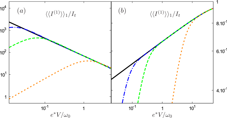
Figure 1: Single-qp backscattering current as a function of the external voltage $e^{{*}}V/\omega_{0}$, with $\omega_{0}=10^{-3}\omega_{c}$, in bilogarithmic scale for $\nu=2/5$ and topological neutral modes $\omega_{n}=0$. (a) Unrenormalized case $g_{c}=1$; (b) renormalized case $g_{c}=5.5$. Different line styles correspond to temperatures: $T/\omega_{0}=0$ (solid black), $0.025$ (dot-dashed blue), $0.1$ (dashed green), $2$ (short dashed orange). The unit of the current is $I_{t}=e|\mathsf{t}|^{2}/(4\pi^{2}a^{2}\omega_{c})$. The zero temperature power-laws of the figures are given by $V^{-4/5}$ and $V^{g_{c}/5-1}$ for the unrenormalized and the renormalized case respectively.

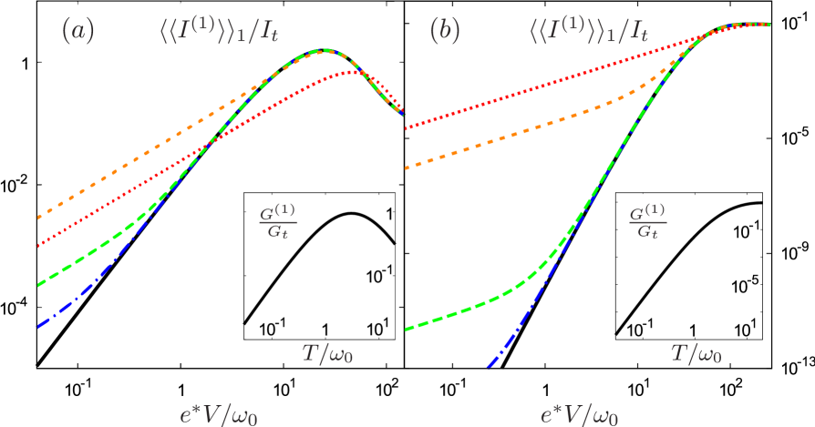
Figure 2: Single-qp backscattering current as a function of the external voltage $e^{{*}}V/\omega_{0}$, with $\omega_{0}=10^{-3}\omega_{c}$, in bilogarithmic scale for $\nu=2/5$ and propagating neutral modes with $\omega_{n}=10^{-2}\omega_{c}$. (a) Unrenormalized case $g_{c}=g_{n}=1$; (b) renormalized case $g_{c}=5.5$ and $g_{n}=2$. Different line styles correspond to temperatures: $T/\omega_{0}=0$ (solid black), $0.025$ (dot-dashed blue), $0.1$ (dashed green), $2$ (short dashed orange), $20$ (dotted red). At zero-temperature the power-laws scaling are: $V^{g_{c}/5+3g_{n}-1}$ for $e^{*}V\ll\omega_{n}$ and $V^{g_{c}/5-1}$ for $e^{*}V\gg\omega_{n}$. The unit for the current is as in figure 1. In the inset the linear conductance in unit of $G_{t}=e^{2}|\mathsf{t}|^{2}/(4\pi^{2}a^{2}\omega_{c}^{2})$ is represented in a bilogarithmic scale as a function of temperature.

Figure 1 shows the voltage dependence of the backscattering current for topological neutral mode ($\omega_{n}=0$) in the unrenormalized case $g_{c}=1$ panel (a) and in the renormalized case $g_{c}=5.5$ panel (b). At zero temperature, black lines, one recovers from (47) the power-law behaviour

$$\left\langle\left\langle I^{(1,top)}\right\rangle\right\rangle_{1}\propto V^{2\nu g_{c}\alpha_{1}^{2}-1},$$ (48)

driven by the charge exponent coefficient $\alpha_{1}$ and with a charge renormalization $g_{c}$. For the unrenormalized case figure 1(a) and for finite temperatures (coloured lines) the current exhibits a maximum around $e^{*}V\approx T$ with a linear ohmic behaviour for smaller voltages $e^{*}V\ll T$, and a power-law  (48) at higher bias $e^{*}V\gg T$.

For sufficiently strong charge renormalization $g_{c}>p^{2}/2\nu$ ($g_{c}>5$ for $\nu=2/5$), as shown in  1(b), the power-law exponent in (48) is positive and the current is always growing. Then, for finite temperatures the maximum is substituted by a smooth change of power-laws between the ohmic regime and the zero temperature behaviour (48).

We can now compare the above behaviour with propagating neutral modes as shown in figures 2(a) and 2(b). Let us start with the zero temperature case, here the current displays two different scaling

$$\left\langle\left\langle I^{(1)}\right\rangle\right\rangle_{1}\propto V^{2\nu g_{c}\alpha_{1}^{2}+2g_{n}\beta_{1}^{2}-1} e^{*}V\ll\omega_{n}$$ (49)

$$\left\langle\left\langle I^{(1)}\right\rangle\right\rangle_{1}\propto V^{2\nu g_{c}\alpha_{1}^{2}-1} e^{*}V\gg\omega_{n}$$ . (50)

Neutral modes contribute to the dynamics only for voltages smaller than the bandwidth $\omega_{n}$. The power-law exponent (49) is always positive because of (44) and $g_{c},g_{n}\geq 1$. Only at higher voltages $e^{*}V\gg\omega_{n}$, as in (50), one recovers the standard FL behaviour of the single-qp current where the dynamical contribution of neutral modes is absent (cf. (48)). For weak renormalization $g_{c}<p^{2}/2\nu$ ($g_{c}<5$ for $\nu=2/5$), as represented in figure 2(a), a maximum at $V=V^{0}_{\rm max}$ separates the two above regimes, while for strong renormalization $g_{c}>p^{2}/2\nu$ as in figure 2(b), the maximum is replaced by a smooth crossover at $V=V_{\rm c}^{0}$ with a growing current. The two quantities $V^{0}_{\rm max}$ and $V_{\rm c}^{0}$ are defined at zero temperature as their notation remind us. In general both $V^{0}_{\rm max}$ and $V_{\rm c}^{0}$ are proportional to $\omega_{n}$. However, their precise values depend on the parameters such as the filling factor and the renormalizations. For example, $V^{0}_{\rm max}$ can be obtained from (46), in the limit $\omega_{c}\to\infty$, by solving the equation

$$\ _{1}F_{1}\left[2g_{n}\beta^{2}_{1},2\nu g_{c}\alpha^{2}_{1}+2g_{n}\beta^{2}_{1}-1,-e^{*}V^{0}_{\rm max}/\omega_{n}\right]=0\,.$$ (51)

For $\nu=2/5$ and $g_{n}=g_{c}=1$, we find $\rme^{*}V^{0}_{\rm max}\approx 2.5\,\omega_{n}$ in accordance with the position of the maximum in figure 2(a).

At finite temperatures and low voltages $e^{*}V\ll T$ the current shows a linear behaviour $\left\langle\left\langle I^{(1)}\right\rangle\right\rangle_{1}\approx G^{(1)}V$ proportional to the linear conductance $G^{(1)}$. The latter is represented in the insets of the figure 2, at temperatures smaller than the neutral bandwidth, $T\ll\omega_{n}$, neutral modes affect its scaling with $G^{(1)}\propto T^{2(\nu g_{c}\alpha_{1}^{2}+g_{n}\beta_{1}^{2}-1)}$. On the other hand, at $T\gg\omega_{n}$ the scaling is driven by the charged mode only with $G^{(1)}\propto T^{2(\nu g_{c}\alpha_{1}^{2}-1)}$ [32]. These two power-laws are distinguishable in the curves presented in the insets.

At larger voltages the scaling behaviour (49) with neutral modes is still visible for voltages range $T/e^{*}\ll V\ll V^{0}_{\rm max}$ for weak renormalizations (figure 2(a)) or for $T/e^{*}\ll V\ll V^{0}_{\rm c}$ for the strong case (figure 2(b)). Under these conditions the maximum and the crossover position remain substantially uneffected varying the temperature. Only at higher temperatures $T/e^{*}\gtrsim V^{0}_{\rm max}$ or $T/e^{*}\gtrsim V^{0}_{\rm c}$, depending on the renormalization, the neutral modes are saturated at any voltages. Their dynamical contributions disappear and the current directly pass from the linear behaviour to the power-law (50) determined by the charged modes only. In these high temperatures condition, represented in figure 2 with orange and red lines, the position of the maximum $V_{\rm max}$ or the crossover $V_{\rm c}$ starts to increase linearly with temperature.

The above discussion shows two important aspects:

• renormalization effects change qualitatively the current behaviour;

• neutral modes dynamics may be visible in the current.

In particular, we have seen that weak interactions may be most favourable in order to achieve point ii). Indeed, the experimental verification of a temperature independent maximum position, which would be a trade-mark of the presence of neutral modes is more easily detectable than the measurement of a temperature independent crossover that would be the case for strong renormalization.

We would like to conclude by commenting that if it seems not too difficult to give evidence of the neutral modes, much more delicate is the possibility to quantitative determine the neutral bandwidth $\omega_{n}$, since the current behaviour depends crucially on other a priori unknown parameters.

4.2 Single-qps and $p$-agglomerates crossover phenomena

In this part we will consider the behaviour of the total backscattering current $\left\langle\left\langle I_{tot}\right\rangle\right\rangle_{1}$in  (43) given by the current contributions of the two most relevant processes: the single-qp $\left\langle\left\langle I^{(1)}\right\rangle\right\rangle_{1}$, and the $p$-agglomerate $\left\langle\left\langle I^{(p)}\right\rangle\right\rangle_{1}$. The aim will be to investigate the crossover phenomena among these two different terms. We remind that the weight of these tunnelling processes are given by $t_{1}\equiv\mathsf{t}$ and $|t_{p}|=\kappa_{p}|\mathsf{t}|$. In the following $\kappa_{p}$ will be assumed as a free parameter. Since the experimental data, such as [30], shows the presence of single-qp at larger voltages/temperatures and the presence of $p$-agglomerates only for lower energies one need to choose $\kappa_{p}$ sufficiently low such that the effects of the $p$-agglomerate are not visible at high energies but it has to be big enough to see them at sufficiently low energies.

In order to determine $\left\langle\left\langle I^{(p)}\right\rangle\right\rangle_{1}$ we remind that the most relevant $p$-agglomerate operator in (15) is given by $d=q=0$. This implies $\beta_{p}=0$ in (14), with no presence of neutral modes in the dynamics. Only charged modes will enter with the coefficient $\alpha_{p}=1$ as stated in (9). This allows to determine the current $\left\langle\left\langle I^{(p)}\right\rangle\right\rangle_{1}$ by using the results obtained in the previous section for the single-qp process with topological neutral modes $\omega_{n}=0$ - see (47) - apart from the necessary substitution $\alpha_{1}\to\alpha_{p}=1$.

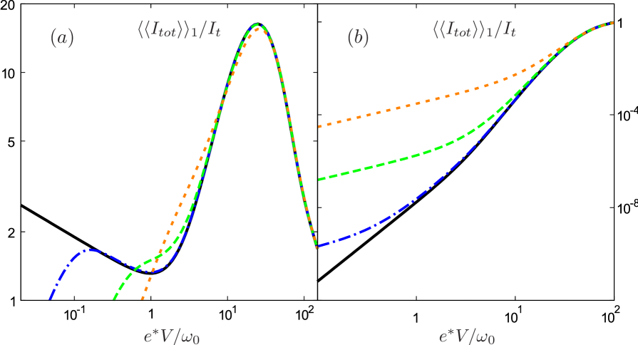
Figure 3: Total backscattering current $\left\langle\left\langle I_{tot}\right\rangle\right\rangle_{1}$ as a function of $e^{{*}}V/\omega_{0}$, with $\omega_{0}=10^{-3}\omega_{c}$, in bilogarithmic scale for $\nu=2/5$. (a) Unrenormalized case $g_{c}=g_{n}=1$ with $\kappa_{p}=0.4$; (b) renormalized case $g_{c}=5.5$ and $g_{n}=2$, with $\kappa_{p}=10$. Temperatures are $T/\omega_{0}=0$ (solid black), $0.025$ (dot-dashed blue), $0.1$ (dashed green), $2$ (short dashed orange). The neutral mode bandwidth is $\omega_{n}=10^{-2}\omega_{c}$. Unit of current: $I_{t}=e|\mathsf{t}|^{2}/(4\pi^{2}a^{2}\omega_{c})$.

Figures 3(a) and 3(b) show the total backscattering current as a function of voltage for unrenormalized and renormalized cases respectively, and $\nu=2/5$.

We start the discussion at zero temperature corresponding to black lines. The current shows three different power-laws

$$\left\langle\left\langle I_{tot}\right\rangle\right\rangle_{1}\propto V^{2\nu g_{c}\alpha_{p}^{2}-1} V\ll V^{*}$$ (52)

$$\left\langle\left\langle I_{tot}\right\rangle\right\rangle_{1}\propto V^{2\nu g_{c}\alpha_{1}^{2}+2g_{n}\beta_{1}^{2}-1}\, V^{*}\ll V\ll\omega_{n}/e^{*}$$ (53)

$$\left\langle\left\langle I_{tot}\right\rangle\right\rangle_{1}\propto V^{2\nu g_{c}\alpha_{1}^{2}-1} \omega_{n}/e^{*}\ll V$$ , (54)

with $\alpha_{p}$, $\alpha_{1}$ in (9) and $\beta_{1}$ in (44). Here, we defined with $V^{*}$ the bias at which the two main current contributions, at zero temperature, are equal $\left\langle\left\langle I^{(p)}\right\rangle\right\rangle_{1}=\left\langle\left\langle I^{(1)}\right\rangle\right\rangle_{1}$. The precise value of this point crucially depends on $\kappa_{p}$ and on other parameters.

Note that the power-laws (52)-(54) depend on the parameters $g_{c,n}$ which may affect qualitatively the behaviour. We already discuss their influence on the single-qp contribution, here we would like to focus mainly on the $p$-agglomerate part, which dominates the current at low voltages, see (52), and on the crossover region.

For weak values of charge renormalizations $1\leq g_{c}<1/2\nu$ the current decreases with voltages at $V<V^{*}$, see (52) and the black line in figure 3(a) present a minumum around $V^{*}$. This behaviour is completely different from the case of larger renormalizations $g_{c}>1/2\nu$, which shows an increasing current (cf. figure 3(b)). In this last case, there is a tendency to lose the clear evidence of the $p$-agglomerate which merges very smoothly on the single-qp contribution. Indeed, the crossover is only signalled by a change in the power-law that is gradually less evident increasing charge renormalization. Hence, we can conclude that, at $T=0$, the weak interaction case with $1\leq g_{c}<1/2\nu$, which exhibits a minimum in the current, is the most favourable in order to show the presence of $p$-agglomerates.

We would like now to investigate the robustness of the above results for finite temperature. The main task is to extract the voltage and temperature ranges where one could clearly detect the contribution of $p$-agglomerates. At finite temperatures (colored lines in figure 3 ), and low bias $V\ll T/pe^{*}<V^{*}$ the current, instead of the power-law (52), shows a linear behaviour typical of the ohmic regime preventing divergence at very low voltages for weak interactions ($g_{c}<1/2\nu$). On the other hand at larger voltages $T/pe^{*}\ll V<V^{*}$ it is possible to detect the presence of $p$-agglomerates from the behaviour of the current that follows the power-law  (52). At larger voltages $V\gg V^{*}$, single-qp dominates and current is similar to the $T=0$ cases (53) and (54).

As a common trend we observe that the optimal possibility to detect agglomerates depends crucially on the interaction parameters $g_{c,n}$. From figure 3(a), representative of weak renormalization $g_{c}<1/2\nu$, one can see that the transition between the linear behaviour to the $p$-agglomerates scaling can create a peak around $pe^{*}V\approx T$. In this case the current exhibits two peaks: the first due to the crossover between ohmic behaviour and the $p$-agglomerate power-law, the second due to the crossover inside the single-qp contribution due to the de-activation of neutral modes. Increasing interactions ( $g_{c}>1/2\nu$) the first peak tends to disappear until for strong enough interactions, $g_{c}>p^{2}/2\nu$, as in figure 3(b), even the second maximum disappears in accordance with the behaviour of the single-qp contribution discussed in the previous section. Here, the change in the power-law induced by the appearance/disappearance of $p$-agglomerates becomes less visible.

The above discussions demonstrate that is possible to find voltages and temperatures regimes where the agglomerate contributions are detectable in the current. In order to confirm this important result we would like to find stronger signatures in other transport properties. The study of higher current moments, performed in the next section, will represent a powerful tool to clarify the crossover physics between the $p$-agglomerates and single-qps.

4.3 Fano factor and higher cumulants

Noise measurements are important tools in order to obtain clear information on the carrier charges involved in transport and consequently on the dominant excitations present in the tunnelling current.

In order to study the current fluctuations we start by considering the Fano factor $F_{2}=\left\langle\left\langle I_{tot}\right\rangle\right\rangle_{2}/e|\left\langle\left\langle I_{tot}\right\rangle\right\rangle_{1}|$ defined as the ratio between the zero frequency noise of the total backscattering current and the current itself. Using (38) one can write the Fano in terms of single-qp and $p$-agglomerate current contributions

$$\hskip-14.22636ptF_{2}=\frac{e^{*}}{e}\frac{\left\langle\left\langle I^{(1)}\right\rangle\right\rangle_{1}\coth(\beta e^{*}V/2)+p\left\langle\left\langle I^{(p)}\right\rangle\right\rangle_{1}\coth(\beta pe^{*}V/2)}{|\left\langle\left\langle I^{(1)}\right\rangle\right\rangle_{1}+\left\langle\left\langle I^{(p)}\right\rangle\right\rangle_{1}|}\,.$$ (55)

In the following we will restrict the discussion at energies smaller than the neutral bandwidth, i.e. $e^{*}V,T\lesssim\omega_{n}$, for which crossover phenomena appear.

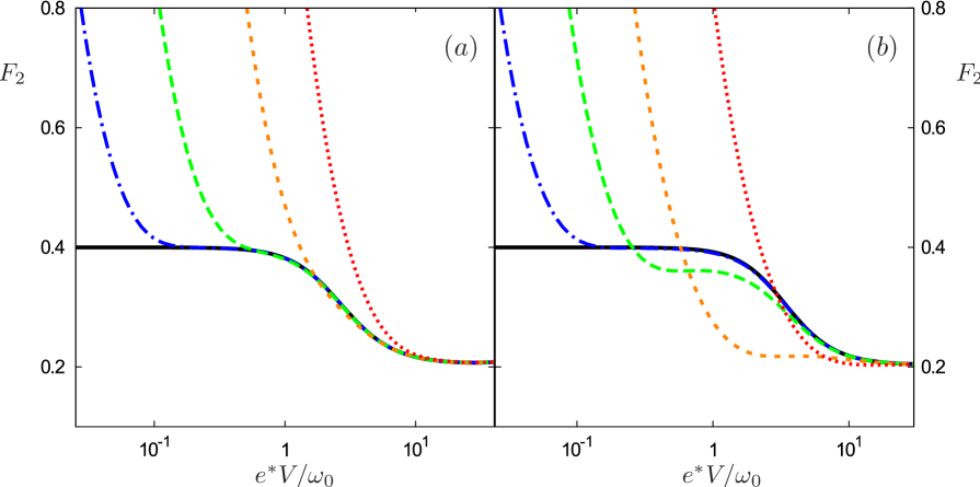
Figure 4: Fano factor $F_{2}$ as a function of bias $e^{*}V/\omega_{0}$, with $\omega_{0}=10^{-3}\omega_{c}$, in linear-logarithmic scale for $\nu=2/5$ and for $\omega_{n}=10^{-2}\omega_{c}$. (a) Unrenormalized case $g_{c}=g_{n}=1$, with $\kappa_{p}=0.4$; (b) renormalized case $g_{c}=5.5$ and $g_{n}=2$, with $\kappa_{p}=10$. Different line styles correspond to temperatures: $T/\omega_{0}=0$ (solid black), $0.025$ (dot-dashed blue), $0.1$ (dashed green), $0.5$ (short dashed orange), $2$ (dotted red).

Figure 4 shows the Fano factor as a function of bias at $\nu=2/5$ in the unrenormalized case, panel 4(a), and in the strong renormalized case, panel 4(b). At zero temperature (black lines) the system is in the shot-noise regime, from (55) one then has

$$F^{0}_{2}=\frac{e^{*}}{e}\frac{\left\langle\left\langle I^{(1)}\right\rangle\right\rangle_{1}+p\left\langle\left\langle I^{(p)}\right\rangle\right\rangle_{1}}{\left\langle\left\langle I^{(1)}\right\rangle\right\rangle_{1}+\left\langle\left\langle I^{(p)}\right\rangle\right\rangle_{1}}\,.$$ (56)

We remind that the total current in (52)-(54) is dominated by the $p$-agglomerates for $V\ll V^{*}$ where $\left\langle\left\langle I_{tot}\right\rangle\right\rangle_{1}\approx\left\langle\left\langle I^{(p)}\right\rangle\right\rangle_{1}$, and by the single-qp at $V\gg V^{*}$ where $\left\langle\left\langle I_{tot}\right\rangle\right\rangle_{1}\approx\left\langle\left\langle I^{(1)}\right\rangle\right\rangle_{1}$. Hence, the Fano shows two different plateaux

$$F^{0}_{2}\approx \frac{pe^{*}}{e}=\nu\, V\ll V^{*}$$ (57)

$$F^{0}_{2}\approx \frac{e^{*}}{e}=\frac{\nu}{p}\, V\gg V^{*}$$ . (58)

At low bias - cf. (57) - the Fano is dominated by $p$-agglomerates with effective charge $pe^{*}$, while at higher voltages - cf. (58) - the single-qp prevails with charge $e^{*}$. This behaviour is clearly showed in figures 4(a) and 4(b) and is stable against renormalization effects. Low and high bias regimes are separated by an interpolating region. As shown in [32] the width of this region is not universal and crucially depends on the interaction strength.

Note that the presence of two plateaux in the Fano is a direct evidence of the existence of two different kind of carriers that participate to tunnelling. At the zero temperature their charges are deduced by the values of the plateaux themselves.

In order to compare with experiments we need to generalize the above results at finite temperatures. We will see that some previous conclusions are still valid despite the presence of more intricate regimes. At small voltages $pe^{*}V\ll T$ the noise is represented by the Johnson-Nyquist thermal contribution with $F_{2}=2k_{B}T/eV$ and is diverging for $V\to 0$. This is clearly visible in all the finite temperature curves of figure 4. For the discussion at larger voltages we consider separately weak and strong renormalizations. Let us start with figure 4(a). For temperatures smaller than the threshold voltage $V^{*}$ and voltages in the range $T/pe^{*}\ll V<V^{*}$ the Fano reaches the first higher plateau at $F_{2}\approx\nu$ related to the charge of the $p$-agglomerate. On the other hand, at higher bias, it drops to the second plateau at $F_{2}\approx\nu/p$ corresponding to the charge of the single-qp.

At larger temperatures $T\gtrsim e^{*}V^{*}$ the visibility of the $p$-agglomerate is compromised by the presence of thermal noise. Indeed, the Fano directly passes from the Johnson-Nyquist regime to the single-qp plateau (see e.g. orange and red curves in figure 4(a)) without a possibility to detect the $p$-agglomerate plateau. One then can say that, for weak interaction one may detect the presence of two different excitations with a proper determination of charges only if $T\ll e^{*}V^{*}$, that typically in the experiments correspond to very low temperatures.

For strong renormalizations, as in figure 4(b), the results are even more involved. While the extremely low and high temperature regimes with $T\ll e^{*}V^{*}$ and $T\gg e^{*}V^{*}$ show a similar behaviour as observed above, at intermediate temperatures qualitatively differences appear. For example green line in figure 4(b) shows two plateaux, but the first is at an intermediate value $\nu/p\leq F_{2}^{*}\leq\nu$ smaller than the $p$-agglomerate charge. The origin of this behaviour is due to the smooth crossover between the $p$-agglomerate and the single-qp contributions present for strong interaction. Indeed, differently from the unrenormalized case, there is a finite region of bias where the two current contributions are comparable. Hence, the plateau value at $F_{2}^{*}$ corresponds to a weighted average of the single-qp $(e^{*}/e)$ and $p$-agglomerate $(pe^{*}/e)$.

We can then summarize the following important results:

• the existence of more than one plateau in the Fano factor is a clear trademark of the presence of more than one relevant tunnelling entity;

• whenever more than one relevant tunnelling process is simultaneously present is not appropriate to evaluate the effective charge involved in tunnelling by fitting the noise in (38) using a single carrier charge as free parameter.

This second procedure is often used in experiments [14, 15, 29, 30], however it could bring to misinterpretations. For example, in the above case with an intermediate plateau at $F_{2}^{*}$, the current is still composed by two different excitations with different charges equally important. In this case fitting the Fano with a single effective charge will give a wrong description. All these observations could be relevant for the experiment in [30] especially for $\nu=3/7$, where apparently the Fano factor instead to be equal to $3/7$, even at low temperatures, reaches only the value of $2.4/7$.

In this last part of the section we would like to generalize the above discussion considering higher current cumulants. In view of their statistical independence, we expect to obtain complementary information on carrier charges from them. We define the generalized Fano factors as the normalized $k$-th order zero frequency current cumulants [53]

$$F_{k}=\frac{\left\langle\left\langle I_{tot}\right\rangle\right\rangle_{k}}{e^{k-1}\left\langle\left\langle I_{tot}\right\rangle\right\rangle_{1}},$$ (59)

with $\left\langle\left\langle I_{tot}\right\rangle\right\rangle_{k}$ the total cumulant defined in (43). In the following we will consider the behaviour of odd cumulants with a detailed analysis of the normalized skewness $F_{3}$. This quantity is indeed experimentally accessible for a QPC in a Hall bar [47, 48]. The general expression for odd $k$-th normalized cumulants can be easily obtained inserting (42) and (43) in (59)

$$F_{k}=\left(\frac{e^{*}}{e}\right)^{k-1}\frac{\left\langle\left\langle I^{(1)}\right\rangle\right\rangle_{1}+(p)^{k-1}\left\langle\left\langle I^{(p)}\right\rangle\right\rangle_{1}}{\left\langle\left\langle I_{tot}\right\rangle\right\rangle_{1}}\ .$$ (60)

Note that this expression also holds at finite temperatures for odd $k$-th cumulant. For even $k$-th cumulants a $\coth(me^{*}V/T)$ term appears such that (60) is only valid at low temperatures $T\ll e^{*}V$. The absence of this term in the odd cumulants avoids divergences induced by the thermal regime which are, on the other hand, always present for even cumulants. Following similar analysis as done for the Fano we can extract the zero temperature behaviour of (60)

$$F^{(0)}_{k}\approx \left(\frac{pe^{*}}{e}\right)^{k-1}=\nu\,^{k-1}\, V\ll V^{*}$$ (61)

$$F^{(0)}_{k}\approx \left(\frac{e^{*}}{e}\right)^{k-1}=\left(\frac{\nu}{p}\right)^{k-1}\, V\gg V^{*}$$  . (62)

Again two plateaux appear with values related to the $p$-agglomerate charge at low voltages and to the single-qp charge at high voltages, with the power $(k-1)$. The skewness in figure 5 reproduce this behaviour (black lines) both for the unrenormalized case of figure 5(a) and for the strong renormalization of figure 5(b).

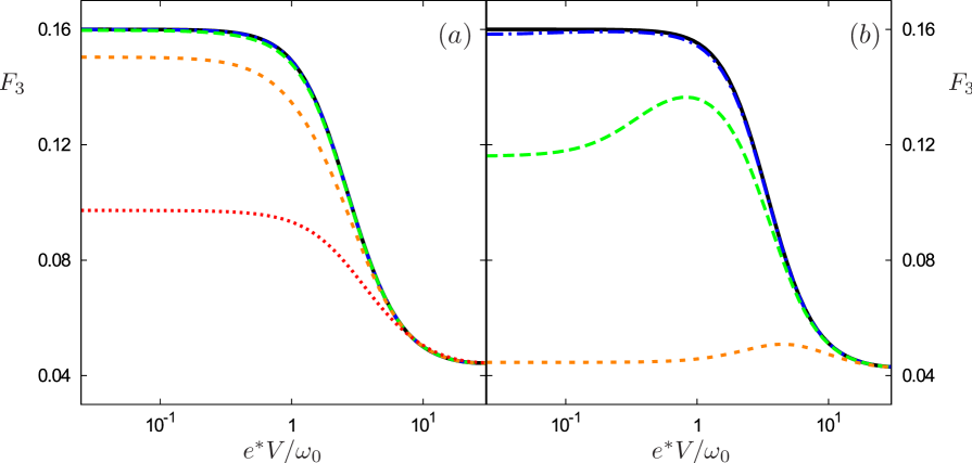
Figure 5: Normalized skewness $F_{3}$ as a function of bias $e^{*}V/\omega_{0}$, with $\omega_{0}=10^{-3}\omega_{c}$, in linear-logarithmic scale for $\nu=2/5$ and $\omega_{n}=10^{-2}\omega_{c}$. (a) Unrenormalized case $g_{c}=g_{n}=1$ with $\kappa_{p}=0.4$; (b) renormalized case $g_{c}=5.5$ and $g_{n}=2$ with $\kappa_{p}=10$. The different line styles correspond to different temperatures according the same convention adopted in figure 4. The units are the same as figure 4.

Increasing temperature the two plateaux are still present with a decrease of the higher with respect to the $T=0$ value. Note that the thermal divergence is not present here. Therefore, from the odd cumulants behaviour, one can have information on different excitations (looking at the different plateaux) even in the deep thermal regime $e^{*}V\ll T$ which is not an observable regime in noise measurements.

To be more specific let us compare the two red curves in figures 5(a) and 4(a). While for the Fano the thermal regime cancels out completely the presence of the higher plateau, this one is still clearly visible in the skewness. This means that odd moments can be an important tool in order to detect the presence of different excitations (e.g. the $p$-agglomerate and the single-qp in our case) present in tunnelling processes.

More delicate issue is the possibility to measure the precise values of the excitation charges. Indeed, as we saw before, one has to consider low enough temperatures (blue curves in figure 5) in order to measure, from the higher plateau, the value of the charge associated with the $p$-agglomerate. This can be explained by observing that for $V\to 0$, the current is proportional to the linear conductances (41), consequently, from (60) the cumulants are

$$F_{k}=\left(\frac{e^{*}}{e}\right)^{k-1}\frac{G^{(1)}+(p)^{k-1}G^{(p)}}{G^{(1)}+G^{(p)}}\,.$$ (63)

As extensively discussed in [32] one can verify that for temperatures low in comparison to the neutral modes bandwidth, $T\ll\omega_{n}$, the temperature power-law of the single-qp conductance is $G^{(1)}\propto T^{2[g_{c}\nu/p^{2}+(1+1/p)g_{n}-1]}$ with positive exponent, while for the $p$-agglomerate one has $G^{(p)}\propto T^{2(g_{c}\nu-1)}$ with an exponent that changes sign for $g_{c}>1/\nu$.

Therefore for weak renormalization, $g_{c}<1/\nu$, decreasing temperature, the $p$-agglomerate conductance strongly increase, and, at the same time, the single-qp contribution becomes negligible. Then one does not need extremely low temperatures in order to measure the true charge of $p$-agglomerate from the value of the plateau. This is well represented in figure 5(a) (green curve) where the skewness at low bias approaches the value $\nu^{2}$. Note that this charge would have been more difficult to be extracted from the Fano behaviour where the plateau is not so clearly defined - see the same curve in figure 4(a) -. For strong renormalization $g_{c}>1/\nu$, as in figure 5(b), the power-law exponents of the conductances $G^{(1)}$ and $G^{(p)}$ are both positives. Then, the dominance of the $p$-agglomerate appears at much lower temperatures with respect to the previous case and the plateau deviates from the $T=0$ value at temperatures lower than the weak renormalization case. In both case for temperatures not sufficiently low the intermediate values of the higher plateau depend on the weighted average of the two carrier contributions.

5 Conclusion

We investigated the effects of propagating neutral modes in the tunnelling of quasiparticles through a QPC for the Jain sequence of FQH. We observed that these modes qualitatively modify the behaviour of the single-qp backscattering current. Even more interesting they determine the behaviour of the total backscattering current given by the sum of the single-qp and the $p$-agglomerate contribution. We demonstrated that the presence of neutral modes with finite bandwidth creates a crossover between the two kinds of quasiparticles involved in tunnelling. To avoid non universal effects that may hide the possibility to extract information on this crossover we considered the current fluctuations. These quantities are indeed more robust than the current in order to identify unequivocally the entities which tunnel. We first investigated the Fano factor that presents a plateaux structure related to the crossover between the single-qp and the $p$-agglomerate tunnelling regime. However, the Fano is strongly affected by thermal effects, therefore, we considered odd higher cumulants. We demonstrated that higher cumulants are an important tool in order to establish the number of relevant quasiparticle in the tunnelling. This is a strong motivation for investigating these quantities, despite of the enormous technical difficulties in their measurements.

The cross-check of the physics described in this paper with some other independent transport quantities such as the finite frequency noise  [68, 78, 79] could open extremely interesting perspectives in the comprehension of anomalous behaviours that emerge in noise measurements. We are confident that analogous approaches could explain some unclear experimental observation for also the case $\nu=5/2$. [57, 80].

Appendix A

This Appendix is devoted to the derivation of the coefficients $\beta_{m}$ in (14). Let us start to discuss the monodromy condition introduced in section 2.1. The generalization of the internal statistical angle (6) for two different agglomerates with $m$ and $m^{\prime}$ is the so called mutual statistical angle $\Theta$ defined as [61]

$$\Psi^{(m)}(x)\Psi^{(m^{\prime})}(x^{\prime})=\Psi^{(m^{\prime})}(x^{\prime})\Psi^{(m)}(x)e^{-i\ \Theta\ \textrm{sgn}(x-x^{\prime})},$$ (64)

the phase depends on the coefficients $(\alpha,\beta(k))$ and $(\alpha^{\prime},\beta^{\prime}(k^{\prime}))$ that define two different operators in (8) with (see (9) and (10))

$$\alpha_{m}=\frac{m}{p}\,;\qquad\beta_{m}(k)=\sqrt{m^{2}\left(1+\frac{1}{p}\right)+2k},$$ (65)

and similar expressions for $\alpha_{m^{\prime}}$ and $\beta_{m^{\prime}}(k^{\prime})$. By using the operator commutation rules one obtains from (64)

$$\Theta[\alpha_{m},\beta_{m}(k);\alpha_{m^{\prime}},\beta_{m^{\prime}}(k^{\prime})]=\pi\left[\nu\alpha_{m}\alpha_{m^{\prime}}-\beta_{m}(k)\beta_{m^{\prime}}(k^{\prime})\right].$$ (66)

The monodromy condition imposes that the phase acquired by any excitations $m$ in a loop around an electron must be a multiple of $2\pi$ [62, 63]. We then need, first of all, to start the discussion considering the electron operator, which corresponds to $m=2p+1$. For this we will generalize the results presented in [61], where the $\nu=2/5$ case was discussed. In order to recover the electron operator of the original FL theory we consider $\beta_{2p+1}(k^{\prime})$ in (65) with $k^{\prime}=0$ [61], we will check at the end the admissibility of this value. Other electron operators in (64) with $k\not=0$ need to satisfy the mutual statistics constraint with the electron at $k^{\prime}=0$. From (66) it is

$$\Theta=\pi\left[\nu\alpha_{2p+1}\alpha_{2p+1}-\beta_{2p+1}(k)\beta_{2p+1}(0)\right]=\pi r$$ (67)

with $r\in\mathbb{Z}$. Inserting (65) in (67) one has

$$2+\frac{1}{p}-\left(2+\frac{1}{p}\right)\sqrt{(p+1)(4p^{3}+8p^{2}+5p+1+2kp)}=r.$$ (68)

To fulfil this equation one needs first of all to impose a constraint on the square root with

$$(p+1)(4p^{3}+8p^{2}+5p+1+2kp)=a^{2}.$$ (69)

Hence, the monodromy condition (68) can be written as

$$\frac{2p+1}{p}(1-a)=r.$$ (70)

One can see that to fulfil the two above equations one needs integer values of $a$. The more general solution of (70), is then written in terms of a number $u\in\mathbb{Z}$

$$a=1+up,\qquad r=-u(2p+1).$$ (71)

Replacing the above solution for $a$ in (69) one has

$$pu^{2}+2u-(4p^{3}+12p^{2}+13p+6)=2k(p+1).$$ (72)

This represents a parabolic Diophantine equation for $u$ and $k$. In the following, we will restrict the analysis to the case with $p\leq 6$. Here, the only possible solution, is given by

$$u=1+t(p+1),\qquad k=\frac{1}{2}(p+1)(t-2)(2+2p+pt),$$ (73)

where $t\in\mathbb{Z}$. For $p>6$ more complicated solutions are present and will be not discussed in this paper. Note that the $t=2$ value in (73) gives $k=0$, in accordance with the initial choice $k^{\prime}=0$ in (67). Replacing the expression (73) for $k$ in (65), with $m=2p+1$ we obtain

$$\alpha_{2p+1}=2+\frac{1}{p};\,\qquad\beta_{2p+1}(t)=\sqrt{p\left(p+1\right)}\left(t+\frac{1}{p}\right).$$ (74)

Now we generalize the analysis to the $m$-agglomerates. The monodromy condition (66) between an $m$-agglomerate described by (65) and an electron, described by (74) is

$$\frac{\Theta}{\pi}=\frac{m-\sqrt{2kp+m^{2}(p+1)}\sqrt{(p+1)}(pt+1)}{p}=v\,$$ (75)

where $v\in\mathbb{Z}$. Similarly to the previous case, one has first to impose a constraint on the square root (75)

$$\left[2kp+m^{2}(p+1)\right](p+1)=b^{2}.$$ (76)

The monodromy condition is then written as

$$\frac{m-b(1+pt)}{p}=v.$$ (77)

One can see that to fulfil the two above equations one first need integer values of $b$. The solution of (77) is then

$$b=m-fp,\qquad v=f+(fp-m)t\qquad(f\in\mathbb{Z}).$$ (78)

Replacing the above solution for $b$ in (76) one has to solve the relation

$$f^{2}p-2fm-m^{2}(p+2)=2k(p+1),$$ (79)

whose solution can be easily derived, again for $p\leq 6$,

$$f=-m-h(p+1),\qquad k=h(p+1)(m+\frac{h}{2}p)$$ (80)

with $k\in\mathbb{Z}$.

Note that for $m=2p+1$ and choosing $f=2-u$ one recover the equation (72) for the electron. Through the redefinitions $m=sp+d$ and $h=q-s$ $(q\in\mathrm{Z})$, we can rewrite (80) as

$$k=\frac{p\left(p+1\right)}{2}\left(q^{2}-s^{2}\right)+d\left(p+1\right)\left(q-s\right).$$ (81)

This corresponds to the expression (12) quoted in the main text. Replacing (81) in the initial expression (65) for $\beta_{m}(k)$ and using the notation $m=sp+d$ one has

$$\beta_{m}(q)=\sqrt{p\left(p+1\right)}\left(q+\frac{d}{p}\right)$$ (82)

as defined in (14). Note that for $s=2$, $d=1$ and with the trivial identification $q=t$ we recover the expressions for the electron in (74).

References

References

- [1] Laughlin R B 1983 Phys. Rev. Lett. 50 1395
- [2] Tsui D C, Stormer H L and Gossard A C 1982 Phys. Rev. Lett. 48 1559
- [3] Das Sarma S and Pinczuk A 1997 Perspective in quantum Hall effecs: novel quantum liquid in low-dimensional semiconductor structures (New York: Wiley)
- [4] Myrheim J 1999 Les Houches Session LXIX A. Comtet et. al. eds. (Berlin: Springler-Verlag)
- [5] Murthy G and Shankar R 2003 Rev. Mod. Phys. 75 1101
- [6] Stormer H L, Tsui D C and Gossard A C 1999 Rev. Mod. Phys. 71 S298
- [7] Moore J E 2009 Physics 2 82
- [8] Susskind L 1995 J. Math. Phys. 36 6377
- [9] Wen X G 1990 Phys. Rev. Lett. 64 2206
- [10] Wen X G 1991 Phys. Rev. B 43 11025
- [11] Wen X G 1990 Phys. Rev. B 41 12838
- [12] Kane C L and Fisher M P A 1994 Phys. Rev. Lett. 72 724
- [13] Chamon C de C, Freed D E and Wen X G 1996 Phys. Rev. B 53 4033
- [14] de Picciotto R, Reznikov M, Heiblum M, Umansky V, Bunin G and Mahalu D 1997 Nature 389 162
- [15] Saminadayar L, Glattli D C, Jin Y and Etienne B 1997 Phys. Rev. Lett. 79 2526
- [16] Camino F E, Zhou W and Goldman V J 2007 Phys. Rev. B 76 155305
- [17] Wilczek F 1990 Fractional Statistics and anyon Superconductivity (Singapore: World Scientific)
- [18] Jain J K 1989 Phys. Rev. Lett. 63 199
- [19] MacDonald A H 1990 Phys. Rev. Lett. 64 220
- [20] Wen X G and Zee A 1992 Phys. Rev. B 46 2290
- [21] Kane C L and Fisher M P A 1997 Phys. Rev. B 55 15832
- [22] Cappelli A, Huerta M and Zemba G R 2002 Nucl. Phys. B 636 568
- [23] Lopez A and Fradkin E 1999 Phys. Rev. B 59 15323
- [24] Grayson M, Tsui D C, Pfeiffer L N, West K W, and Chang A M 1998 Phys. Rev. Lett. 80 1062
- [25] Grayson M 2006 Solid State Commun. 140 66
- [26] Kane C L and Fisher M P A 1995 Phys. Rev. B 51 13449
- [27] Chang A M 2003 Rev. Mod. Phys. 75 1449
- [28] Chamon C, Fradkin E and Lopez A 2007 Phys. Rev. Lett. 98 176801
- [29] Reznikov M, de Picciotto R, Griffiths T G, Heiblum M and Umansky V 1999 Nature 399 238
- [30] Chung Y C, Heiblum M and Umansky V 2003 Phys. Rev. Lett. 91 216804
- [31] Heiblum M 2003 Physica E 20 89
- [32] Ferraro D, Braggio A, Merlo M, Magnoli N and Sassetti 2008 Phys. Rev. Lett. 101 166805
- [33] Fiete G A, Refael G and Fisher M P A 2007 Phys. Rev. Lett. 99 166805
- [34] Grosfeld E and Das S 2009 Phys. Rev. Lett. 102 106403
- [35] Levkivskyi I P and Sukhorukov E V 2008 Phys. Rev. B 78 045322
- [36] Levkivskyi I P, Boyarsky A, Fröhlich J and Sukhorukov E V 2009 Phys. Rev.B 80 045319
- [37] Wan X, Hu Z H, Rezayi E H and Yang K 2008 Phys. Rev. B 77 165316
- [38] Overbosch B J and Chamon C 2009 Phys. Rev. B 80 035319
- [39] Ilan R, Grosfeld E and Stern A 2008 Phys. Rev. Lett. 100 086803
- [40] Cappelli A, Georgiev L S and Zemba G R 2009 J. Phys. A 42 222001
- [41] Cappelli A, Viola G and Zemba G R 2009 Chiral partition function of quantum Hall droplet Preprint cond-mat/0909.3588v1
- [42] Rosenow B and Halperin B I 2002 Phys. Rev. Lett. 88 096404
- [43] K. Yang 2003 Phys. Rev. Lett. 91 036802
- [44] Jolad S and Jain J K 2009 Phys. Rev. Lett. 102 116801
- [45] Nazarov Yu V 2003 Quantum Noise in Mesoscopic Physics (Delft: Kluwer Academic Publishers)
- [46] Levitov L S and Reznikov M 2004 Phys. Rev. B 70 115305
- [47] Reulet B, Senzier J and Prober D E 2003 Phys. Rev. Lett. 91 196601
- [48] Bomze Y, Gershon G, Shovkun D, Levitov L S and Reznikov M 2005 Phys. Rev. Lett. 95 176601
- [49] Gustavsson S Leturcq R, Simovic B, Schleser R, Ihn T, Studerus P, Ensslin K, Driscoll D C and Gossard A C 2006 Phys. Rev. Lett. 96 076605
- [50] Fujisawa T, Hayashi T, Tomita R and Hirayama Y, Science 312 1634
- [51] Levitov L S and Lesovik G B 1993 JETP Lett 58 230
- [52] Levitov L S, Lee H and Lesovik G B 1996 J. Math. Phys. 37 4845
- [53] Braggio A, Merlo M, Magnoli N and Sassetti M 2006 Phys. Rev. B 74 041304
- [54] Griffiths T G, Comforti E, Heiblum H, Stern A and Umansky V 2000 Phys. Rev. Lett. 85 3918
- [55] Rodriguez V, Roche P, Glattli D C, Jinb Y and Etienne B 2002 Physica E 12 88
- [56] Heiblum M 2006 Physica Status Solidi (b) 243 3604
- [57] Dolev M, Heiblum M, Umansky V, Stern A and Mahalu D 2008 Nature 452 829
- [58] Geller M R and Loss D 1997 Phys. Rev. B 56 9692
- [59] Merlo M, Braggio A, Magnoli N and Sassetti M 2007 Phys. Rev. B 74 041304(R)
- [60] Fröhlich J and Zee A 1991 Nucl. Phys. B 364 517
- [61] Ferraro D, Braggio A, Magnoli N and Sassetti M 2009 Physica E doi:10.1016/j.physe.2009.06.037
- [62] Fröhlich J, Studer U M and Thiran E 1997 J. Stat. Phys. 86 821
- [63] Ino K 1998 Phys. Rev. Lett. 81 5908
- [64] Haldane F D M 1981 J. Phys. C 14 2585
- [65] Haldane F D M 1981 Phys. Rev. Lett. 47 1840
- [66] Guyon R, Devillard P, Martin T and Safi I 2002 Phys. Rev. B 65 153304
- [67] Martin T 2005 Les Houches Session LXXXI H. Bouchiat et. al. eds. (Amsterdam: Elsevier)
- [68] Chamon C, Freed D E and Wen X G 1995 Phys. Rev. B 51 2363
- [69] Weiss U 1999 Quantum dissipative system (Singapore: World scientific)
- [70] Papa E and MacDonald A H 2004 Phys. Rev. Lett. 93 126801
- [71] Mandal S S and Jain J K 2002 Phys. Rev. Lett. 89 096801
- [72] Palacios J J and MacDonald A H 1996 Phys. Rev. Lett. 76 118
- [73] Keldysh L V 1964 Zh. Eksp. Teor. Fiz. 47 1515
- [74] Kamenev A and Levchenko A 2009 Adv. Phys. 58 197
- [75] Mahan G D 1990 Many-particle physics (New York: Kluwer Academic Publishers Group)
- [76] Schottky W 1918 Ann. Phys. (Leipzig) 57 541
- [77] Kane C L and Fisher M P A 1992 Phys. Rev. Lett. 68 1220
- [78] Bena C and Safi I 2007 Phys. Rev B 76 125317
- [79] Zakka-Bajjani E, S gala J, Portier F, Roche P, Glattli D C, Cavanna A and Jin Y 2007 Phys. Rev. Lett. 99 236803
- [80] Willet R L, Pfeiffer L N and West K W 2009 PNAS 106 8853