Thermal flux of quasiparticles and the transition between two regimes of turbulence in ³He-B

Abstract

We compute the Andreev reflection coefficient of a flux of thermal quasiparticles in ³He-B incident upon various two-dimensional vortex configurations. We find that, for the same number of positive and negative vortex points, the reflection coefficient is much reduced if the points are arranged in pairs (which corresponds to a gas of vortex rings in three-dimensions) rather than random (which corresponds to a vortex tangle in three-dimensions). This results is consistent with measurements performed by Bradley et al. at the University of Lancaster.

Experimental and theoretical studies of turbulence in superfluid ⁴He and ³He have revealed features which are similar to what happens in the classical turbulence but also features which have no classical counterpart. The study of quantum turbulence at very low temperatures is particularly interesting because, in the absence of the normal fluid, the turbulence consists simply of a tangle of reconnecting, thin vortex filaments. Since all filaments have the same core radius and the same circulation, the problem of turbulence is reduced to the geometry and the topology of the tangle. Unfortunately, unlike what happens in the study of ordinary turbulence, only few methods of visualization are possible in liquid helium. In superfluid ³He-B, the Andreev scattering technique can be used to detect vortex filaments. This technique, pioneered at Lancaster, is based on the fact that the energy dispersion curve, $E=E({\bf p})$ of quasiparticles of momentum $\bf p$ is tied to the reference frame of the superfluid, so, in a superfluid moving with velocity ${\bf v}_{s}$, the dispersion curve becomes $E({\bf p})+{\bf p}\cdot{\bf v}_{s}$ (see the review article Fisher2008 ). Thus a side of a vortex line presents a potential barrier to oncoming quasiparticles, which can be reflected back almost exactly becoming quasiholes; the other side of the vortex lets the quasiparticles to go through. Quasiholes are reflected or transmitted in the opposite way. The vortex thus casts a symmetric shadow for quasiparticles at one side and for quasiholes at the other side Nugzar_1 , and, by measuring the flux of excitations, one detects the presence of the vortex.

However the extrapolation from the scattering of quasiparticles off one vortex to the scattering off many vortices may be nontrivial. In our earlier work Nugzar_2 we used a simplified 2-dimensional vortex point model, and found that the Andreev shadow caused by simple configurations of several point vortices is not necessarily equal to the sum of shadows of individual, isolated vortices (in the cited work such a phenomenon was called a ‘partial screening’). This result may have non-trivial implications for the interpretation of Andreev reflection measurements of the vortex line density in turbulent ³He-B.

The present work is motivated by the experimental observations of Bradley et al. BradleyPRL2005 of the transition from a gas of vortex rings to a dense vortex tangle. Still using the simplified 2-dimensional model, the question which we ask is whether a gas of vortex rings and a dense tangle have a different Andreev signature.

We start with describing the motion of vortices which, in the considered two-dimensional approximation, become vortex points. Such a two-dimensional system of point vortices in the inviscid fluid is known as the Onsager’s point vortex gas. Each vortex point moves with the flow field generated by all other vortices. In the $(x,\,y)$-plane, the $i^{\rm th}$ vortex point located at time $t$ at the position ${{\bf{r}}}_{i}(t)=x_{i}(t){\bf{i}}+y_{i}(t){\bf{j}}$, where ${\bf{i}}$ and ${\bf{j}}$ are, respectively, the unit vectors in the $x$- and $y$-directions, generates the fluid velocity field

$${{\bf{v}}}_{i}({{\bf{r}}},\,t)=\frac{\kappa_{i}}{2\pi|{{\bf{r}}}-{{\bf{r}}}_{i}|^{2}}[-(y-y_{i}){\bf{i}}+(x-x_{i}){\bf{j}}],$$ (1)

where $\kappa_{i}$ is the circulation generated by the $i^{\rm th}$ vortex. In the considered two-dimensional point vortex gas modelling turbulent ³He-B, $\kappa_{i}=\pm\kappa$ with $\kappa=\pi\hbar/m\approx 0.662\times 10^{-3}~{}\textrm{cm}^{2}/\textrm{s}$, where $\kappa$ is the quantum of circulation in ³He-B, $m$ is the mass of ³He atom, and the signs plus and minus denote respectively a vortex generating the anticlockwise rotation of the fluid in the $(x,\,y)$-plane, and an antivortex generating the clockwise rotation. At the point ${\bf{r}}$, the velocity field created by the system of $N$ vortices is given by the superposition of the velocity fields generated by all vortices.

An isolated pair of a vortex and an antivortex can be considered as a two-dimensional model of a three-dimensional vortex ring. Such a pair moves through the fluid, in the direction orthogonal to the line connecting the vortex and the antivortex, with the velocity $V=\kappa/(2\pi d)$, where $d$ is the distance between the vortex points in this pair. Obviously, in the point vortex gas a vortex and an antivortex can be considered a pair (a 2D vortex ring) if $d$ is much smaller than the average distance between the center of this pair and the nearest vortex which does not belong to this pair.

To model turbulence in ³He-B, we consider the following three configurations of the vortex points:

$1^{\rm o}$. A spatially random system of $N$ point vortices of the same polarity; such a system has net circulation $|\kappa_{t}|=N\kappa$. This configuration can be considered as the two-dimensional model of a polarized vortex bundle Alamri .

$2^{\rm o}$. A random, statistically uniform system of $N/2$ vortices and $N/2$ antivortices in the case where the distance between any two vortex points is not much smaller than $L/\sqrt{N}$, where $L$ is the size of the computational domain, so that vortices and antivortices are not organized in pairs. In such a system there is no net circulation, $\kappa_{t}=0$. This configuration can be considered as a two-dimensional model of a vortex tangle.

$3^{\rm o}$. A system of vortex-antivortex pairs such that the distance $d$ between the vortex points in each pair is the same, but locations and orientations of pairs are random. This configuration can be considered the two-dimensional model of a gas of vortex rings.

The configurations $2^{\rm o}$ and $3^{\rm o}$ can be characterized by two geometric quantities, $d$ and the average distance, say $a$ between the centers of two neighbouring vortex-antivortex pairs. The relevant non-dimensional parameter characterizing the configuration is $\zeta=d/a\leq 1$. Gas of small, compared to the mean intervortex distance, vortex-antivortex pairs (configuration $3^{\rm o}$) corresponds to $\zeta\ll 1$. Of particular interest is the transition between configurations $3^{\rm o}$ and $2^{\rm o}$. Such a transition corresponds, in a modelling sense, to the experimental observations of Bradley et al. BradleyPRL2005 of the transition from the gas of vortex rings to the dense vortex tangle. In the considered two-dimensional system of vortex points this transition can be modelled by increasing the parameter $\zeta$ from small values corresponding to $d$ of the order of $100\xi_{0}$, where $\xi_{0}\approx 0.85\times 10^{-5}\,{\rm cm}$ is the zero-temperature coherence length, to values of the order of unity.

We consider the two-dimensional problem of ballistic propagation of quasiparticle excitations in the flow field of the point vortex gas and the gas of vortex-antivortex pairs described by configurations $1^{\rm o}$, $2^{\rm o}$, and $3^{\rm o}$. Neglecting spatial variations of the order parameter, in the presence of the flow field the energy of thermal excitation can be written as

$$E=\sqrt{{\mbox{$\epsilon_{p}$}}^{2}+\Delta_{0}^{2}}+{\bf{p}}\cdot{\bf{v}}_{s}({\bf{r}},\,t),$$ (2)

where ${\mbox{$\epsilon_{p}$}}=p^{2}/(2m^{*})-{\mbox{$\epsilon_{F}$}}$ is the kinetic energy of a thermal excitation of momentum ${\bf{p}}$ relative to the Fermi energy ${\mbox{$\epsilon_{F}$}}\approx 2.27\times 10^{-16}~{}\rm erg$ (here and below the numerical values are taken at zero bar pressure Wheatley ), $m^{*}\approx 3.01m=1.51\times 10^{-23}~{}\rm g$, with $m$ being the mass of the ³He atom, and $\Delta_{0}=1.76k_{B}T_{c}\approx 2.43\times 10^{-19}~{}\rm erg$, with $k_{B}$ being the Boltzmann’s constant and $T_{c}$ the critical temperature, is the superfluid energy gap. (It should be noted that the superfluid energy gap was assumed a constant value, $\Delta_{0}$. because we are concerned with the behaviour of thermal excitation at distances $r$ from the vortex core larger than the zero-temperature coherence length $\xi_{0}$.) Excitations with ${\mbox{$\epsilon_{p}$}}>0$ are called quasiparticles, and excitations with ${\mbox{$\epsilon_{p}$}}<0$ are called quasiholes.

Following the approach of Refs. Nugzar_1 ; Nugzar_2 we assume that the interaction term ${\bf{p}}\cdot{\bf{v}}_{s}$ varies on a spatial scale which is larger than $\xi_{0}$ so that the excitation can be regarded as a compact object of momentum ${\bf{p}}={\bf{p}}(t)$, position ${\bf{r}}={\bf{r}}(t)$, and energy $E=E({\bf{p}},\,{\bf{r}},\,t)$ given by Eq. (2). Using the method developed in Refs. Leggett ; Yip , Eq. (2) can be considered as an effective, semi-classical Hamiltonian yielding the following equations of motion:

$$\dot{{\bf{r}}}=\frac{\partial E({\bf{p}},\,{\bf{r}},\,t)}{\partial{\bf{p}}}=\frac{{\mbox{$\epsilon_{p}$}}}{\sqrt{{\mbox{$\epsilon_{p}$}}^{2}+\Delta_{0}^{2}}}\frac{{\bf{p}}}{m^{*}}+{\bf{v}}_{s}({\bf{r}},\,t),$$ (3)

$$\dot{{\bf{p}}}=-\frac{\partial E({\bf{p}},\,{\bf{r}}\,t)}{\partial{\bf{r}}}=-\frac{\partial}{\partial{\bf{r}}}[{\bf{p}}\cdot{\bf{v}}_{s}({\bf{r}},\,t)].$$ (4)

Introducing the non-dimensional variables Nugzar_2

$${\bf{R}}=\frac{{\bf{r}}}{\xi_{0}},\,{\bf{V}}_{s}=\frac{\xi_{0}}{\kappa}{\bf{v}}_{s},\,\tau=\frac{t}{t_{0}},\,{\bf\Pi}=\frac{{\bf{p}}}{{\mbox{$p_{F}$}}},\,H=\frac{E}{\Delta_{0}},$$ (5)

where ${\bf{R}}=(X,\,Y)$, ${\mbox{$p_{F}$}}=\sqrt{2m^{*}{\mbox{$\epsilon_{p}$}}}\approx 8.28\times 10^{-20}~{}\rm g~{}cm/s$ is the Fermi momentum, and $t_{0}=\xi_{0}{\mbox{$p_{F}$}}/\Delta_{0}\approx 2.9\times 10^{-6}\,{\rm s}$, in the non-dimensional form the Hamiltonian (2) and the equations of motion (3)-(4) become

$$H=\sqrt{\lambda^{2}({\Pi}^{2}-1)^{2}+1}+m^{*}m^{-1}\pi^{2}{\bf\Pi}\cdot{\bf{V}}_{s}({\bf{R}},\,\tau),$$ (6)

and

$$\dot{\bf{R}}=\frac{2\lambda(\Pi^{2}-1)}{\sqrt{(\Pi^{2}-1)^{2}+\lambda^{-2}}}{\bf\Pi}+\frac{m^{*}}{m}\pi^{2}{\bf{V}}_{s}({\bf{R}},\,\tau),$$ (7)

$$\dot{\bf\Pi}=-m^{*}m^{-1}\pi^{2}{\mbox{\boldmath$\nabla$}}({\bf\Pi}\cdot{\bf{V}}_{s}({\bf{R}},\,\tau)),$$ (8)

where now $\dot{A}\equiv dA/d\tau$, and we introduced the non-dimensional parameter $\lambda={\mbox{$\epsilon_{F}$}}/\Delta_{0}$. In the following calculations we assume $\lambda=10^{3}$.

We solve numerically the equations (7)-(8) of ballistic motion of quasiparticles in order to calculate the propagation of thermal flux, generated by the point source of thermal excitations, through the point vortex gas configurations $1^{\rm o}$, $2^{\rm o}$, and $3^{\rm o}$ introduced above. The numerical method is described in our earlier work Nugzar_2 .

In turbulence experiments in ³He-B, the properties of the vortex tangle or the gas of vortex rings can be studied by measuring the heat which is transported by thermal excitations through the velocity field of the vortices Bradley-PRL2004 (see also the review article Ref. Fisher2008 ). A net flux of excitations (and, hence, energy) results in the case where there is a (small) temperature gradient. In this case the heat carried by excitations generated by the source (and, therefore, incident on the vortex gas) is

$$\delta Q_{inc}=\int_{\Delta_{0}}^{\infty}N_{F}{\mbox{$v_{F}$}}E\frac{\partial f(E)}{\partial T}\delta T\,dE,$$ (9)

where $\delta T\ll T$ is a temperature difference between the source of thermal excitations and the opposite side of the system, $N_{F}=m\sqrt{2m^{*}{\mbox{$\epsilon_{F}$}}}/(\pi^{2}\hbar^{3})$ is the density of states at the Fermi energy, ${\mbox{$v_{F}$}}={\mbox{$p_{F}$}}/m^{*}\approx 5.48\times 10^{3}\,{\rm cm/s}$ is the Fermi velocity, and $f(E)$ is the Fermi distribution, which, at the ultra low temperatures, becomes the Boltzmann distribution $f(E)=\exp(-E/k_{B}T)$.

In the case of an isolated vortex, one side of it presents a potential barrier to oncoming quasiparticles, which are Andreev reflected as quasiholes almost exactly back to the source. In our previous work Nugzar_1 we found that the Andreev shadow, i.e. the maximum distance from the vortex core past which a quasiparticle with the kinetic energy $\epsilon_{p}$ is not Andreev reflected, is $S_{0}=3\pi(\Delta_{0}/{\mbox{$\epsilon_{p}$}})^{2}$ in our dimensionless units. In the subsequent work Nugzar_2 it was shown that, due to partial screening, the Andreev shadow of simple configurations of several vortices is not necessarily equal to the sum of shadows of isolated vortices. Hence we have reasons to expect that in a gas of point vortices or in a gas of vortex-antivortex pairs (modelling, respectively, a vortex tangle or a gas of vortex rings) partial screening will strongly affect the heat flux carried back to the source by Andreev reflected quasiparticles.

The numerical simulation of the heat flux reflected by the point vortex gas was carried out in the rectangular domain. At $t=0$ the vortices are randomly distributed within the square sub domain whose non-dimensional coordinates are $-5\times 10^{3}\leq X\leq 5\times 10^{3}$, $-5\times 10^{3}\leq Y\leq 5\times 10^{3}$ (the size of this domain corresponds to the experimental estimates BradleyPRL2005 ; Fisher2001 ; Bradley-PRL2004 ; Bradley-PRL2006 ). The heat source is located at $(-1\times 10^{4},\,0)$ so that the angle, $\varphi$ between the $X$-axis and the beam of quasiparticles varies between $-\pi/4$ and $\pi/4$. The flux generated by the source is modelled by $K=25000$ quasiparticles whose non-dimensional initial energies, $H_{0}$ ($1\leq H_{0}\leq 1.688$) and directions, $\varphi_{0}$ are uniformly distributed. Since the source of excitations is located sufficiently far from the vortices, the initial momentum of quasiparticle whose initial energy is $H_{0}$ was calculated from Eq. (6) as $\Pi_{0}=[\lambda^{-1}(H_{0}^{2}-1)^{1/2}+1]^{1/2}$. For the Boltzmann distribution, $f(E)$, introducing $\tilde{E}=E/k_{B}T$ the integrand in (9) reduces to the $\Gamma(3)$ distribution which, in our numerical calculations, was generated by the standard subroutine and the resulting values were discarded if $\tilde{E}<\Delta_{0}/k_{B}T$. In the typical low temperature experiments, $\Delta_{0}/(k_{B}T)\approx 10$; this value was used throughout all calculations.

A trajectory of each quasiparticle was found by numerical solution of Eqs. (7)-(8) for random initial energies (momenta) and directions of motion. Having identified the trajectories of quasiparticles that are Andreev reflected (as quasiholes) by the vortex gas or a gas of vortex-antivortex pairs, for a particular realization, R of the initial configuration of the vortex gas the reflection coefficient is then calculated as

$$f_{r}^{\rm R}=\frac{1}{q_{0}}\sum_{j=1}^{K}\alpha_{i}H_{i0}\quad{\rm with}\quad q_{0}=\sum_{j=1}^{K}H_{i0},$$ (10)

where $\alpha_{j}=1$ if the $j^{\rm th}$ quasiparticle is reflected, otherwise $\alpha_{j}=0$, and $K=2.5\times 10^{4}$. This procedure has been carried out for $N_{\rm R}$ realizations of the initial configuration of the vortex gas, and the ensemble average reflection coefficient was calculated as $f_{r}=\langle f_{r}^{\rm R}\rangle$ for configurations $1^{\rm o}$, $2^{\rm o}$, and $3^{\rm o}$. Since the error of ensemble averaging decreases with the number of realizations as $N_{\rm R}^{-1/2}$, to achieve a reasonable (few per cent) accuracy we used up to $N_{\rm R}=2.5\times 10^{4}$ realizations.

At this point it seems useful to show a zoomed view of each of these configurations, see Fig. 1.

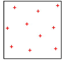
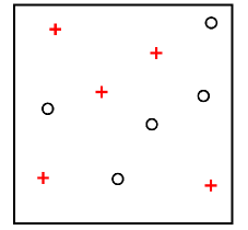
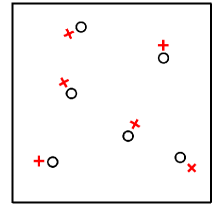
Figure 1: (Color online) Zoomed view of configurations $1^{\rm o}$ (left), $2^{\rm o}$ (center), and $3^{\rm o}$ (right); + (red) – vortices, ${\bf{\bigcirc}}$ (black) – antivortices.

Fig. 2 shows the reflection coefficient, $f_{r}$ as

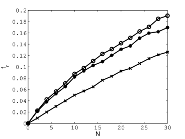
Figure 2: Reflection coefficient as a function of the total number of vortex points. Lines, from top to bottom, correspond to configurations $1^{\rm o}$, $2^{\rm o}$, and the gas of vortex-antivortex pairs $3^{\rm o}$ with $d=100\xi_{0}$.

a function of the total number of vortices, $N$ in the system. As can be seen from this figure, in all cases the reflection coefficient increases with the total density of the vortex points. The reflection coefficients in the system $1^{\rm o}$ of vortices of the same polarity and in the vortex gas $2^{\rm o}$ with zero net circulation are close, although in the latter case the partial screening seems to have a slightly bigger effect. However, in the case where the vortices of opposite polarities form pairs (‘rings’), partial screening plays a far more pronounced rôle and the reflection coefficient falls by almost an order of magnitude (in the calculation illustrated by the bottom line of Fig. 2 the dimensional distance between the vortex points in each pair was assumed $d=100\xi_{0}$).

As was already mentioned above, of particular interest is a behaviour of the reflection coefficient during the transition between configurations $2^{\rm o}$ and $3^{\rm o}$. Such a behaviour can be characterized by the reflection coefficient, $f_{r}$ as a function of the non-dimensional parameter $\zeta$. This function is illustrated by Fig. 3 for $N=26$ (for other

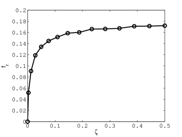
Figure 3: Reflection coefficient, for 13 vortex-antivortex pairs ($N=26$), as a function $\zeta=d/a$, where $d$ is the distance between the vortex and antivortex in a pair, and $a$ is the average distance between the centers of nearest pairs.

values of $N$ the behaviour of $f_{r}$ with $\zeta$ remains qualitatively the same). As can be seen, in the considered example, with 13 vortex-antivortex pairs, the increase of $\zeta=d/a$ from $\zeta=0.01$ (gas of small vortex-antivortex pairs) to $\zeta=0.2$ (almost random, disordered point vortex gas) is accompanied by almost five-fold increase of the reflection coefficient, from $f_{r}\approx 3.5\times 10^{-2}$ to 0.158, respectively, the latter value being not very different from that for the random point vortex gas ($f_{r}\approx 0.169$). Therefore, the results shown in Fig. 3 seem to indicate that the transition, observed by Bradley et al. BradleyPRL2005 , from the gas of vortex rings to the relatively dense vortex tangle can be detected by the significant (nearly an order of magnitude) increase of the coefficient of reflection of the heat flux carried by thermal excitations.

The experiment BradleyPRL2005 was performed at temperature $T=0.16~{}T_{c}$ and pressure $P\approx 0~{}{\rm bar}$ where $T_{c}$ is the critical temperature. Quantized vortices were generated by an oscillating grid and detected by two vibrating wires placed near the grid. A beam of quasiparticles illuminated the grid. In the presence of vortices a fraction of the quasiparticles is Andreev reflected, reducing the damping of the vibrating wire; this damping is caused by the asymmetry of the quasiparticles and quasiholes incident upon the wire. The transient response of the fractional change of the damping was measured as a function of the velocity of the oscillating grid. It was found that at high grid velocity ($4.5$ to $7.8~{}\rm mm/s$) the fractional reduction of damping was from $0.25$ to $0.4$ and recovered slowly in $10$ to $15~{}\rm s$, whereas at small grid velocity ($1.9$ to $2.9~{}\rm mm/s$) the fractional reduction of damping ranged from $0.025$ to $0.1$ and recovered quickly in less than $1~{}\rm s$. The experimenters suggested an interpretation based on the recovery time, i.e. that at high grid velocity quantum turbulence is created which slowly decay and disperse away. On the contrary, at small grid velocity the vorticity is in the form of a gas of vortex rings no larger than $5~{}\rm\mu m$, which quickly move away (the translational velocity of a vortex ring is inversely proportional to its size). Our computed results are consistent with this interpretation: we found that the reflection coefficient of a gas of vortex-antivortex points (the two-dimensional equivalent of a gas of vortex rings) is much less than that of a random vortex gas (the two-dimensional equivalent of a vortex tangle), which agrees with the experimental observation.

We are grateful to D. I. Bradley, G. R. Pickett, S. N. Fisher, W. F. Vinen, and also to the participants of the Workshop on Topics in Quantum Turbulence (Abdus Salam International Centre for Theoretical Physics, Trieste, March 2009) for stimulating discussions.

References

- (1) S. N. Fisher, in Vortices and Turbulence at Very Low Temperatures, edited by C. F. Barenghi and Y. A. Sergeev, CISM Courses and Lectures, Vol. 501 (Springer, Wien New York, 2008), pp. 177-257.
- (2) C. F. Barenghi, Y. A. Sergeev, and N. Suramlishvili, Phys. Rev. B 77, 104512 (2008).
- (3) C. F. Barenghi, Y. A. Sergeev, N. Suramlishvili, and P. J. van Dijk, Phys. Rev. B 79, 024508 (2009).
- (4) D. I. Bradley, D. O. Clubb, S. N. Fisher, A. M. Guénault, R. P. Haley, C. J. Matthews, G. R. Pickett, V. Tsepelin, and K. Zaki, Phys. Rev. Lett. 95, 035302 (2005).
- (5) S. Z. Alamri, A. J. Youd, and C. F. Barenghi, Phys. Rev. Lett. 101, 215302 (2008).
- (6) J.C. Wheatley, Rev. Mod. Phys. 47, 415 (1975).
- (7) N. A. Greaves and A. J. Leggett, J. Phys. C (Solid State Physics) 16, 4383 (1983).
- (8) S. Yip, Phys. Rev. B 32, 2915 (1985).
- (9) D. I. Bradley, S. N. Fisher, A. M. Guénault, M. R. Lowe, G. R. Pickett, A. Rahm, and R. C. V. Whitehead, Phys. Rev. Lett. 93, 235302 (2004).
- (10) S. N. Fisher, A. J. Hale, A. M. Guénault, and G. R. Pickett, Phys. Rev. Lett. 86, 244 (2001).
- (11) D. I. Bradley, D. O. Clubb, S. N. Fisher, A. M. Guénault, R. P. Haley, C. J. Matthews, G. R. Pickett, V. Tsepelin, and K. Zaki, Phys. Rev. Lett. 96, 035301 (2006)