Optical Precursors with Self-induced Transparency

Abstract

Optical Sommerfeld-Brillouin precursors significantly ahead of a main field of comparable amplitude have been recently observed in an opaque medium with an electromagnetically induced transparency window [Wei et al., Phys. Rev. Lett. 103, 093602 (2009)]. We theoretically analyze in this paper the somewhat similar results obtained when the transparency is induced by the propagating field itself and we establish an approximate analytic expression of the time-delay of the main-field arrival, which fits fairly well the result obtained by numerically solving the Maxwell-Bloch equations.

More than one century ago, Sommerfeld examined the apparent inconsistency between the existence of superluminal group velocities and the theory of relativity. Considering an incident field switched on at time $t=0$ (step pulse), he showed that, no matter the value of the group velocity, no field can be transmitted by a linear dispersive medium before the instant $t=L/c$ where $L$ is the medium thickness and $c$ the velocity of light in vacuum som07 . Subsequently he and Brillouin studied the fast oscillatory transients appearing at $t\geq L/c$ in the particular case of a single-resonance Lorentz medium som14 (2, 3). They named them forerunners insofar as, in proper conditions, they can distinctly precede the establishment of the steady-state field (the main field). Renamed optical precursors, forerunners have entered classical textbooks stra41 (4, 5) and continue to raise a considerable interest. The theoretical results of Sommerfeld and Brillouin have been improved, even rectified (the amplitude of the precursors was in particular strongly underestimated in their work), and different models of linear dispersive media have been considered. See oug07 (6) for a recent review.

Despite the abundant literature on precursors, there are very few papers reporting direct observation of precursors distinguishable from the main field. The difficulty of such an observation has been soundly discussed by Aavikssoo et al. aa88 (7) who achieved in 1991 an experiment involving single-sided exponential pulses (instead of step-pulses) and exploiting the dispersion originating from a narrow exciton line in AsGa aa91 (8). For proper detuning of the optical carrier frequency $\omega_{c}$ from the resonance frequency $\omega_{0}$, optical precursors appear as a small spike superimposed on the main pulse. See also jeon06 (9, 10). The observation of precursors significantly ahead of a main field of comparable amplitude obviously requires the use of long enough square pulses and of a medium fairly transparent at the optical carrier frequency, the corresponding group delay being long compared to the duration of the precursors. As discussed in jeon09 (11, 12), the latter conditions are met in an opaque medium with a narrow transparency window (slow light medium). Such an experiment has been recently achieved by Wei et al. wei09 (13) in an opaque cloud of cold atoms with an electromagnetically induced transparency (EIT) window. Note that, in this experiment (as in all the studies of precursors), the propagating field linearly interacts with the medium.

For comparison, we will examine here the nonlinear situation where the medium transparency is induced by the propagating field itself mcc69 (14, 15). Figure 1 shows the result of an experiment achieved in such conditions bs90 (16). The medium is a gas of $\mathrm{HC^{15}N}$ at low pressure contained in a 182m-long oversized waveguide and the incident wave is on resonance with the molecular rotational line $J=0,\,M=0\rightarrow J=1,\,M=0$ (wavelength $\lambda_{c}\approx 3.5$ mm). The gas behaves as a 2-level medium all87 (17) characterized by $T_{1}$ ($T_{2}$ ) the relaxation time for the population difference (the polarization), $T_{2}^{*}$ the Doppler time and $\alpha$ the resonant absorption coefficient at low intensity (extrapolated from the Lorentzian wings of the line). See bs89 (18) for details. The incident wave is characterized by $I_{0}$ its intensity normalized to the saturation intensity and $\tau_{r}$ its rise time. The observed step responses clearly have some similarities with those obtained in the EIT experiment wei09 (13), with a short transient preceding the establishment of a steady state regime (main field). The quasi Rabi oscillations crisp72 (15) accompanying the latter are obviously absent in the EIT experiments but oscillations having a linear origin (postcursors) can also be observed in this case bm09 (12).

Figure 1: Observed step response of a resonant absorbing medium. Parameters : $\alpha L\approx 200$ , $T_{1}\approx T_{2}\approx 10\>\mu\mathrm{s}$ ($T_{2}/\alpha L\approx 50\>\mathrm{ns}$), $T_{2}^{*}\approx 1.3\>\mu\mathrm{s}$ , $\omega_{c}=5.4\times 10^{11}\mathrm{s}^{-1}$ ($\omega_{c}^{-1}\approx 1.8\>\mathrm{ps}$ ), $\tau_{r}=12\>\mathrm{ns}$ ; $I_{0}\approx$ (a) 2100,(b) 960 (c) 620 (d) 350. In each case, the intensity is normalized to that of the step transmitted in the absence of gas (dashed line).

To analyze the previous results, we provisionally neglect the Doppler broadening and assimilate the guided wave to a plane wave propagating in the $z$ direction ($0<z<L$), with an electric field polarized in the $x$ direction. As long as $\tau_{r},\,T_{1},\,T_{2}\gg 1/\omega_{c}$ and $\alpha\ll\omega_{c}/c$, the slowly varying envelope approximation (SVEA) all87 (17) holds re1 (19) and we write the $E_{x}$ component of the electric field as :

$$E_{x}(z,t)=\mathrm{Re}\left[\mathrm{e}^{i\omega_{c}t}\widetilde{E}(z,t)\right]$$ (1)

where, as in all the following, $t$ is a local time (real time minus $z/c$), and $\widetilde{E}(z,t)$ is the slowly varying field envelope. Denoting $\mu$ the dipole matrix element for the transition (chosen real), $R(z,t)=\mu\widetilde{E}(z,t)/\hbar$ the Rabi frequency, $n(z,t)$ the population difference per volume unit ($n_{0}$ its value at equilibrium) and $\widetilde{P}(z,t)$ the envelope of the electric polarization induced in the medium, it is convenient to introduce the dimensionless quantities $D=n/n_{0}$, $P=\frac{i\widetilde{P}}{n_{0}\mu}\sqrt{\frac{T_{1}}{T_{2}}}$ and $E=\mu\widetilde{E}\sqrt{T_{1}T_{2}}/\hbar=R\sqrt{T_{1}T_{2}}$, all real in the resonant case. $I=E^{2}$ is the intensity normalized to the saturation intensity. The Maxwell-Bloch (MB) equations governing the system evolution take then the simple form

$$\frac{\partial E}{\partial z}=-\frac{\alpha}{2}P$$ (2)

$$T_{2}\frac{\partial P}{\partial t}=DE-P$$ (3)

$$T_{1}\frac{\partial D}{\partial t}=-PE+(1-D)$$ (4)

We assume that the rise time $\tau_{r}$ of the incident intensity, while long compared to $1/\omega_{c}$ (as above mentioned), is short with respect to all the other characteristic times of the system ($1/R$, $T_{1}$, $T_{2}$ and $T_{2}/\alpha L$). The response $E(L,t)$ of the medium (with a time resolution equal to $\tau_{r}$) is then obtained by solving the MB equations with $P(z,0)=0$, $D(z,0)=1$ and $E(0,t)=E_{0}\Theta(t)=\sqrt{I_{0}}\Theta(t)$ where $\Theta(t)$ is the unit step function. This problem has been examined by Crisp crisp72 (15) when the relaxation effects are negligible, a condition obviously not met in the experiments.

The long term behavior of the step response ($t\gg T_{1},T_{2}$ ) is obtained by solving the MB equations in steady state. Combining Eqs.3 and 4, we find $P=E/(1+E^{2})$ and, putting this result in Eq.2, we easily retrieve the transmission equation sel67 (20, 21, 22)

$$I(\infty)+\ln I(\infty)=I_{0}+\ln I_{0}-\alpha L$$ (5)

where $I(t)$ is a short hand notation of the transmitted intensity $I(L,t)$. The medium being optically thick in the linear regime ($\alpha L\gg 1$), the absorption is fully saturated ($I(\infty)/I_{0}\approx 1$) only when the incident (normalized) intensity is extremely large ($I_{0}\gg\alpha L$). In fact the transmitted field (main field) will be significant (partial transparency) as soon as $I_{0}-\alpha L=\mathrm{O}(\alpha L)$. The transmission equation takes then the approximate form $I(\infty)/I_{0}\approx 1-\alpha L/I_{0}$ and a transmission $I(\infty)/I_{0}>1/3$ is obtained for $I_{0}>3\alpha L/2$.

Consider now the short term behavior of the step response. By combining the integral form of Eqs.3 and 4 and taking into account that $D(z,t)\leq 1$, one can establish the inequality crisp70 (23)

$$1-D(z,t)<\left|\int_{0}^{t}R(z,t^{\prime})dt^{\prime}\right|^{2}<R_{0}^{2}t^{2}$$ (6)

where $R_{0}$ is the Rabi frequency associated with the incident step ( $R_{0}^{2}=\frac{I_{0}}{T_{1}T_{2}}$). When $R_{0}^{2}t^{2}\ll 1$, $D(z,t)\approx 1$ and the MB equations are reduced to the couple of linear equations $\partial E/\partial z=-\alpha P/2$ and $T_{2}\partial P/\partial t=E-P$. So, at least in this time domain and though $I_{0}\gg 1$, the medium behaves as a linear system (small pulse-area approximation crisp70 (23)). Its response $E(L,t)$ is easily retrieved from the previous couple of equations and can be written as lau78 (24, 25)

$$E(L,t)=E_{0}\Theta(t)\left(1-\alpha L\intop_{0}^{t/T_{2}}\frac{\mathrm{J}_{1}\left(\sqrt{2\alpha Lu}\right)}{\sqrt{2\alpha Lu}}\mathrm{e}^{-u}du\right)$$ (7)

When $\alpha L\gg 1$, the integral can be transformed to obtain

$$E(L,t)\approx E_{0}\Theta(t)\mathrm{e}^{-t/T_{2}}\mathrm{J}_{0}\left(\sqrt{2\alpha Lt/T_{2}}\right)$$ (8)

For $x>1$, $\mathrm{J}_{0}(x)\approx\sqrt{\frac{2}{\pi x}}\cos\left(x-\frac{\pi}{4}\right)$ and $E(L,t>\frac{T_{2}}{2\alpha L})\approx E_{+}(t)+E_{-}(t)$ where

$$E_{\pm}(t)=\frac{E_{0}}{\sqrt{2\pi}}\mathrm{e}^{-t/T_{2}}\frac{\exp\left[\pm i\left(\sqrt{2\alpha Lt/T_{2}}-\pi/4\right)\right]}{\left(2\alpha Lt/T_{2}\right)^{1/4}}$$ (9)

So the optical field is made of two components of equal amplitude and instantaneous frequency $\omega_{c}\pm\sqrt{\frac{\alpha L}{2tT_{2}}}$, which are nothing but that the Sommerfeld ($E_{+}$) and Brillouin ($E_{-}$) precursors as determined by the saddle point method of integration lef09 (26, 12, 27). The linear character of the short-term response (and thus its analysis in terms of precursors) is well supported by the experiments. As shown Fig.1, the shape of the corresponding transient is roughly independent of the incident intensity. By numerically solving the MB equations, we find that the condition $R_{0}^{2}t^{2}\ll 1$ is much too severe and that the linear approximation satisfactorily holds up to $t=2\pi/R_{0}$, the Rabi period of the incident field. It even holds later in the experiments because the transversal inhomogeneity of the field partially washes out the (nonlinear) quasi Rabi oscillations while it does not affect the linear response (the precursors).

In the EIT experiments, the probe field linearly interacts with the medium at every time and the arrival of the main field is determined by the (slow) group velocity bm09 (12). In the present case, this arrival is fixed by fully nonlinear phenomena, the study of which requires the resolution of the complete MB equations. We first examine the solution obtained in the rate equations approximation (REA) all87 (17). The equations to solve are then reduced to $\partial I/\partial z=-\alpha ID$ and $T_{1}\partial D/\partial t=-D((1+I)+1$ sel67 (20, 22) with $D(z,0)=1$ and $I(0,t)=I_{0}\Theta(t)$. Eliminating $D$ and integrating in $z$, we get bm08 (22)

$$T_{1}d\left(\ln I\right)/dt=\ln I_{0}+I_{0}-\alpha L-\ln I-I$$ (10)

with $I(0)=I_{0}\exp\left(-\alpha L\right)$. The transmitted intensity $I(t)$ is finally given by the implicit equation

$$\frac{t}{T_{1}}=\intop_{I_{0}\exp\left(-\alpha L\right)}^{I(t)}\frac{dI^{\prime}}{I^{\prime}\left(\ln I_{0}+I_{0}-\alpha L-\ln I^{\prime}-I^{\prime}\right)}$$ (11)

The transmission $T(t)=I(t)/I_{0}$ monotonously increases from $\exp\left(-\alpha L\right)$ to $I(\infty)/I_{0}$, where $I(\infty)$ is given by Eq.5. In the conditions considered here [$\alpha L\gg 1$, $I_{0}-\alpha L=\mathrm{O}(\alpha L)$], $T(0)\approx 0$, $T(\infty)\approx 1-\alpha L/I_{0}$ and the transition between these two values is very steep (Fig.2). The time-delay of the arrival of the main intensity is conveniently defined as the time $\tau_{d}$ such that $I(\tau_{d})=I(\infty)/2$. It is given by Eq.11 by taking $I(\infty)/2$ as upper limit of integration. When $I_{0}\gg\alpha L$ (full saturation limit), Eq.11 can be explicitly integrated to give $T(t)\approx\left[1+\exp\left(\alpha L-I_{0}t/T_{1}\right)\right]^{-1}$ in agreement with the result given in kry70 (28). The 10-90% rise time $\Delta t$ of the intensity and the time-delay $\tau_{d}$ then read as $\Delta t\approx 4\ln 3\left(T_{1}/I_{0}\right)$ and $\tau_{d}\approx\alpha L\left(T_{1}/I_{0}\right)\ll T_{1}$. When the saturation is only partial, the time-delay $\tau_{d}$ as a function of $1/I_{0}$ increases much faster than $\alpha LT_{1}/I_{0}$ and values of the order of $T_{1}$ can be attained while keeping a significant transmission (Fig.2).

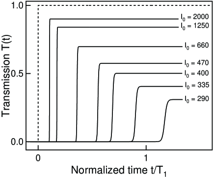
Figure 2: Step response obtained in the rate equations approximation (REA) as a function of the normalized time $t/T_{1}$. Optical thickness $\alpha L=200$. Each step response is labeled by the corresponding incident intensity $I_{0}$. The step response obtained for $I_{0}\rightarrow\infty$ is given for reference (dashed line).

The REA does not take into account the coherent effects. It eliminates in particular the quasi Rabi oscillations accompanying the main field. One may however expect that the signals obtained by this way are a satisfactory approximation of the exact signals, the oscillatory parts of which would have been filtered out. To check this idea, we have compared, $\alpha L$ and $I_{0}$ being fixed, the step response obtained by using the REA (independent of $T_{2}$) to those obtained by numerically solving the MB equations for two different values of $T_{2}/T_{1}$ (Fig.3).

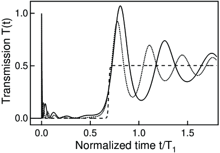
Figure 3: Comparison of the step response obtained by the REA (dashed line) to those obtained by numerically solving the Maxwell-Bloch (MB) equations with $T_{2}/T_{1}=1$ (full line) and with $T_{2}/T_{1}=1/2$ (dotted line). Other parameters: $\alpha L=200$ and $I_{0}=400$, leading to $T(\infty)\approx 1/2$. Note that the pseudo-period of the oscillations superimposed to the steady state in the MB solutions are nearly equal to the corresponding Rabi period $2\pi/R_{\infty}=2\pi\sqrt{T_{1}T_{2}/I(\infty)}$, namely $0.44T_{1}$ ($0.31T_{1}$) for $T_{2}/T_{1}=1$ ($T_{2}/T_{1}=1/2$).

The three step responses are obviously different but the time-delays $\tau_{d}$ (as defined before) are very close. Similar simulations made for different values of the parameters show that this result is not accidental. It appears that Eq.11 provides the exact time-delay with a precision better than $10\%$ in all the cases of physical interest, that is when the precursors are well developed before the arrival of the main field and the latter has a significant amplitude.

Figure 4: Numerical solution of the MB equations taking into account the transverse distribution of the field (full line) for $\alpha L=200$, $I_{0}=400$, and $T_{2}=T_{1}$. The REA (dashed line) and MB (dotted line) solutions obtained with the plane wave model are given for reference.

We will now examine the modifications brought to the step response by some effects neglected in the previous theoretical analysis. The most important one results from the transverse inhomogeneity of the guided wave. Figure 4 shows a typical step-response obtained by using a MB numerical code extended to include a transverse variation of the field pes91 (29). As expected, the linear part of the response (precursors) is not changed (it is even slightly prolonged) but the quasi Rabi oscillations (strongly depending on the field amplitude) are dramatically affected. Their amplitude is considerably reduced and their damping is accelerated, in agreement with the experimental result (Fig.1). However we remark that the time-delay $\tau_{d}$ is not significantly larger than that obtained in the plane-wave and rate-equations approximations. Similar calculations including the Doppler broadening instead of the field inhomogeneity in the plane-wave MB numerical code show that, even when $T_{2}^{*}=0.13T_{2}$ (parameters of Fig.1), the Doppler effect negligibly affects the precursors and slightly reduces the time-delay $\tau_{d}$. This can be explained by observing that the right time scale for the precursors and the nonlinear response is not $T_{2}$ but, respectively, $T_{2}/\alpha L\ll T_{2}^{*}$ and $1/R_{0}<T_{2}^{*}$. Finally, the finite rise time of the incident step essentially affects the most rapidly varying part of the step response, namely the transient associated with the precursors and first the intensity $I_{1}$ of its first peak. When $\alpha L\gg 1$, $I_{1}$ only depends on $r=\alpha L\tau_{r}/T_{2}$ and attains the intensity $I_{0}$ of the incident wave when $r\ll 1$. This condition is approximately met in the experiment reported in bs90 (16) where $I_{1}\approx 0.9I_{0}$ (Fig.1). Similar results could be obtained at optical wavelength by propagating a Gaussian beam in an ensemble of laser cooled 2-level atoms. We have then $T_{2}^{*}\gg T_{2}$ and the Doppler effect negligibly affects the precursors and the quasi Rabi oscillations. In other respects, $T_{2}$ (typically $50$ns) is about $200$ times shorter than in the microwave experiment. For a good observation of the precursors, the rise time of the incident step should also be $200$ times shorter, namely in the $50$ps range (attained with electro-optic modulators).

To summarize, we have shown that the experiments involving self-induced transparency are a good alternative to the EIT experiments in order to observe optical precursors well ahead of the main field, both having intensities comparable to that of the step-modulated incident wave. By using a plane-wave model and the rate equations approximation, we have established an analytical expression for the time-delay of the main-field arrival, which generalizes that previously obtained in the infinite saturation limit, and we have shown that this expression provides a good estimate of the real time-delay as long as precursors and main field are well separated and of significant amplitude.

References

- (1) A. Sommerfeld, Physikalische Zeitschrift 23, 841 (1907).
- (2) A. Sommerfeld, Ann. Phys. (Leipzig) 44, 177 (1914).
- (3) L. Brillouin, Ann. Phys. (Leipzig) 44, 204 (1914).
- (4) J.A. Stratton, Electromagnetic Theory (McGraw-Hill, New York 1941)
- (5) J.D. Jackson, Classical Electrodynamics, 2nd ed. (Wiley, New York 1975).
- (6) K.E. Oughstun, Electromagnetic and Optical Pulse Propagation 1 (Springer, Berlin 2007), Ch.1.
- (7) J. Aaviksoo, J. Lippman and J. Kuhl, J. Opt. Soc. Am. B 5, 1631 (1988).
- (8) J. Aaviksoo, J. Kuhl, and K. Ploog, Phys. Rev. A 44, R5353 (1991).
- (9) H. Jeong, A. M. C. Dawes, and D.J. Gauthier, Phys. Rev. Lett., 96, 143901 (2006).
- (10) S. Du, C. Belthangady, P. Kolchin, G.Y. Yin, and S.E. Harris, Opt. Lett. 33, 2149 (2008)
- (11) H. Jeong and S. Du, Phys. Rev. A 79, 011802(R) (2009).
- (12) B. Macke and B. Ségard, Phys. Rev. A 80, 011803(R) (2009).
- (13) Dong Wei, J.F. Chen, M.M.T. Loy, G.K.L. Wong, and S. Du, Phys. Rev. Lett. 103, 093602 (2009).
- (14) S.L. McCall and E.L. Hahn, Phys. Rev. 183, 457 (1969).
- (15) M.D. Crisp, Phys. Rev. A 5, 1365 (1972).
- (16) B. Ségard, B. Macke, J. Zemmouri, and W. Sergent, Ann. Phys. (Paris), Colloque n°1, Supplément au n°2, Vol.15 (1990), p.167.
- (17) L. Allen and J.H. Eberly, Optical resonance and two-level atoms (Dover, New York 1987).
- (18) B. Ségard, B. Macke, L.A. Lugiato, F. Prati, and M. Brambilla, Phys. Rev. A 39, 703 (1989).
- (19) These conditions are met in all the experiments having led to a direct observation of precursors.
- (20) A. Selden, Br. J. Appl. Phys. 3, 1935 (1967).
- (21) L.W. Hillman, R.W. Boyd, J. Krasinski, and C.R. Stroud, Opt. Commun. 45, 416 (1983].
- (22) B. Macke and B. Ségard, Phys. Rev. A 78, 013817 (2008).
- (23) M.D. Crisp, Phys. Rev. A 1, 1604 (1970).
- (24) A. Laubereau and W. Kaiser, Rev. Mod. Phys. 50, 607 (1978).
- (25) B. Ségard, J. Zemmouri, and B. Macke, Europhys. Lett. 4, 47 (1987).
- (26) W.R. LeFew, S. Venakides, and D.J. Gauthier, Phys. Rev. A 79, 063842 (2009).
- (27) This asymptotic method of integration is sometimes opposed to the SVEA. In fact it can pertinently be used in the frame of the latter bm09 (12).
- (28) P.G. Kryukov and V.S. Letokhov, Sov. Phys. Uspekhi 12, 641 (1970).
- (29) E.M. Pessina, B. Ségard, and B. Macke, Optics Commun. 81, 397 (1991).