Dual Quantization for random walks with application to credit derivatives

Abstract

We propose a new Quantization algorithm for the approximation of inhomogeneous random walks, which are the key terms for the valuation of CDO-tranches in latent factor models. This approach is based on a dual quantization operator which posses an intrinsic stationarity and therefore automatically leads to a second order error bound for the weak approximation. We illustrate the numerical performance of our methods in case of the approximation of the conditional tranche function of synthetic CDO products and draw comparisons to the approximations achieved by the saddlepoint method and Stein’s method.

Keywords: Quantization, Backward Dynamic programming, Random Walks.

1 Introduction

In this paper we focus on the numerical approximation of inhomogeneous Bernoulli random walks.

Therefore, let $(\Omega,\mathcal{F},(\mathcal{F}_{t}),\mathbb{P})$ be a filtered probability space on which we define the inhomogeneous random walk

$$X:=\sum_{i=1}^{n}\alpha_{i}Z_{i},$$ (1)

for some independent $\{0,1\}$-valued Bernoulli random variables $Z_{i}\sim\mathcal{B}(p_{i}),\,p_{i}\in(0,1)$ and $\alpha_{i}>0$.

The distribution of $X$ plays a crucial role for the valuation of basket credit derivatives like CDO-tranches in latent factor models (see e.g. [1] or [5]). These are credit products, whose payoff is determined by the loss in large portfolios of defaultable credit underlyings.

Therefore assume that we have a portfolio of $n$ defaultable credit names with notional amounts $N_{i}$ and whose default times $\tau_{i}$ are $(\mathcal{F}_{t})$ stopping times, $i=1,\ldots,n$. Here, $(\mathcal{F}_{t})$ stands for the observable filtration of the credit names. Moreover, we denote the fractional recovery of the $i$-th credit by $R_{i}$.

Hence, the fractional loss of the portfolio up to time $t$ is given by

$$l_{t}:=\sum_{i=1}^{n}\frac{(1-R_{i})N_{i}}{N}\mathbbm{1}_{\{\tau_{i}\leq t\}},$$ (2)

where $N=\sum_{i=1}^{n}N_{j}$ is the total notional.

Following the ideas of [6] and [3], the distributions of the default events $\{\tau_{i}\leq t\}$ up to a fixed time $t$ are driven under the risk-neutral probability measure by a common factor $U$ (which we may assume w.l.o.g. as $\mathcal{U}([0,1])$ distributed) and some idiosyncratic noise $\varepsilon_{i}$.

That means, that we assume that the events $\{\tau_{i}\leq t\},\,i=1,\ldots,n$ are conditionally independent given $\sigma(U)$.

Furthermore, we require the existence of a copula function $F:[0,1]^{2}\to[0,1]$, such that $p\mapsto F(p,u)$ is a non-decreasing, right continuous function for every $u\in[0,1]$ and

$$\int_{0}^{1}F(p,u)\,du=p,\quad p\in[0,1].$$

Since it holds

$$\begin{split}\mathbb{P}\bigl{(}\{\tau_{i}\leq t\}\bigr{)}=\mathbb{E}\bigl{(}\mathbb{P}(\{\tau_{i}\leq t\}|U)\bigr{)}&=\int_{0}^{1}\mathbb{P}\bigl{(}\{\tau_{i}\leq t\}|U=u\bigr{)}\,du\\ &=\int_{0}^{1}F\Bigl{(}\mathbb{P}\bigl{(}\{\tau_{i}\leq t\}\bigr{)}\,,u\Bigr{)}\,du,\end{split}$$

we may interpret $F\bigl{(}\mathbb{P}\bigl{(}\{\tau_{i}\leq t\}\bigr{)}\,,u\bigr{)}$ as the conditional default probability $\mathbb{P}(\{\tau_{i}\leq t\}|U=u)$.

Typical choices for the function $F$ are the standard Gaussian copula

$$F(p,u)=\Phi\left\{\frac{\Phi^{-1}(p)-\rho\Phi^{-1}(u)}{\sqrt{1-\rho^{2}}}\right\}$$

with common correlation parameter $\rho$, or the Clayton copula (cf. [5]).

Thus, for a fixed time $t$, the risk-neutral conditional distributions of the portfolio losses $l_{t}$ given the event $\{U=u\}$ are driven by a random walk of type (1) with $\alpha_{i}:=(1-R_{i})N_{i}/N$ and conditionally independent Bernoulli random variables $Z_{i}:=\mathbbm{1}_{\{\tau_{i}\leq t\}}$ with parameters $p_{i}:=F\Bigl{(}\mathbb{P}\bigl{(}\{\tau_{i}\leq t\}\bigr{)}\,,u\Bigr{)}$.

The cash flows of a (synthetic) CDO single tranche $[a,b]$ with attachment points $0\leq a<b\leq 1$ read as follows:

The protections seller of the tranche $[a,b]$ has to pay at each default time $\tau_{i}$ which satisfies $l_{\tau_{i}}\in[a,b]$ the notional of the defaulted name minus its recovery, i.e.

$$(1-R_{i})N_{i}.$$ (default leg)

On the other hand he continuously receives a coupon payment of

$$\kappa N_{l}^{[a,b]}(t)\,dt,$$ (premium leg)

where $\kappa$ is the fair spread of the tranche, which is to be determined by arbitrage arguments. We denote by $N_{l}^{[a,b]}(t)$ the outstanding notional of the tranche at time $t$, that is the notional amount of the tranche $[a,b]$ which has not defaulted up to time $t$ .

Assuming a deterministic risk-free interest rate $r$ and continuously compounding, we note that

$$\frac{(1-R_{i})N_{i}}{N}\mathbbm{1}_{[a,b]}(l_{\tau_{i}})=F_{l}^{[a,b]}(\tau_{i})-F_{l}^{[a,b]}(\tau_{i}-),$$

where the tranche losses $F_{l}^{[a,b]}$ are defined as

$$F_{l}^{[a,b]}(t):=(l_{t}-a)^{+}-(l_{t}-b)^{+}=\begin{cases}0&\text{if}\quad l_{t}<a\\ l_{t}-a&\text{if}\quad a\leq l_{t}\leq b\\ b-a&\text{if}\quad l_{t}>b\end{cases}.$$

Hence, the discounted default payments accumulated up to maturity $T$ maybe written as

$$\begin{split}\sum_{i=1}^{n}e^{-r\tau_{i}}(1-R_{i})N_{i}\mathbbm{1}_{[a,b]}(l_{\tau_{i}})&=N\sum_{i=1}^{n}e^{-r\tau_{i}}\bigl{[}F_{l}^{[a,b]}(\tau_{i})-F_{l}^{[a,b]}(\tau_{i}-)\bigr{]}\mathbbm{1}_{\tau_{i}\leq T}\\ &=N\int_{0}^{T}e^{-rt}F_{l}^{[a,b]}(dt).\end{split}$$

Concerning the premium leg, the outstanding notional $N_{l}^{[a,b]}(t)$ of the tranche $[a,b]$ is given by

$$N_{l}^{[a,b]}(t)=N\cdot\bigl{[}(b-a)-F_{l}^{[a,b]}(t)\bigr{]}=\begin{cases}N\cdot(b-a)&\text{if}\quad l_{t}<a,\\ N\cdot(b-l_{t})&\text{if}\quad a\leq l_{t}\leq b,\\ 0&\text{if}\quad l_{t}>b\end{cases}$$

so that the discounted coupon payments $\kappa\,e^{-rt}N_{l}^{[a,b]}(t)\,dt$ accumulate between $0$ and $T$ to

$$\kappa\cdot N\int_{0}^{T}e^{-rt}\bigl{[}(b-a)-F_{l}^{[a,b]}(t)\bigr{]}dt.$$

Under the risk-neutral probability measure both legs have to produce an equal present value, i.e.

$$N\int_{0}^{T}e^{-rt}F_{l}^{[a,b]}(dt)=\kappa\cdot N\int_{0}^{T}e^{-rt}\bigl{[}(b-a)-F_{l}^{[a,b]}(t)\bigr{]}dt,$$

so that taking (risk-neutral) expectation and processing an integration by parts yield the fair spread value $\kappa$, namely

$$\kappa=\frac{e^{-rt}\mathbb{E}F_{l}^{[a,b]}(T)+r\int_{0}^{T}e^{-rt}\mathbb{E}F_{l}^{[a,b]}(t)\,dt}{\frac{b-a}{r}\bigl{[}1-e^{-rT}]-\int_{0}^{T}e^{-rt}\mathbb{E}F_{l}^{[a,b]}(t)\,dt}.$$

Here, the mathematical challenge consists in the computation of the expectations $\mathbb{E}F_{l}^{[a,b]}(t)$. This leads, within the latent factor models, to the approximation of the conditional expectations

$$\mathbb{E}(F_{l}^{[a,b]}(t)|U=u)=\mathbb{E}((l_{t}-a)^{+}|U=u)-\mathbb{E}((l_{t}-b)^{+}|U=u),$$

since we have

$$\mathbb{E}F_{l}^{[a,b]}(t)=\int_{0}^{1}\mathbb{E}(F_{l}^{[a,b]}(t)|U=u)\,du.$$ (3)

As already announced, the conditional distribution of $l_{t}$ is given by an inhomogeneous random walk as defined in (1).

We therefore focus in this paper on the approximation of the distribution of this type of random walks, the outer integral with respect to $U$ in (3) can afterwards be approximated by standard quadrature formulae.

For the usual applications $n$ has a size of about 100, which is by far too large for an exact computation of the distribution of the random walk $X$, but still too small to get accurate approximations based on the asymptotics provided by limit theorems as $n$ goes to $\infty$.

Moreover, we have to deal in this general setting with arbitrary coefficients $\alpha_{i}$, which destroy in general any recombining property of the random walk. As a consequence, no (recombining) tree approach can be implemented.

So far, most approaches developed in the literature for the approximation of the conditional tranche expectation $\mathbb{E}(F_{l}^{[a,b]}|U)$ rely upon the saddle point method (cf. [7]) or an application of Stein’s methods for both Gaussian and Poisson approximation (cf. [2]).

Although based on completely different mathematical tools, both approaches suffer from the same lack of accuracy in the computation of

$$\mathbb{E}\Bigl{(}\sum_{i=1}^{n}\alpha_{i}Z_{i}-K\Bigr{)}^{+}$$

when the strike parameter $K$ is “at-the-mean”, i.e. when $\sum_{i=1}^{n}\alpha_{i}p_{i}$ is close to $K$. From a theoretical point of view no control of the induced error is available. Finally, even if their numerical performances can be considered as satisfactory in most situations, these approximations methods are “static”: the “design” of the method cannot be modified to improve the accuracy if a higher complexity is allowed.

The structure is as follows. In section 2 we introduce a new Dual Quantization scheme for the approximation of the inhomogeneous random walk (1). Moreover we establish error bounds for this approximation and discuss its asymptotic behaviour. Section 3 is devoted to the numerical implementation of this quantization scheme and its numerical performance. Finally, in section 4, we give a slight modification of this scheme to also capture the computation of sensitivities with respect to the probabilities $p_{i}$ and the coefficients $\alpha_{i}$.

2 Approximation of inhomogeneous Random Walks

We will focus in this section on the numerical approximation of the inhomogeneous random walk

$$X=\sum_{i=1}^{n}\alpha_{i}Z_{i}$$

for independent $Z_{i}\sim\mathcal{B}(p_{i}),\,p_{i}\in(0,1)$ and $\alpha_{i}>0$.

An exact computation of the distribution of $X$ is still not possible with nowadays computers, since in our cases of interest we have $n\approx 100$ and $X$ has up to $2^{n}$ states. Hence we aim at constructing a random variable $\widehat{X}$ with at most $N\ll 2^{n}$ states and which is close to $X$, e.g. $\mathbb{E}\lvert X-\widehat{X}\rvert^{2}$ is small.

Due to the fact that there is no way to generate $X$ directly, we have to construct approximations along the raondom walk

$$\begin{split}X^{0}&=0,\\ X^{k}&=X^{k-1}+\alpha_{k}Z_{k},\quad k=1,\ldots,n\end{split}$$

where the increment $Z_{k}$ is an ordinary Bernoulli random variable which is easy to handle. Clearly we have

$$X=X^{n}$$

and of course this would work similarly in full generality, if $X$ is a function of a Markov chain.

Now suppose that we are equipped at each layer $k$ with some grid $\Gamma_{k}=\{x_{1}^{k},\ldots,x_{N_{k}}^{k}\}$ of size $N_{k}$ and a (possibly random) projection operator $\Pi_{\Gamma_{k}}:\mathbb{R}\to\Gamma_{k}$, which maps the r.v.’s $X^{k}$ into $\Gamma_{k}$.

We then may state a recursive approximation scheme for $X=X^{n}$ as follows

$$\begin{split}\widehat{X}^{0}&:=0\\ \widehat{X}^{k}&:=\Pi_{\Gamma_{k}}(\widehat{X}^{k-\!1}+\alpha_{k}Z_{k}),\qquad k=1,\ldots,n.\end{split}$$

This will be the main principle for constructing the approximation of $X^{n}$. It remains to choose appropriate grids $\Gamma_{k}$ and projection operators $\Pi_{\Gamma_{k}}$. Here, it will turn out that the obvious choice of $\Pi_{\Gamma_{k}}$ as a nearest neighbor projection is not sufficient in this setting and we will have to develop a new approach.

2.1 Quantization and Dual Quantization

Regular Quantization

In view of minimizing $\mathbb{E}\lvert X-\widehat{X}\rvert^{2}$ for a general r.v. $X\in L^{2}(\mathbb{P})$, the above problem directly leads to the well known quadratic quantization problem (cf. [4])

$$\inf\Bigl{\{}\mathbb{E}\lvert X-\widehat{X}\rvert^{2}:\widehat{X}\text{ r.v. with }\operatorname{card}\{\widehat{X}(\Omega)\}\leq N\Bigr{\}}$$ (4)

at some level $N\in\mathbb{N}$. We will from now on call any discrete r.v. $\widehat{X}$ Quantization and in particular if $\operatorname{card}\{\widehat{X}(\Omega)\}\leq N$ we call it $N$-Quantization.

In fact one easily shows that (4) is equivalent to solving

$$\inf\Bigl{\{}\mathbb{E}\min_{x\in\Gamma}\lvert X-x\rvert^{2}:\Gamma\subset\mathbb{R},\operatorname{card}\{\Gamma\}\leq N\Bigr{\}},$$

which means that $\Pi_{\Gamma}$ would be chosen as a nearest neighbor projection operator on $\Gamma$, i.e.

$$\xi\mapsto\sum_{x\in\Gamma}x\cdot\mathbbm{1}_{C_{x}(\Gamma)}(\xi),$$

where $(C_{x}(\Gamma))_{x\in\Gamma}$ denotes a Borel-partition of $\mathbb{R}$ satisfying

$$C_{x}(\Gamma)\subset\bigl{\{}\xi\in\mathbb{R}:\lvert\xi-x\rvert\leq\min_{y\in\Gamma}\lvert\xi-y\rvert\bigr{\}}.$$

Such a partition is called Voronoi-Partition (of $\mathbb{R}$ related to $\Gamma$).

In the one dimensional setting the Voronoi cell $C_{x_{i}}(\Gamma)$ generated by the ordered grid $\Gamma=\{x_{1},\ldots,x_{N}\}$ consists simply of the interval $[\frac{x_{i-\!1}+x_{i}}{2},\frac{x_{i}+x_{i+\!1}}{2}]$. Nevertheless we will use in this paper the more general notion of a Voronoi cell to emphasize the underlying geometrical structure and the fact that this can also be defined in a higher dimensional setting.

One shows (see [4]) that the infimum in (4) actually holds as an minimum: there exists an optimal quantization $\widehat{X}^{\ast,N}$ (which takes exactly $N$ values if $X$ has infinite support).

Concerning the approximation of an expectation, first note that for $\Gamma:=\widehat{X}(\Omega)$ we get

$$\mathbb{E}F(\widehat{X})=\sum_{x\in\Gamma}F(x)\cdot\mathbb{P}(\widehat{X}=x),$$ (5)

so that $\widehat{X}$ in fact induces a cubature formula with weights $\mathbb{P}(\widehat{X}=x),\,x\in\Gamma$. This may provide a good approximation of $\mathbb{E}F(X)$, if $\widehat{X}$ is close to the optimal solution of the quantization problem (4).

For a Lipschitz functional $F\in C_{\text{Lip}}(\mathbb{R},\mathbb{R})$ we immediately derive the error bound

$$\lvert\mathbb{E}F(X)-\mathbb{E}F(\widehat{X})\rvert\leq[F]_{\text{Lip}}\;\mathbb{E}\lvert X-\widehat{X}\rvert.$$

If moreover $F$ exhibits further smoothness properties, i.e. $F\in C^{1}(\mathbb{R})$ with Lipschitz derivative, we may establish for a quantization $\widehat{X}$ satisfying the stationarity property

$$\mathbb{E}(X|\widehat{X})=\widehat{X},$$ (6)

a second order estimate (cf. [8])

$$\lvert\mathbb{E}F(X)-\mathbb{E}F(\widehat{X})\rvert\leq[F^{\prime}]_{\text{Lip}}\;\mathbb{E}\lvert X-\widehat{X}\rvert^{2}.$$

Note that this stationarity property is always fulfilled if $\widehat{X}$ is a solution to the optimal quantization problem (4).

In view of the Zador Theorem (Thm 6.2 in [4]), which describes the sharp asymptotics of the quantization problem (4) as $N$ goes to infinity, this leads to a quadratic error bound for an optimal quantization $\widehat{X}^{\ast,N}$ of size $N$

$$\lvert\mathbb{E}F(X)-\mathbb{E}F(\widehat{X}^{\ast,N})\rvert\leq C_{X}\cdot[F^{\prime}]_{\text{Lip}}\cdot N^{-2}.$$

Unfortunately, in practice this stationarity property (6) is only satisfied if $\widehat{X}$ is in some way optimized to “fit” the given distribution of $X$. This optimization is time-consuming and due to the complicated structure of $X^{n}$ not feasible in our case of interest.

Hence we propose a (new) reverse interpolation operator to replace the nearest neighbor projection, which offers an intrinsic stationarity and therefore leads to a second order error bound without the need of adapting $\widehat{X}$ to the exact distribution of $X$.

Dual Quantization

This alternative quantization approach for compactly supported random variables is based on the Delaunay representation of a grid $\Gamma$, which is the dual to its Voronoi diagram. Hence we will call this approach Dual Quantization.

Suppose now to have an ordered grid $\Gamma$

$$a\leq x_{1}\leq x_{2}\leq\ldots\leq x_{N}\leq b$$

for a r.v. $X$ with compact support included in $[a,b]$ (Typically, $[a,b]$ is the convex hull of the support of $X$). Moreover we introduce for convenience two auxiliary points $x_{0}:=a$ and $x_{N+1}:=b$.

The Delaunay tessellation induced by $\Gamma$ then simply consists of the line segments $\overline{x_{j}\,x_{j+1}},\,j=0,\ldots,N+1$, where we arbitrarily choose $\overline{x_{j}\,x_{j+1}}$ to be the half-open intervals $[x_{j},x_{j+1})$ for $j=0,\ldots,N$ and $\overline{x_{N}\,x_{N+1}}$ as the closed interval $[x_{N},x_{N+1}]$. This way we arrive at a true partition of the whole support of $X$.

To define a projection from $X(\Omega)\subseteq[a,b]$ onto $\Gamma$, we will not just map any realization $X(\omega)$ to its nearest neighbor, but consider the two endpoints of the line segment $\overline{x_{j^{\ast}}x_{j^{\ast}\!+1}}$ into which it falls.

We then perform a reverse random interpolation between these two points $x_{j^{\ast}},x_{j^{\ast}\!+1}$ in proportion to the “barycentric coordinate”

$$\lambda:=\frac{x_{j^{\ast}\!+1}-X(\omega)}{x_{j^{\ast}\!+1}-x_{j^{\ast}}},$$

i.e. we map $X(\omega)$ with probability $\lambda$ to $x_{j^{\ast}}$ and with probability $(1-\lambda)$ to $x_{j^{\ast}\!+1}$ (see Figure 1).

Figure 1: Reverse random Interpolation Operator $J^{\Lambda}$

A formal definition of this operator is given as follows.

Definition 1.

Let $\Lambda\sim\mathcal{U}([0.1])$ be a r.v. on some probability space $(\tilde{\Omega},\tilde{\mathcal{F}},\tilde{\mathbb{P}})$ and let $\Gamma=(x_{1},\ldots,x_{N}),\,x_{0}:=a,\,x_{N+1}:=b$ be an ordered of $[a,b]$. The Dual Quantization operator $\mathcal{J}^{\Lambda}_{\Gamma}$ is defined by

$$\xi\mapsto\mathcal{J}^{\Lambda}_{\Gamma}(\xi)=\sum_{j=0}^{N}\Bigl{(}x_{j}\mathbbm{1}_{\bigl{[}0,\frac{x_{j+1}-\xi}{x_{j+1}-x_{j}}\bigr{)}}(\Lambda)+x_{j+1}\mathbbm{1}_{\bigl{[}\frac{x_{j+1}-\xi}{x_{j+1}-x_{j}},1\bigr{]}}(\Lambda)\Bigr{)}\mathbbm{1}_{\overline{x_{j}\,x_{j+1}}}(\xi).$$

Remark.

Note that we can always enlarge the original probability space $(\Omega,\mathcal{F},\mathbb{P})$ to ensure that $\Lambda$ is defined on this space and is independent of any r.v. defined on the original space. Therefore we may assume w.l.o.g. that $\Lambda$ is defined on $(\Omega,\mathcal{F},\mathbb{P})$.

For $\xi\in[a,b]$ and $\overline{x_{j^{\ast}}x_{j^{\ast}\!+1}}$ denoting the line segment into which $\xi$ falls, we get

$$\mathbb{P}(\mathcal{J}^{\Lambda}_{\Gamma}(\xi)=x_{j^{\ast}})=\frac{x_{j^{\ast}\!+1}-\xi}{x_{j^{\ast}\!+1}-x_{j^{\ast}}}\quad\text{and}\quad\mathbb{P}(\mathcal{J}^{\Lambda}_{\Gamma}(\xi)=x_{j^{\ast}\!+1})=1-\frac{x_{j^{\ast}\!+1}-\xi}{x_{j^{\ast}\!+1}-x_{j^{\ast}}},$$ (7)

so that $\mathcal{J}^{\Lambda}_{\Gamma}$ satisfies the desired reverse interpolation property.

As already announced, this Dual Quantization operator fulfills naturally a stationarity property:

Proposition 1 (Stationarity).

For any grid $\Gamma=(x_{1},\ldots,x_{N})$ it holds

$$\mathbb{E}(\mathcal{J}^{\Lambda}_{\Gamma}\!(X)|X)=X.$$

Proof.

Let $\xi\in[a,b]$ and denote by $\overline{x_{j^{\ast}}x_{j^{\ast}\!+1}}$ the line segment in which $\xi$ falls. Then note that

$$\begin{split}\mathbb{E}(\mathcal{J}^{\Lambda}_{\Gamma}\!(\xi))&=\mathbb{E}\biggl{(}\sum_{j=0}^{N}\Bigl{(}x_{i}\mathbbm{1}_{\bigl{[}0,\frac{x_{j+1}-x}{x_{j+1}-x_{j}}\bigr{)}}(\Lambda)+x_{j+1}\mathbbm{1}_{\bigl{[}\frac{x_{j+1}-x}{x_{j+1}-x_{j}},1\bigr{]}}(\Lambda)\Bigr{)}\mathbbm{1}_{\overline{x_{j},x_{j+1}}}(\xi)\biggr{)}\\ &=x_{j^{\ast}}\cdot\mathbb{P}(\mathcal{J}^{\Lambda}_{\Gamma}(\xi)=x_{j^{\ast}})+x_{j^{\ast}\!+1}\cdot\mathbb{P}(\mathcal{J}^{\Lambda}_{\Gamma}(\xi)=x_{j^{\ast}\!+1})\\ &=\frac{1}{x_{j^{\ast}\!+1}-x_{j^{\ast}}}\Bigl{(}(x_{j^{\ast}\!+1}-x_{j^{\ast}})(\xi-x_{j^{\ast}\!+1})+x_{j^{\ast}\!+1}(x_{j^{\ast}\!+1}-x_{j^{\ast}})\Bigr{)}\\ &=\xi.\end{split}$$

The conclusion now follows from the independence of $X$ and $\Lambda$ which implies

$$\mathbb{E}(\mathcal{J}^{\Lambda}_{\Gamma}(X)|X)=\mathbb{E}(\mathcal{J}^{\Lambda}_{\Gamma}(\xi))_{|\xi=X}=X.$$

∎

Similar to the primal Quantization setting we then derive by means of the stationarity a second order estimate for the weak approximation of smoother integrands.

Proposition 2.

Let $F\in\mathcal{C}^{1}(\mathbb{R})$ with Lipschitz derivative. Then every grid $\Gamma$ yields

$$\lvert\mathbb{E}F(X)-\mathbb{E}F(\mathcal{J}^{\Lambda}_{\Gamma}\!(X))\rvert\leq[F^{\prime}]_{\text{Lip}}\;\mathbb{E}\lvert X-\mathcal{J}^{\Lambda}_{\Gamma}\!(X)\rvert^{2}.$$

Proof.

From a Taylor expansion we derive

$$\bigl{\lvert}F(\mathcal{J}^{\Lambda}_{\Gamma}(X))-F(X)-F^{\prime}(X)(\mathcal{J}^{\Lambda}_{\Gamma}(X)-X)\bigr{\rvert}\leq[F^{\prime}]_{\text{Lip}}\;\lvert X-\mathcal{J}^{\Lambda}_{\Gamma}\!(X)\rvert^{2}$$

so that the stationarity property (Proposition 1) implies

$$\bigl{\lvert}\mathbb{E}\bigl{(}F(\mathcal{J}^{\Lambda}_{\Gamma}(X))|X\bigr{)}-F(X)\bigr{\rvert}\leq[F^{\prime}]_{\text{Lip}}\;\mathbb{E}\bigl{(}\lvert X-\mathcal{J}^{\Lambda}_{\Gamma}\!(X)\rvert^{2}|X\bigr{)}.$$

Taking expectations then yields the assertion. ∎

2.2 Application to the approximation of the inhomogeneous random walk

2.2.1 The algorithm

We are now in the position to design an approximation scheme based on Dual quantization in which the general projection operator $\Pi_{\Gamma_{k}}$ is replaced by the dual quantization operator $\mathcal{J}^{\Lambda_{k}}_{\Gamma_{k}}$. Let $\Gamma_{1},\ldots,\Gamma_{n}$ be some ordered grids. We set

$$\begin{split}\widehat{X}^{0}&:=0\\ \widehat{X}^{k}&:=\mathcal{J}^{\Lambda_{k}}_{\Gamma_{k}}\!(\widehat{X}^{k-1}+\alpha_{k}Z_{k}),\qquad k=1,\ldots,n\\ \end{split}$$ (8)

for $\Lambda_{k}\sim\mathcal{U}([0,1])$ i.i.d and independent of $(Z_{k})_{0\leq k\leq n}$.

We wish to approximate $\mathbb{E}F(X^{n})$ by its dually quantized counterpart $\mathbb{E}F(\widehat{X}^{n})$.

2.2.2 Error bound for the approximation of $\mathbb{E}F(\widehat{X}^{n})$

Concerning the approximation power of the dual quantization scheme (8) for $\mathbb{E}F(X^{n})$ with $F\in\mathcal{C}^{1}_{\text{Lip}}(\mathbb{R})$, we immediately derive from Proposition 2 the following local error bound for any grid $\Gamma_{k}$

$$\lvert\mathbb{E}F(\widehat{X}^{k-1}+\alpha_{k}Z_{k})-\mathbb{E}F(\widehat{X}^{k})\rvert\leq[F^{\prime}]_{\text{Lip}}\;\mathbb{E}\lvert(\widehat{X}^{k-1}+\alpha_{k}Z_{k})-\widehat{X}^{k}\rvert^{2},$$

since $\widehat{X}^{k}=\mathcal{J}^{\Lambda_{k}}_{\Gamma_{k}}\!(\widehat{X}^{k-1}+\alpha_{k}Z_{k}).$

As a matter of fact, the global error then consists of all the local insertion errors of the quantization operator along the random walk $(X^{k})_{1\leq k\leq n}$.

Theorem 1 (Global Error Bound).

Let $F\in\mathcal{C}^{1}(\mathbb{R})$ with Lipschitz derivative. Then the Dual Quantization scheme (8) related to the grids $\Gamma_{k},1\leq k\leq n$, satisfies

$$\begin{split}\bigl{\lvert}\mathbb{E}F(X^{n})-\mathbb{E}F(\widehat{X}^{n})\bigr{\rvert}&\leq[F^{\prime}]_{\text{Lip}}\;\sum_{k=1}^{n}\mathbb{E}\bigl{\lvert}(\widehat{X}^{k-1}+\alpha_{k}Z_{k})-\widehat{X}^{k}\bigr{\rvert}^{2}\\ &=[F^{\prime}]_{\text{Lip}}\;\sum_{k=1}^{n}\mathbb{E}\bigl{\lvert}(\widehat{X}^{k-1}\!\!+\!\alpha_{k}Z_{k})-\mathcal{J}^{\Lambda_{k}}_{\Gamma_{k}}\!(\widehat{X}^{k-1}\!\!+\!\alpha_{k}Z_{k})\bigr{\rvert}^{2}.\end{split}$$

Proof.

First note that it follows from Proposition 2 that for any $\alpha\in\mathbb{R}$

$$\bigl{\lvert}\mathbb{E}F(X+\alpha)-\mathbb{E}F(\mathcal{J}^{\Lambda}_{\Gamma}(X)+\alpha)\bigr{\rvert}\leq[F^{\prime}]_{\text{Lip}}\mathbb{E}\bigl{\lvert}X-\mathcal{J}^{\Lambda}_{\Gamma}(X)\bigr{\rvert}^{2}.$$

Consequently, we get for any r.v. $Z$ independent of $X$

$$\begin{split}\Bigl{\lvert}\mathbb{E}\Bigl{[}F(X+&Z)|Z=z\Bigr{]}-\mathbb{E}\Bigl{[}F(\mathcal{J}^{\Lambda}_{\Gamma}(X)+Z)|Z=z\Bigr{]}\Bigr{\rvert}\\ &=\bigl{\lvert}\mathbb{E}F(X\!+\!z)-\mathbb{E}F(\mathcal{J}^{\Lambda}_{\Gamma}(X)+z)\bigr{\rvert}\leq[F^{\prime}]_{\text{Lip}}\mathbb{E}\bigl{\lvert}X-\mathcal{J}^{\Lambda}_{\Gamma}(X)\bigr{\rvert}^{2}\\ \end{split}$$

and thus

$$\bigl{\lvert}\mathbb{E}F(X+Z)-\mathbb{E}F(\mathcal{J}^{\Lambda}_{\Gamma}(X)+Z)\bigr{\rvert}\leq[F^{\prime}]_{\text{Lip}}\mathbb{E}\bigl{\lvert}X-\mathcal{J}^{\Lambda}_{\Gamma}(X)\bigr{\rvert}^{2}.$$

This finally yields

$$\begin{split}\bigl{\lvert}\mathbb{E}F(\widehat{X}^{n})-\mathbb{E}F(X^{n})\bigr{\rvert}&\leq\sum_{k=1}^{n}\Bigl{\lvert}\mathbb{E}F\bigl{(}\widehat{X}^{k}+\sum_{l=k+1}^{n}\!\alpha_{l}Z_{l}\bigr{)}-\mathbb{E}F\bigl{(}\widehat{X}^{k-1}+\sum_{l=k}^{n}\alpha_{l}Z_{l}\bigr{)}\Bigr{\rvert}\\ &=\sum_{k=1}^{n}\Bigl{\lvert}\mathbb{E}F\bigl{(}\mathcal{J}^{\Lambda_{k}}_{\Gamma_{k}}(\widehat{X}^{k-1}\!+\!\alpha_{k}Z_{k})+\sum_{l=k+1}^{n}\!\alpha_{l}Z_{l}\bigr{)}\\ &\qquad\qquad\quad-\,\mathbb{E}F\bigl{(}\widehat{X}^{k-1}\!+\!\alpha_{k}Z_{k}+\sum_{l=k+1}^{n}\!\alpha_{l}Z_{l}\bigr{)}\Bigr{\rvert}\\ &\leq[F^{\prime}]_{\text{Lip}}\;\sum_{k=1}^{n}\mathbb{E}\bigl{\lvert}(\widehat{X}^{k-1}\!\!+\!\alpha_{k}Z_{k})-\mathcal{J}^{\Lambda_{k}}_{\Gamma_{k}}\!(\widehat{X}^{k-1}\!\!+\!\alpha_{k}Z_{k})\bigr{\rvert}^{2}\\ &=[F^{\prime}]_{\text{Lip}}\;\sum_{k=1}^{n}\mathbb{E}\bigl{\lvert}(\widehat{X}^{k-1}+\alpha_{k}Z_{k})-\widehat{X}^{k}\bigr{\rvert}^{2}.\end{split}$$

∎

2.3 Optimal choice of the grid $\Gamma$

Let us temporarily come back to a static problem for an abstract random variable $X$ with $\mathbb{P}(X\in[a,b])=1$. In view of the second order estimate from Proposition 2, we arrive for a fixed number $N\in\mathbb{N}$ at the optimization problem

$$\mathbb{E}\lvert X-\mathcal{J}^{\Lambda}_{\Gamma}\!(X)\rvert^{2}\to\inf_{\Gamma\subset[a,b],\lvert\Gamma\rvert\leq N}.$$ (9)

It is established in [11] that this infimum actually stands as a minimum. Hence optimal dual quantizers exists. Moreover the mean dual quantization error achieved by such an optimal grid differs from mean optimal quantization error of the primal quantization problem (4) asymptotically only by a constant.

Theorem 2 (Optimal rate ([11, 4])).

Let $X$ be a r.v. with $\mathbb{P}(X\in[a,b])=1$ and continuous density $\varphi$. Then it holds

$$\lim_{N\to\infty}N^{2}\inf_{\begin{subarray}{c}\Gamma\subset[a,b]\\ \lvert\Gamma\rvert\leq N\end{subarray}}\mathbb{E}\lvert X-\mathcal{J}^{\Lambda}_{\Gamma}(X)\rvert^{2}=2\lim_{N\to\infty}N^{2}\inf_{\begin{subarray}{c}\Gamma\subset[a,b]\\ \lvert\Gamma\rvert\leq N\end{subarray}}\mathbb{E}\min_{x\in\Gamma}\lvert X-x\rvert^{2}=\frac{1}{6}\biggl{(}\int_{a}^{b}\lvert\varphi(z)\rvert^{3/2}dz\biggr{)}^{4/3}.$$

Remark.

This theorem about the asymptotics of the Dual Quantization problem can also be generalized to non compactly supported r.v.’s. and to non quadratic mean error (see [11]).

Given the formula of the gradient and the hessian of the optimization problem (9) with regard to $\Gamma$ a Newton algorithm similar to the one described in [9] can be employed to construct numerically optimal dual quantization grids.

Nevertheless, a straightforward alternative is to derive an (only asymptotically optimal) dual grid from a grid which is optimal for the primal quantization problem (4). Such grids are precomputed (cf. [10]) and online available at

www.quantization.math-fi.com

To transform these regular quantization grids into dual ones, we consider its midpoints, i.e. if $y_{1},\ldots,y_{N}$ denote an optimal grid for the primal quantization problem (4), we simply define its dual grid

$$x_{j}:=\frac{y_{j}+y_{j+1}}{2},\quad j=1,\ldots,N-1$$ (10)

This choice is motivated by the asymptotic formula of Theorem 2 and its proof in [11], where exactly this midpoint rule establishes a connection between dual and regular quantization. Moreover, this connection allows to deduce the optimal rate for the dual quantizers from that for regular quantizers.

Coming back to the problem of interest in this paper, the construction of optimal (primal or dual) grids for each $X^{k},k=1,\ldots,n$ is clearly out of reach so that we have to make a “slightly” sub-optimal decision: we will choose grids which are optimal for a normal distribution matching the first two moments of $X^{k}$, since such a $\mathcal{N}(\mu_{k},\sigma_{k}^{2})$ distribution is close to $X^{k}$ for large values of $k$. Additionally we can restrict these grids to the convex hull of the support of $X^{k}$, i.e. $[0,\sum_{i=1}^{k}\alpha_{i}]$.

Moreover, our numerical observations even tend to confirm an optimal $N^{-2}$-rate for these sub-optimal grids. This emphazises again the importance of the intrinsic stationarity provided by the dual quantization operator $\mathcal{J}^{\Lambda}_{\Gamma}$ in contrast to its primal counterpart, the nearest neighbor projection, where the stationarity only holds for grids specially optimized for the true underlying distribution, i.e. the r.v. $X^{k}$ in our case.

3 Numerical implementation and results

3.1 Numerical Implementation

We now present numerical results and notes on the implementation of the Dual Quantization scheme (8) for the approximation of

$$\mathbb{E}\Bigl{(}\sum_{i=1}^{n}\alpha_{i}Z_{i}-K\Bigr{)}_{+},$$ (11)

by means of

$$\mathbb{E}(\widehat{X}^{n}-K)_{+}.$$ (12)

Concerning the second order estimate of Theorem 1, the call function $x\mapsto x_{+}$ clearly does not satisfy the assumptions of a continuously differentiable function with Lipschitz derivative. Nevertheless we can replace $x_{+}$ by $\varphi_{\varepsilon}(x):=\mathbb{E}(x+\varepsilon Y)_{+}$, where $Y\sim\mathcal{N}(0,1)$ and $\varepsilon>0$ to overcome this shortcoming. This function satisfies $\lvert\varphi_{\varepsilon}(x)-x_{+}\rvert\leq\varepsilon,\,\varphi_{\varepsilon}\in\mathcal{C}^{\infty}(\mathbb{R})$ and $0\leq\varphi^{\prime}_{\varepsilon}\leq 1$. Furthermore $\varphi_{\varepsilon}$ writes $\varphi_{\varepsilon}(x)=x\cdot\Phi(\frac{x}{\varepsilon})+\frac{\varepsilon}{\sqrt{2\pi}}e^{-\frac{x^{2}}{2\varepsilon^{2}}}$, where $\Phi$ is the distribution function of the standard normal distribution.

We could imagine to compute $\mathbb{E}(\widehat{X}^{n}-K)_{+}$ using a backward dynamic programming formula based on (8). However such an approach is “payoff” dependent and consequently time-consuming since the computation needs to be done for many values of $K$ as emphasized in the introduction.

An alternative is to directly rely on the cubature formula

$$\mathbb{E}(\widehat{X}^{n}-K)_{+}=\sum_{i=0}^{N_{n}+1}(x^{n}_{i}-K)_{+}\cdot\mathbb{P}(\widehat{X}^{n}=x^{n}_{i})$$

to approximate (11). Here $\Gamma_{n}=\{x_{1}^{n},\ldots,x_{N_{n}}^{n}\}$ is a dual grid of a normal distribution as described by (10) in section 2.3 and we set $x_{0}^{n}:=0,\,x^{n}_{N_{n}+1}:=\sum_{i=1}^{n}\alpha_{i}$.

The main task is then to compute the weights $\mathbb{P}(\widehat{X}^{n}=x_{j}^{n})$ for $1\leq j\leq N_{n}$, which are given by the following forward recursive formula.

Proposition 3.

In the dual quantization scheme (8) the weights $\mathbb{P}(\widehat{X}^{k}=x_{l}^{k})$ satisfy

$$\begin{split}\mathbb{P}(\widehat{X}^{k}=x_{l}^{k})=\sum_{j=0}^{N_{k}+1}\Bigl{[}(1&-p_{k})\cdot\lambda_{l}^{k}(x_{j}^{k-\!1})\cdot\mathbb{P}(\widehat{X}^{k-\!1}=x^{k-\!1}_{j})\\ &+p_{k}\cdot\lambda_{l}^{k}(x_{j}^{k-\!1}\!+\alpha_{k})\cdot\mathbb{P}(\widehat{X}^{k-\!1}=x^{k-\!1}_{j})\Bigr{]},\end{split}$$

where

$$\lambda_{l}^{k}(\xi)=\mathbb{P}\bigl{(}\mathcal{J}^{\Lambda_{k}}_{\Gamma_{k}}(\xi)=x_{l}^{k}\bigr{)}=\begin{cases}\frac{x_{j^{\ast}\!+1}-\xi}{x_{j^{\ast}\!+1}-x_{j^{\ast}}},&\text{if }x_{l}^{k}=x_{j^{\ast}}^{k}\\ 1-\lambda^{k}_{l-\!1}(\xi),&\text{if }x_{l}^{k}=x_{j^{\ast}+\!1}^{k}\\ 0&\text{otherwise}\end{cases},$$

and $j^{\ast}:=j^{\ast}(\xi)$ denoting the line segment, which satisfies $\xi\in\overline{x^{k}_{j^{\ast}}\,x^{k}_{j^{\ast}+1}}$.

Proof.

We clearly have

$$\begin{split}\mathbb{P}(\widehat{X}^{k}=x_{l}^{k})&=\sum_{j=0}^{N_{k}+1}\mathbb{P}(\widehat{X}^{k}=x_{l}^{k}|\widehat{X}^{k-\!1}=x^{k-\!1}_{j})\cdot\mathbb{P}(\widehat{X}^{k-\!1}=x^{k-\!1}_{j})\\ &=\sum_{j=0}^{N_{k}+1}\mathbb{P}(\mathcal{J}^{\Lambda_{k}}_{\Gamma_{k}}(X^{k-1}+\alpha_{k}Z_{k})=x_{l}^{k}|\widehat{X}^{k-\!1}=x^{k-\!1}_{j})\cdot\mathbb{P}(\widehat{X}^{k-\!1}=x^{k-\!1}_{j}).\end{split}$$

Since $\Lambda_{k},Z_{k}$ are independent of $\widehat{X}^{k-1}$, we derive

$$\begin{split}\mathbb{P}(\mathcal{J}^{\Lambda_{k}}_{\Gamma_{k}}(X^{k-1}+\alpha_{k}Z_{k})=x_{l}^{k}|\widehat{X}^{k-\!1}=x^{k-\!1}_{j})&=\mathbb{P}(\mathcal{J}^{\Lambda_{k}}_{\Gamma_{k}}(x^{k-\!1}_{j}+\alpha_{k}Z_{k})=x_{l}^{k})\\ &=(1-p_{k})\cdot\mathbb{P}(\mathcal{J}^{\Lambda_{k}}_{\Gamma_{k}}(x^{k-\!1}_{j})=x_{l}^{k})\\ &\quad\quad+p_{k}\cdot\mathbb{P}(\mathcal{J}^{\Lambda_{k}}_{\Gamma_{k}}(x^{k-\!1}_{j}+\alpha_{k})=x_{l}^{k})\end{split}$$

so that finally (7) yields the assertion. ∎

Practical implementation

From an implementational point of view we process the quantization scheme (8) and we start with

$$\widehat{X}^{0}=0,$$

http://mathema.tician.de/dl/pub/pycuda-mit.pdf i.e. a grid $\Gamma_{0}=\{x_{1}^{0}\}=\{0\}$ and weight

$$w_{1}^{0}:=\mathbb{P}(\widehat{X}^{0}=x_{1}^{0})=1.$$

To pass from time $k-1$ to $k$, we suppose to have grids $\Gamma_{k}=\{x_{1}^{k},\ldots,x_{N_{k}}^{k}\}$ as described above. Additionally, we add the endpoints $x_{0}^{k}:=0$ and $x^{k}_{N_{k}+1}:=\sum_{i=1}^{k}\alpha_{i}$ and define $\overline{\Gamma}_{k}:=\Gamma_{k}\cup\{x_{0}^{k},x_{N_{k}+1}^{k}\}$. Moreover we assume that the weights

$$w_{j}^{k-1}=\mathbb{P}(\widehat{X}^{k-1}=x_{j}^{k-1}),\quad j=0,\ldots,N_{k-1}+1$$

have already been computed.

We then could compute $\mathbb{P}(\widehat{X}^{k}=x_{l}^{k}),\,l=0,\ldots,N_{k}+1$ directly by means of Proposition 3. However, this approach requires $2(N_{k}+2)(N_{k-1}+2)$ evaluations of the barycentric coordinate $\lambda^{k}_{l}$, which are not cheap operations, since each evaluation involves a nearest neighbor search to find the matching line segment $\overline{x^{k}_{j^{\ast}}\,x^{k}_{j^{\ast}+1}}$.

Therefore it is more efficient to first iterate through the state space

$$\overline{\Gamma}_{k-1}\cup\bigl{(}\overline{\Gamma}_{k-1}+\alpha_{k}\bigr{)}$$

of the r.v. $\widehat{X}^{k-1}+\alpha_{k}Z_{k}$. While computing for each $\xi\in\overline{\Gamma}_{k-1}\cup\overline{\Gamma}_{k-1}+\alpha_{k}$ its matching line segment $\overline{x^{k}_{j^{\ast}}\,x^{k}_{j^{\ast}+1}}$ in the grid $\Gamma_{k}$, we directly update the weight vector $(w_{l}^{k})_{0\leq l\leq N_{k}+1}$ at positions $l=j^{\ast}(\xi)$ and $l=j^{\ast}(\xi)+1$.

This approach is given by Algorithm 1 and needs only $2(N_{k-1}+2)$ nearest neighbor searches per layer $k$.

Figure 2: Weight-updating

Algorithm 1 Weight-Computation for the Dual Quantization scheme (8)

  # Initialization

  $\Gamma_{0}\leftarrow\{0\}$

  $w^{0}_{1}\leftarrow 1$

  

  for $k=1,\ldots,n$ do

     

     $w_{j}^{k}\leftarrow 0,\quad j=0,\ldots,N_{k}+1$

     

     for $j=0,\ldots,N_{k}+1$ do

        # Case: $Z_{k}=0$

        Find line segment $\overline{x^{k}_{j^{\ast}}x^{k}_{j^{\ast}\!+1}}$ in which $x_{j}^{k-1}$ falls

        $\lambda\leftarrow\frac{x^{k}_{j^{\ast}\!+1}-x_{j}^{k-1}}{x^{k}_{j^{\ast}\!+1}-x^{k}_{j^{\ast}}}$

        Set

        $\quad w^{k}_{j^{\ast}}+\!\!=\lambda\cdot(1-p_{k})\cdot w_{j}^{k-1}$

        $\quad w^{k}_{j^{\ast}+1}+\!\!=(1-\lambda)\cdot(1-p_{k})\cdot w_{j}^{k-1}$

        

        # Case: $Z_{k}=1$

        Find line segment $\overline{x^{k}_{j^{\ast}}x^{k}_{j^{\ast}\!+1}}$ in which $x_{j}^{k-1}+\alpha_{k}$ falls

        $\lambda\leftarrow\frac{x^{k}_{j^{\ast}\!+1}-(x_{j}^{k-1}+\alpha_{k})}{x^{k}_{j^{\ast}\!+1}-x^{k}_{j^{\ast}}}$

        Set

        $\quad w^{k}_{j^{\ast}}+\!\!=\lambda\cdot p_{k}\cdot w_{j}^{k-1}$

        $\quad w^{k}_{j^{\ast}+1}+\!\!=(1-\lambda)\cdot p_{k}\cdot w_{j}^{k-1}$

     end for

     

  end for

3.2 Speeding up the procedure

3.2.1 Aggregation of insertion steps

In view of the global error bound from Theorem 1 it is useful to reduce the number of grid insertion steps $\mathcal{J}^{\Lambda_{k}}_{\Gamma_{k}}$. A natural way to do so, is to aggregate $n_{0}$ r.v. $Z_{i}$ into

$$Z^{\prime}_{k}=\sum_{i=(k-1)n_{0}+1}^{k\cdot n_{0}}\alpha_{i}Z_{i},\qquad k=1,\ldots,n/n_{0}$$

and then set

$$\widehat{X}^{k}=\mathcal{J}^{\Lambda_{k}}_{\Gamma_{k}}\!(\widehat{X}^{k-1}+Z^{\prime}_{k}),\quad k=1,\ldots,n/n_{0}.$$

E.g. with a choice of $n_{0}=2$ we would insert a binomial r.v. with $4$ states at every grid-point, but performing only $1/2$ of the insertions.

However, for this choice of $n_{0}=2$ the overall number of nearest neighbor searches for the matching line segment $\overline{x_{j^{\ast}}x_{j^{\ast}\!+1}}$ remains the same as for $n_{0}=1$.

3.2.2 Romberg extrapolation

An additional improvement of this method is based on the heuristic guess that the approximation of $\mathbb{E}F(X)$ by $\mathbb{E}F(\widehat{X}^{n})$ (see Proposition 2) admits a higher order expansion

$$\mathbb{E}F(X)=\mathbb{E}F(\widehat{X}^{n})+\kappa N^{-2}+o(N^{-2}).$$ (13)

We then may use quantization grids of two different sizes $N_{1}\ll N_{2}$ to cancel the second order term $\kappa N^{-2}$ in the above representation.

This leads to the Romberg extrapolation formula

$$\mathbb{E}F(X)=\frac{N_{1}^{2}\,\mathbb{E}F(\widehat{X}^{n}_{N_{1}})-N_{2}^{2}\,\mathbb{E}F(\widehat{X}^{n}_{N_{2}})}{N_{1}^{2}-N_{2}^{2}}+o(N_{2}^{-2}).$$ (14)

Although assumption (13) is only of a heuristic nature, numerical results seem to confirm this conjecture (like for “regular”optimal quantization).

3.3 Numerical experiments

For the numerical results we implemented the above dual quantization scheme for grids of constant size $500$ and $1000$ in all layers $k=1,\ldots,n$. Regarding the Romberg extrapolation approach we applied the extrapolation formula (14) for sizes $100$ and $500$.

As concerns methods to compare our approach to, we implemented a saddlepoint-point method (cf. [7]) and the Stein approach for a Poisson and Normal approximation developed in [2].

We tested two typical situations: homogeneous and truly inhomogeneous Bernoulli random walks.

Homogeneous random walk.

Let us start with a homogeneous Test-Scenario, i.e. all $\alpha_{i}$ are chosen equal to $1$. Moreover we assume the $p_{i}$ to be a $n$ sample of a log-normal distribution, which corresponds to the case of a Gaussian copula. Hence the parameters read as follows:

• $n=100$,

• $\alpha_{i}=1$,

• $p_{i}=p_{0}\,\exp(\sigma\xi_{i}-\sigma^{2}/2),\quad\xi_{i}\sim\mathcal{N}(0,1)$ i.i.d.,

  with $p_{0}\in\{0.05,0.1,0.2\},\;\sigma=0.5$,

Since this setting yields a recombining binomial tree, we can compute the exact reference values of

$$\mathbb{E}\Bigl{(}\sum_{i=1}^{n}Z_{i}-K\Bigr{)}^{+}$$

for $K\in[0,50]$ and plot the absolute errors as a function of the strike $K$ to illustrate the numerical performances of the methods. This has been reported in Figures 3 to 5.

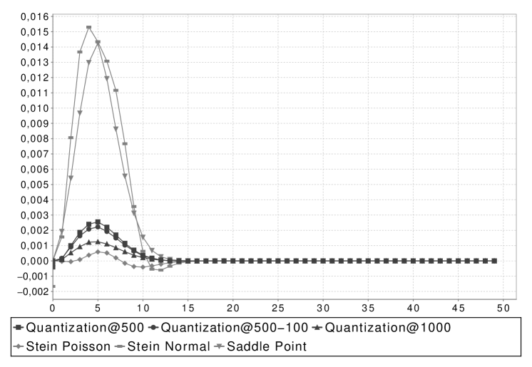
Figure 3: Absolute Errors for the call of various strikes ($p_{0}=0.05,\sigma=0.5$).

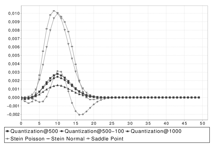
Figure 4: Absolute Errors for the call of various strikes ($p_{0}=0.10,\sigma=0.5$).

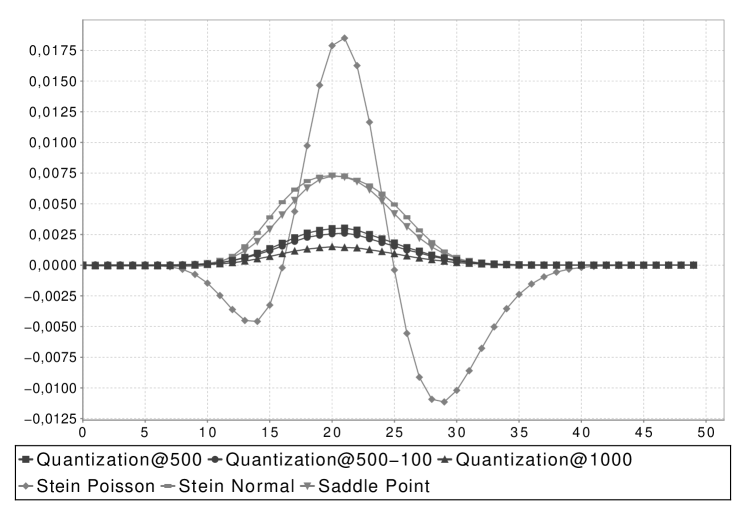
Figure 5: Absolute Errors for the call of various strikes ($p_{0}=0.20,\sigma=0.5$).

Inhomogeneous random walk I.

To discuss a more realistic scenario, we present an inhomogeneous setting with $\alpha_{i}$ uniform distributed on the integers $\{1,2,\cdots,10\}$, so that it is still possible to compute some reference values by means of a recombining binomial tree. The parameters read as follows

• $n=100$,

• $\alpha_{i}\sim\mathcal{U}\{1,2,\cdots,10\}$,

• $p_{i}=p_{0}\,\exp(\sigma\xi_{i}-\sigma^{2}/2),\quad\xi_{i}\sim\mathcal{N}(0,1)$ i.i.d.,

  $p_{0}\in\{0.05,0.2\},\;\sigma=0.5$,

The numerical results are depicted in Figures 6 and 7. Note that we have excluded the Stein-Poisson approach since this setting is already out of the Poisson-limit domain for $p_{0}=0.05$ and consequently yield bad results.

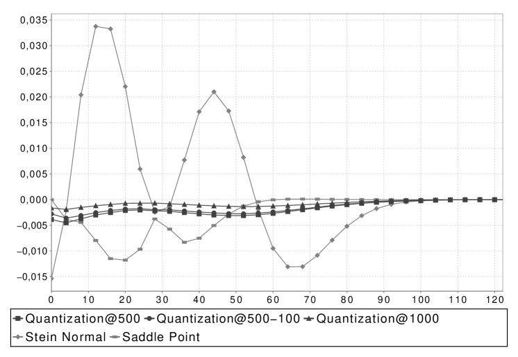
Figure 6: Absolute Errors for the call of various strikes ($p_{0}=0.05,\sigma=0.5$).

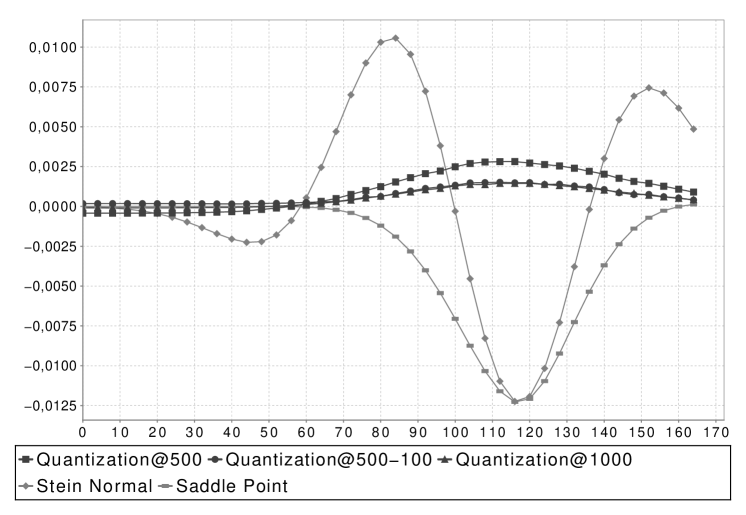
Figure 7: Absolute Errors for the call of various strikes ($p_{0}=0.20,\sigma=0.5$).

Inhomogeneous random walk II.

Finally, we present a non-trivial case, where the $\alpha_{i}$ are non-integer valued any more, i.e. we have chosen them to be $\mathcal{U}([0,1])$ distributed. Since in this setting the recombining property of a binomial tree is destroyed, we cannot compute the exact reference value any more. Therefore, we have chosen a grid of size $N=10000$ to compute a reference value, since such a large grid size yields in all former examples an absolute error less than $10^{-8}$. To be more precise, the parameters has been chosen as follows:

• $n=100$,

• $\alpha_{i}\sim\mathcal{U}([0,1])$,

• $p_{i}=p_{0}\,\exp(\sigma\xi_{i}-\sigma^{2}/2),\quad\xi_{i}\sim\mathcal{N}(0,1)$ i.i.d.,

  $p_{0}\in\{0.05,0.2\},\;\sigma=0.5$.

Since the Figures 8 and 9 are quite similar to those obtained in the first inhomogeneous setting (except a lower resolution), it seems very likely, that the former inhomogeneous setting is a very generic case to illustrate the general performance of the three tested methods.

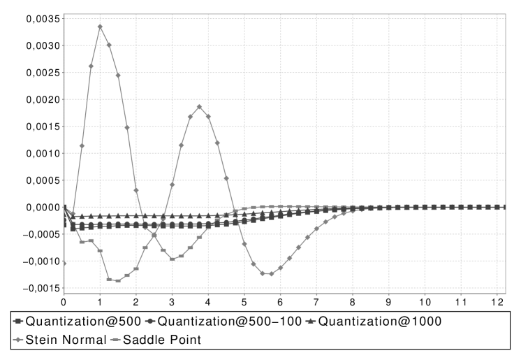
Figure 8: Absolute Errors for the call of various strikes ($p_{0}=0.05,\sigma=0.5$).

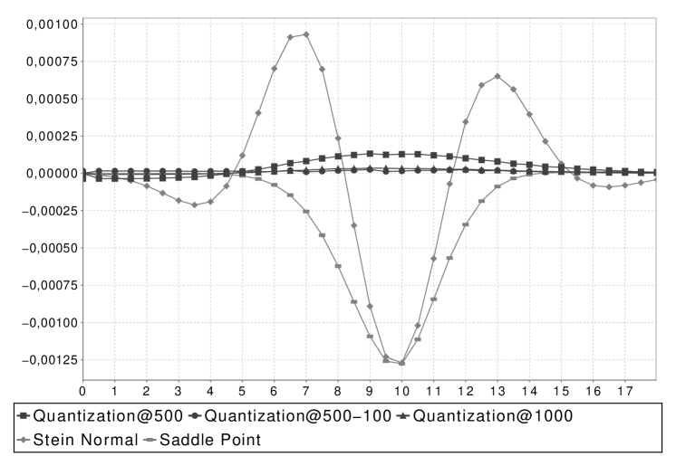
Figure 9: Absolute Errors for the call of various strikes ($p_{0}=0.20,\sigma=0.5$).

In all the above cases the quantization method remains very stable and outperforms even for a grid size of $N=500$ in nearly all cases the other tested methods. Only in the homogeneous setting and for very small probabilities $p_{i}$, it cannot achieve the performance of the Stein-Poisson approximation. However, this excellence of the Stein-Poisson method in that particular setting is mainly caused by the fact, that the target distribution is an integer-valued one, as the Possion approximation is. Hence, these result are nontransferable to the inhomogeneous case.

In the more complex inhomogeneous setting (Figures 6 and 7), we still observe a strong domination of the quantization methods for small and moderate probabilities. Furthermore, in the case $p_{0}=0.2$, we even get an error for the Romberg extrapolation with grid sizes $500$ and $100$, which is close to that of a $1000$-point quantization.

Concerning the computational time for the processing of our Dual Quantization algorithm, this approach is of course not as fast as the Stein’s method, where one only needs to compute the two first moments of $X$ and then evaluates the CDF-function of the standard normal distribution. To apply our scheme, we have to process at each layer $k,0\leq k\leq n$ at full grid $\Gamma_{k}$ similar to recombining tree methods. Nevertheless, the execution of Algorithm 1 implemented in C# on a Intel Xeon CPU@3GHz took for a grid size of $N=500$ only a few milliseconds. Moreover, once the distribution of $\widehat{X}^{n}$ is established, we compute $\mathbb{E}(\widehat{X}^{n}-K)_{+}$ for several strikes $K$ (as needed in practical applications) in nearly no time.

Finally, we want to emphasize, that this approach gives, through the freedom to choose a larger grid size, a control on the acceptable error for the approximation.

4 Approximation of the Greeks

Concerning the computation of sensitivities with respect to the parameters $\alpha_{l}$ and $p_{l},1\leq l\leq n$, we consider $f:\mathbb{R}^{n}_{+}\times(0,1)^{n}\to\mathbb{R},$ defined by

$$(\alpha,p)\mapsto f(\alpha,p):=\mathbb{E}\Bigl{(}\sum_{i=1}^{n}\alpha_{i}Z_{i}-K\Bigr{)}^{+}.$$

We are now interested in the computation of $\frac{\partial f}{\partial p_{l}}$ and $\frac{\partial f}{\partial\alpha_{l}}$.

Some elementary calculations reveal that for every $l\in\{0,\ldots,n\}$

$$\frac{\partial f}{\partial p_{l}}=\mathbb{E}\Bigl{(}\sum_{i\neq l}\alpha_{i}Z_{i}-(K-\alpha_{l})\Bigr{)}^{+}-\mathbb{E}\Bigl{(}\sum_{i\neq l}\alpha_{i}Z_{i}-K\Bigr{)}^{+}$$

and

$$\frac{\partial f}{\partial\alpha_{l}}=p_{l}\cdot\mathbb{P}\Bigl{(}\sum_{i\neq l}\alpha_{i}Z_{i}\geq K-\alpha_{l}\Bigr{)},$$

so that our task consists of approximating the distribution of

$$\partial_{l}X:=\sum_{i\neq l}\alpha_{i}Z_{i}.$$

This can be achieved using a straightfoward adaption of the previous dual quantization tree, where we simply skip the $l$-th layer.

To be more precise, we set

$$\begin{split}\widehat{\partial_{l}X^{0}}&:=0\\ \widehat{\partial_{l}X^{k}}&:=\begin{cases}\mathcal{J}^{\Lambda_{k}}_{\Gamma_{k}}\!(\widehat{X}^{k-1}+\alpha_{k}Z_{k})&k\neq l,\\ \widehat{\partial_{l}X^{k-1}}&k=l.\\ \end{cases}\end{split}$$

Remark.

This scheme can be processed simultaneously for all $l,\;1\leq l\leq n$ without increasing the number of nearest neighbor searches.

Numerical experiments, which are not reproduced here, also confirm the good numerical performance of the dual quantization in this specific setting.

Acknowledgements

We are very thankful to F.X. Vialard from Zeliade Systems for helpful discussions and comments during our work on this topic.

References

• [1] L. Andersen, J. Sidenius, and S. Basu. All your hedges in one basket. Risk magazine, November, 2003.
• [2] N. El Karoui and Y. Jiao. Stein’s method and zero bias transformation for CDO tranche pricing. Finance Stoch., 13(2):151–180, 2009.
• [3] R. Frey, AJ. McNeil, and M. Nyfeler. Copulas and credit models. Risk magazine, October, 2001.
• [4] S. Graf and H. Luschgy. Foundations of Quantization for Probability Distributions. Lecture Notes in Mathematics $n^{0}$1730. Springer, Berlin, 2000.
• [5] J.-P. Laurent and J. Gregory. Basket default swaps, cdo’s and factor copulas. Journal of Risk, 7(4):103–122, 2005.
• [6] D.X. Li. On default correlation: A copula function approach. Journal of Fixed Income, 9(4):43–54, 2000.
• [7] R. Martin, K. Thompson, and C. Browne. Taking to the saddle. Risk magazine, June, 2001.
• [8] G Pagès. Quadratic optimal functional quantization of stochastic processes and numerical applications. In A. Keller, S. Heinrich, and H. Niederreiter, editors, Monte Carlo and Quasi-Monte Carlo Methods 2006, pages 101–142. Springer-Verlag, Berlin, 2008.
• [9] G. Pagès and J. Printems. Optimal quadratic quantization for numerics: the Gaussian case. Monte Carlo Methods and Applications, 9(2):135–166, 2003.
• [10] G. Pagès and J Printems. www.quantize.maths-fi.com. website devoted to quantization, 2005. maths-fi.com.
• [11] G. Pagès and B. Wilbertz. Dual quantization. Work in progress, 2009.