Determination of $B_{K}$ using improved staggered fermions (III) Finite volume effects

Abstract:

We study the finite-volume effects in our calculation of $B_{K}$ using HYP-smeared improved staggered valence fermions. We calculate the predictions of both SU(3) and SU(2) staggered chiral perturbation theory at one-loop order. We compare these to the results of a direct calculation, using MILC coarse lattices with two different volumes: $20^{3}$ and $28^{3}$. From the direct calculation, we find that the finite volume effect is $\approx 2\%$ for the SU(3) analysis and $\approx 0.9\%$ for the SU(2) analysis. We also show how the statistical error depends on the number of measurements made per configuration, and make a first study of autocorrelations.

1 Introduction

This paper is the third in a series of four reports on our calculation of $B_{K}$ using HYP-smeared staggered fermions. In the previous two reports we presented the results of our analysis using, respectively, SU(3) and SU(2) staggered chiral perturbation theory (SChPT) [1, 2]. Here we explain how we estimate the finite-volume error, and discuss issues concerning the statistical error. The calculations use the MILC ensembles (C3) and (C3-2), the parameters of which are given in Table 1.

parameter	value
$\beta$	6.76 ($N_{f}=2+1$ unquenched QCD)
$1/a$	1.588(19) GeV
geometry	$20^{3}\times 64$ (C3) and $28^{3}\times 64$ (C3-2)
configurations	671 ($20^{3}$) and 274 ($28^{3}$)
measurements per conf.	9 ($20^{3}$) and 8 ($28^{3}$)
sea quark (asqtad) masses	$am_{l}=0.01$, $am_{s}=0.05$
valence quark (HYP-smeared) masses	0.005, 0.01, 0.015, …, 0.04, 0.045, 0.05

Table 1: Ensembles used to study finite volume effects.

2 Finite Volume Correction: Theory

Finite volume (FV) effects are predicted by ChPT, and are caused by pseudo-Goldstone bosons (PGBs) in loops propagating from their starting point to a periodic image. Experience indicates that the one-loop calculation is a good guide to the sign and rough magnitude of the FV effect (when compared to numerical results or higher order calculations), although it tends to underestimate the size by factors of two or so. We have calculated the one-loop FV effects using SChPT for both SU(2) and SU(3) formulae. These enter in the standard way through the chiral logarithmic functions:

$$\ell(X) = X\Big{[}\log(X/\mu^{2}_{\text{DR}})+\delta_{1}^{\text{FV}}(X,L)\Big{]}$$ (1)

$$\tilde{\ell}(X) = -\frac{d\ell(X)}{dX}=-\log(X/\mu^{2}_{\text{DR}})-1+\delta_{3}^{\text{FV}}(X,L)$$ (2)

where $X=M^{2}$ is a PGB mass-squared (in physical units), and the finite-volume corrections are given in terms of modified Bessel functions by

$$\delta_{1}^{\text{FV}}(X,L) = \frac{4}{z}\sum_{\vec{n}\neq 0}\frac{K_{1}(|\vec{n}|z)}{|\vec{n}|}$$ (3)

$$\delta_{3}^{\text{FV}}(X,L) = 2\sum_{\vec{n}\neq 0}K_{0}(|\vec{n}|z)\,.$$ (4)

Here $z=ML$, with $L$ the spatial box size in physical units, and $\vec{n}$ is a vector labeling the spatial image positions, taking values $(1,0,0)$, $(0,1,0)$ etc..

When evaluating the image sums we find that keeping up to $\vec{n}^{2}=12$ in $\delta_{1}^{\rm FV}$ and $\vec{n}^{2}=16$ in $\delta_{3}^{\rm FV}$ gives sufficient accuracy. As a side note, for our range of $z$, $2.5\leq z\leq 10$, it is sometimes useful to have an approximate form to speed up the calculation. We find that

$$\delta^{\rm FV}_{1}(z) \approx e^{-z}z^{-3/2}(26.0095+37.8217/z+112.694/z^{2}-59.9524/z^{3})\,,$$ (5)

$$\delta^{\rm FV}_{3}(z) \approx e^{-z}z^{-1/2}(12.8717+10.7318/z+88.9023/z^{2}-20.8847/z^{3})\,.$$ (6)

gives an accuracy of better than 1 part in $10^{3}$ over this range. Note that these are not asymptotic expansions—these forms fail for both small and large $z$.

In our fitting to SChPT forms (as described in the companion reports [1, 2]) we have, so far, used the infinite-volume expressions. Thus it is important to check that FV corrections are small. Using the coefficients from the fit functions, we can calculate the one-loop expectation for the FV corrections for each fit. For the SU(3) fits, the largest contribution to the FV corrections comes from terms induced by discretization and truncation errors. These are not well determined, with the result that different fits differ even in the sign of the predicted FV effect. Thus we can at most use these calculations to estimate the magnitude of the FV effect.

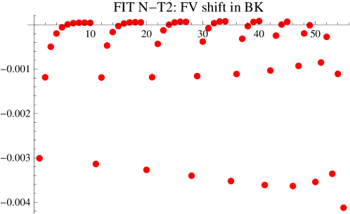
Figure 1: Finite volume shift in $B_{K}$ as predicted by SU(3) SChPT for the $20^{3}\times 64$ coarse MILC lattice, using the “N-T2” fit [3]. The horizontal axis orders the 55 valence “kaons” into groups in which $am_{y}$ is fixed and $am_{x}$ is increased from $0.005$ up to $am_{y}$. The first group (10 leftmost points) have $am_{y}=0.05\approx am_{s}^{\rm phys}$, the next group (9 points) have $am_{y}=0.045$, etc.. The rightmost point has $am_{x}=am_{y}=0.005$. The extrapolation to the physical kaon mass is dominated by the leftmost group. Note that the lowest “row” of points all have $am_{x}=0.005$.

As an example, we show in Fig. 1 the FV correction for the ensemble (C3) using the fit-type which gives rise to the largest FV correction. We see that the effect depends dominantly on the light-quark valence mass $m_{x}$, and much more weakly on the strange valence mass $m_{y}$. It grows rapidly as $m_{x}$ decreases, which is expected given the exponential dependence on $z$. The size of the FV effect is, however, small compared to $B_{K}\approx 0.5$—the relative contribution does not reach 1%. We also note that on the larger, $28^{3}$, lattices, the FV correction is smaller by almost an order of magnitude, and thus negligible compared to other errors.

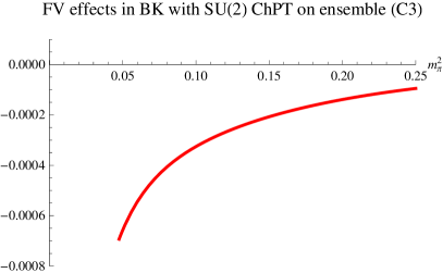
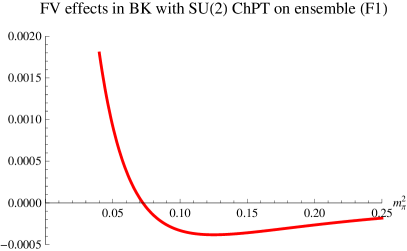
Figure 2: Finite volume correction to $B_{K}$ from SU(2) SChPT as a function of the squared mass of the pion composed of light valence quarks, $M_{\pi}^{2}=X$ in GeV². Left panel: coarse ensemble (C3); right panel: fine ensemble (F1). The lower limit of the curves corresponds to the minimum values of $M_{\pi}^{2}$ in the simulations.

The situation with SU(2) SChPT is shown in Fig. 2, here with results on both coarse and fine lattices. The NLO prediction is more reliable in this case, since the coefficient of the chiral logarithms is well determined by the fits. We see again that the FV effect grows rapidly as $m_{x}\propto M_{\pi}^{2}$ decreases. The size of the effect is, however, very small, significantly smaller than predicted by the SU(3) fit. One peculiar feature is that the sign changes (and magnitude increases) moving from coarse to fine lattices (which are otherwise similar). This is a reflection of the fact that, as one approaches the continuum limit, taste splittings reduce, more pions become lighter, and FV effects increase. In this specific case there are various canceling contributions and it turns out also that the sign flips.

We draw two main conclusions from these results. First, the FV correction to $B_{K}$ is small, comparable to or smaller than the statistical error for our most physical “kaon” (an error which is $\approx 0.6\%$ on the coarse ensemble). Thus we are unlikely to make an error of larger than $\approx 1\%$ by leaving FV corrections out of the fits. Second, we do not know in detail the expected form, or even the sign, of the FV correction. Note that the true FV correction for given valence masses has a definite value, one that SU(2) and SU(3) ChPT should agree upon. The disagreement between the two estimates is thus an indication that the NLO predictions are quantitatively unreliable.

This topic deserves further study. In particular we intend to include one-loop FV corrections in future fits. In the meantime we turn to a more direct method for estimated the FV error.

3 Finite Volume Correction: Direct Measurement

In order to study the finite volume effect numerically, we compare results on the two coarse ensembles whose parameters are listed in Table 1. The lightest valence pion on the smaller lattice has $m_{\pi}L\approx 2.68$. This is below the rule-of-thumb minimum “safe” value of 3-4, but we expect to have more leeway when calculating kaon properties (such as $B_{K}$), since the pion only enters through loops. Indeed, the estimates of the previous section suggest that FV effects remain small. We also note that the same estimates indicate that FV effects are almost negligible on the larger, $28^{3}$, lattices.

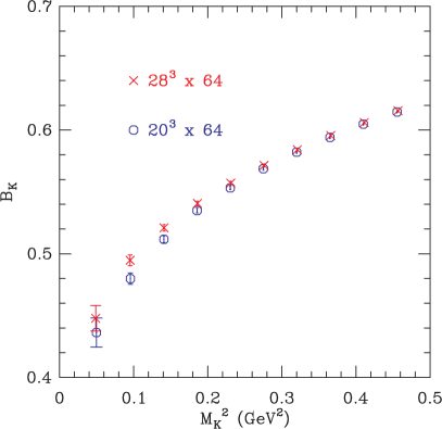
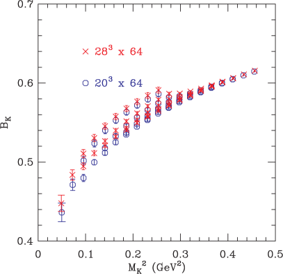
Figure 3: One-loop matched $B_{K}$ vs. $m_{K}^{2}$ for the 10 degenerate combinations (left) and for all 55 degenerate and non-degenerate combinations (right).

We have adjusted the number of measurements per configuration so that the statistical weights of the two ensembles are very similar:

$$\textrm{ratio of stat. weights}=\frac{20^{3}\times 671\times 9}{28^{3}\times 274\times 8}=1.004\,.$$ (7)

In Fig. 3, we show the results for $B_{K}$ on the two lattices, and find that the errors are indeed comparable. The results on the larger lattice lie systematically higher, although for each point the difference is only about 1 $\sigma$. We fit both data-sets using our preferred Bayesian “N-BT7” fit for the SU(3) analysis, and the “4X3Y-NNLO” fit for the SU(2) analysis. The SU(2) “X-fits” are shown in Fig. 4.

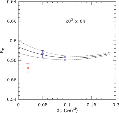
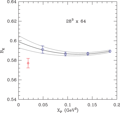
Figure 4: One-loop matched $B_{K}$ vs. $X_{P}$ for the SU(2) analysis on the $20^{3}$ volume (left) and on the $28^{3}$ volume (right). Here $X_{P}$ is the mass-squared of the Goldstone taste “pion” composed of light valence quarks of mass $am_{x}$. See Refs. [1, 2] for more details.

The results of the fits are summarized in Table 2. The difference between $B_{K}$ on the two volumes is $\approx 2\%$ for the SU(3) analysis, which is about twice the statistical error, and thus probably significant. For the SU(2) analysis the finite volume effect is smaller, $\approx 0.9\%$, and, being comparable to the statistical error, less significant. We interpret the difference between SU(3) and SU(2) analyses as being due to greater simplicity of the SU(2) fit form. The size of these effects are not unexpected given the theoretical results of the previous section. We use these differences as estimates of the FV systematic error in the respective fits, as quoted in Refs. [1, 2].

volume	SU(3)	SU(2)
$20^{3}$	0.5599(57)	0.5645(49)
$28^{3}$	0.5730(57)	0.5694(48)

Table 2: Results for $B_{K}$ using SU(3) and SU(2) staggered ChPT. The values quoted are in the NDR scheme at a scale of $\mu=2\;$GeV.

4 Increasing the Statistics and Autocorrelations

It is well know that one can obtain more information from each gauge configuration by using multiple time-positions for the sources. An important issue, however, is the extent to which these measurements are independent. We have tested this by using 9 randomly chosen “starting times” for the wall sources on each configuration in the coarse ensemble (C3), each with a different random seed for the noise in the source. We average the raw data from these 9 sources, and then compute the error using single elimination jackknife. We compare the results so obtained (labeled “x9”) to those obtained using a single measurement/configuration (“x1”) in Fig. 5, displaying only degenerate combinations for clarity. We observe that the errors are reduced by a factor of 3, indicating that the different measurements on each configuration are almost independent.

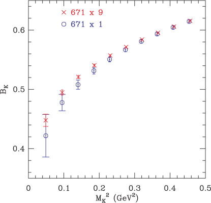
Figure 5: $B_{K}$ vs. $m_{K}^{2}$ on ensemble (C3) for one measurement/conf. and for 9 measurements/conf.

We have also studied autocorrelations between configurations by looking at the dependence of the statistical errors on the bin size (i.e. the number of configurations we bin together) In Fig. 6, we display the result for the error on the 2-point correlator

$$C(t)=\langle A_{4}(t)P(0)\rangle$$ (8)

(where both operators have the Goldstone taste $\xi_{5}$) at $t=10$. For the x1 data, the error in the error bar is too large to determine whether there is an autocorrelation. For the x9 data, however, we do observe about a 20% increase between a bin size of 1 and 3-6. Fortunately this is a small effect. Nevertheless, it is clear that having higher statistics allows us to better understand the autocorrelations, and we intend to increase the statistics on other ensembles as well.

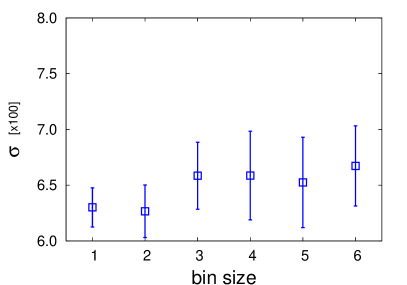
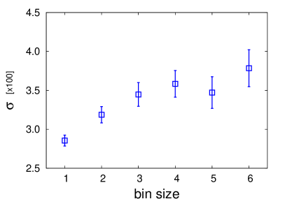
Figure 6: Error in $C(t=10)$ [see text] vs. bin size for the x1 data (left) and the x9 data (right).

5 Acknowledgments

C. Jung is supported by the US DOE under contract DE-AC02-98CH10886. The research of W. Lee is supported by the Creative Research Initiatives Program (3348-20090015) of the NRF grant funded by the Korean government (MEST). The work of S. Sharpe is supported in part by the US DOE grant no. DE-FG02-96ER40956. Computations were carried out in part on facilities of the USQCD Collaboration, which are funded by the Office of Science of the U.S. Department of Energy.

References

- [1] Taegil Bae, et al., PoS (LAT2009) 261.
- [2] Hyung-Jin Kim, et al., PoS (LAT2009) 262.
- [3] Taegil Bae, et al., in preparation.