On the stability of two-chunk file-sharing systems

Abstract

We consider five different peer-to-peer file sharing systems with two chunks, with the aim of finding chunk selection algorithms that have provably stable performance with any input rate and assuming non-altruistic peers who leave the system immediately after downloading the second chunk. We show that many algorithms that first looked promising lead to unstable or oscillating behavior. However, we end up with a system with desirable properties. Most of our rigorous results concern the corresponding deterministic large system limits, but in two simplest cases we provide proofs for the stochastic systems also.

1 Introduction

We consider an open network, with constant rate of incoming ’peers’. A peer is assumed to be able to contact and communicate with any other peer in the system (technically, this can be realised by an overlay network built upon the Internet, where the knowledge of a peer’s IP-address enables communication with it). We assume that one special, persistent peer, the ’seed’, holds a file and wishes to distribute it to all the others. The most effective way of doing this, in particular when the number of peers is very large, is that as soon as a peer receives the file, it becomes a seed itself. The number of copies of the file then grow exponentially. To enhance performance, the file is divided into small chunks that are spread in similar fashion so that parts of the file may start to be multiplied before the original seed has even once uploaded the whole file. This technique was introduced by B. Cohen with his BitTorrent [1] protocol. It became soon the dominant principle of sharing large files (e.g., movies) with peer-to-peer networking.

Moreover, the peers can be ’non-altruistic’ in the sense that they leave the system immediately having downloaded the whole file, without necessarily slowing the system performance. It is remarkable that if there are more than one chunks, it seems that any arrival rate of new peers can still be sustained. However, as we shall see, some additional algorithms are then needed for stable performance. This paper analyses several such algorithms in the simplest relevant case of two chunks. In real systems the number of chunks is large, e.g. of the order $10^{3}$. However, even the case of two chunks, considered here, is highly non-trivial. In fact, it may also be the hardest case as regards stability. For proving stability it is anyway the easiest case, and hopefully the solutions for the two chunk case appear useful in more general models as well.

We work on a fully distributed scenario, relying on randomness: each peer contacts another, uniformly randomly chosen peer, according to a standard Poisson process, and gets to know what chunks the latter possesses. What follows, depends on the particular algorithm. Massoulie and Vojnovic [7] were the first to propose this model and to obtain rigorous mathematical results on it. They allowed an arbitrary number of chunks and analysed the corresponding deterministic large system limit (see Section 2) with the following remarkable result: if each new peer arriving in the system obtains a roughly uniformly random chunk, the system is stable even if all the remaining chunks are downloaded randomly. (In the special case of two chunks, it is noted in [7] that the scheme does not give a unique rest point in the large system limit, but for any larger number of chunks it does.) However, the results of [7] prompt for further research in at least two directions. First, the scheme where the seed gives a uniformly distributed chunk to every new peer makes the seed a potential bottleneck — thus, this algorithm is not as fully distributed as it could be. Second, the stability of the large system limit does not automatically guarantee the stability of the original random system.

We focus on entirely distributed solutions, where also the first chunk must be found randomly from the peer population, and assume ’non-altruistic’ peers. In our first paper [8] we considered the so-called flash-crowd scenario where a large number of peers arrive simultaneously but none afterwards. It was noticed that the first phase of the copying process is asymptotically (with increasing number of peers) equivalent to Pólya’s urn model, which is well known to converge to a random proportion of each chunk in the system. This imbalance leads to the ’rare chunk phenomenon’: one of the chunks is not able to become common and as a result forms a bottleneck of performance (see also [10]). In an open variant of this setup, with continuously incoming peers, this could lead to instability: the number of peers in the system could grow unboundedly, since more and more peers would be searching for the one rare chunk. (BitTorrent counteracts to the rare chunk phenomenon by its ’Rarest First’ principle, and our last two algorithms can be seen as distributed ways to implement this principle using very coarse rarity estimates.) The central question of this paper is: is it possible to avoid the severely imbalanced chunk distribution, implying instability, without using centralized coordination of downloads?

One source of ideas for this is provided by the wide literature on urn models (originally often related to physics; for a recent review, see [9]). For example, Ehrenfests’ urn model gives an almost ideal balance in a closed system. Still more relevant is the so-called Friedman urn, with an analogous result for an open system, with a flow of incoming particles. We showed in [8] that if an empty node first contacts a node having chunk $0$ ($1$) but then downloads the opposite chunk $1$ ($0$) first (neglecting for a while the question how a peer with that chunk could be found), the distribution of chunks converges almost surely to $\frac{1}{2}-\frac{1}{2}$ as the number of peers goes to infinity.

In this paper, we analyse five two-chunk models: (i) the Plain Random Contact system, which is found to be very unstable; (ii) the Deterministic First Chunk system, proposed in [8], but found unstable in the present scenario; (iii) the ideal Friedman system (non-implementable in a distributed way in our scenario), which is proven to be stable; and two distributed algorithms that try to approximate the Friedman system: (iv) the Delayed Friedman system, which may be stable but oscillates heavily, and, finally, (v) the Enforced Friedman system which seems to provide the desired performance.

The paper is structured as follows: general definitions and some preliminaries are given in Section 2, and the five models are studied in Section 3, each in its own subsection. Some concluding remarks are made in Section 4.

2 Definitions and preliminaries

We study time-homogeneous continuous time Markov processes $S=(S_{t})_{t\geq 0}$ with state space $\mathbb{N}^{d}$, where $d$ is 2,3 or 4, depending on the particular model. Denoting the $i$th unit vector by $e_{i}$, $i=1,\ldots,d$, the transitions are always of one of the three forms

$$s\to s+e_{i},\quad s\to s-e_{i},\quad s\to s+e_{i}-e_{j}.$$

Denote the transition intensity from state $\bm{m}$ to state $\bm{n}$ by $q(\bm{m},\bm{n})$. The process $S$ is thought as a model of a queueing network, where the state component $i$ presents the number of customers in network node $i$, $i=1,\ldots,d$.

The Markov process $S$ is called stable, if it is irreducible and positively recurrent. This is equivalent to the existence of a unique stationary probability measure. Assuming irreducibility and finiteness of transition graph neighborhoods, stability is equivalent to the existence of a finite set of states $C\subset\mathbb{N}^{d}$ such that with any starting point $S_{0}$, the process reaches $C$ in a time with finite expectation.

Let $F:(0,\infty)^{d}\to\mathbb{R}^{d}$ be a Lipschitz continuous function so that the autonomous ordinary differential equation

$$\dot{s}=F(s)$$ (1)

has a solution $s(t)$, $t\in[0,T)$, $T\in(0,\infty]$, for every starting point $s(0)\in(0,\infty)^{d}$. We say that the dynamical system (1) is the large system limit of the Markov process $S$, if

$$F_{i}(x)=\lim_{N\to\infty}\left(q(\lfloor Nx\rfloor,\lfloor Nx\rfloor+e_{i})+\frac{1}{N}\sum_{v\not\in\left\{{e_{1},\ldots,e_{d}}\right\}}v_{i}q(\lfloor Nx\rfloor,\lfloor Nx\rfloor+v)\right),\quad i=1,\ldots,d,$$

where $\lfloor y\rfloor$ denotes the largest integer less than or equal to $y$ and is defined componentwise for vectors, and $v=(v_{1},\ldots,v_{d})$ runs over the different possible transition vectors. The idea is to scale the arrival rates to the system (transitions $v=e_{i}$) as well as the states by $N$, divide by $N$ and take the limit. Thus, we assume the internal transition and exit rates to be linear in $N$ as functions of the state. Conditions of limit theorems showing the convergence of the Markov process towards a deterministic limit system in such scaling have been established by Kurtz [5]. This type of results, however, tell nothing about the stability of a stochastic system with finite $N$, and therefore we don’t review them closer here.

The dynamical system (1) is called locally asymptotically stable around an equilibrium state $s^{*}$ (that is, a state with $F(s^{*})=0$), if there exists an open set $U$ containing $s^{*}$ such that $\lim_{t\to\infty}s(t)=s^{*}$ for any initial state $s(0)\in U$. The system is called globally asymptotically stable, if it has a unique equilibrium state $s^{*}$, such that $\lim_{t\to\infty}s(t)=s^{*}$ for any initial state $s(0)\in(0,\infty)^{d}$. Finally, we call the system (1) (globally) stable, if there is a compact set $K\subset(0,\infty)^{d}$ such that for any initial state $s(0)\in(0,\infty)^{d}$ the system reaches $K$ and eventually stays in $K$.

The stability of a large system limit is not known to be sufficient nor necessary for the stability of the original Markov process. We are not aware of any rigorous results concerning this question, but the following remarks illuminate the difficulties in relating the two notions. First, assume that the large system limit exists and is globally asymptotically stable. When $d\geq 3$, the trajectories can however be very complicated and the convergence toward equilibrium very slow. A stochastic system, how well ever fitted to the continuous state space, evolves in jumps and does not follow any trajectory — only its local drift is in the best case close to the derivative of a trajectory passing the same point. Thus, it is hard to imagine how the stability of the stochastic system could be deduced without more specific assumptions. Second, a dynamic system can escape to infinity along a single trajectory (say, along the diagonal) while all other trajectories end to a compact set. In such a case, the stochastic systems with all $N$ could however be stable, since randomness forces them to deviate from the transient trajectory.

However, these circumstances often coincide, and, as we shall see here also, proving the stability of the dynamical system is usually much easier than proving the stability of the Markov process. Therefore it is interesting to consider the large system limits together with the original random systems.

All the systems studied in this paper possess differentiable large system limits, and the existence of a unique solution from any starting point is thus always granted. They are, however, non-linear, and proving their stability seems to be very hard in some cases. There are no black-box tools applicable in general.

The following elementary lemma is sometimes useful when considering the asymptotic behaviour of a dynamical system. For completeness, a proof is given in the Appendix.

Lemma 2.1

Let $a$ and $b$ be Lipschitz continuous functions $[0,\infty)\to(0,\infty)$. The unique solution $u$ of the differential equation

$$\dot{u}_{t}=b_{t}-a_{t}u_{t},\quad t\geq 0,$$

with initial condition $u_{0}\geq 0$ is positive for every $t>0$ and satisfies

$$\frac{\liminf_{t\to\infty}b_{t}}{\limsup_{t\to\infty}a_{t}}\leq\liminf_{t\to\infty}u_{t}\leq\limsup_{t\to\infty}u_{t}\leq\frac{\limsup_{t\to\infty}b_{t}}{\liminf_{t\to\infty}a_{t}}$$

whenever the fractions are well-defined.

3 Models and results

3.1 Plain Random Contact system

Our first and simplest model is defined in Figure 1. The number of non-seed peers with chunk 0 (1) is denoted by $X$ ($Y$). Peers arrive according to a Poisson process with parameter $\lambda$, make a random contact, download whatever chunk the contacted peer has (if the seed was contacted, the downloaded chunk is chosen randomly), then make repeated random contacts at Poisson rate 1 until the remaining chunk is found, and leave the system. The system relies entirely on randomness, with fatal consequences.

Figure 1: Plain Random Contact system

The large system limit of the Plain Random Contact system is the dynamical system defined by the non-linear ordinary differential equations

$$\dot{x}=\frac{(\lambda-y)x}{x+y}\quad\dot{y}=\frac{(\lambda-x)y}{x+y}$$ (2)

This system limit is easily seen to be unstable even close to its equilibirium $x=y=\lambda$:

Proposition 3.1

In $(0,\infty)^{2}$, the system (2) has a single equilibrium $(x^{*},y^{*})=(\lambda,\lambda)$. The system is not stable in any environment of $(x^{*},y^{*})$. Starting with $x_{0}>\lambda>y_{0}$ we have $x_{t}\to\infty$ and $y_{t}\to 0$, and vice versa.

Proof  This is immediate from the equations (2). $\square$

As long as both $x$ and $y$ are large and roughly of the same size, the system empties rapidly. However, it is rather straightforward to prove that the stochastic system is unstable when $\lambda$ is larger than one.

Remark: In this paper, we are not interested in the possible stability of the system when the input rate $\lambda$ is sufficiently low. In all our models, $\lambda$ appears in the large scale limits as a pure scaling parameter that can be as well chosen to be one. The stability of the stochastic system may, however, depend on $\lambda$. Susitaival and Aalto [12] study by simulations several two-chunk systems also from the point of view of stability regions in terms of $\lambda$.

Proposition 3.2

With $\lambda>1$, the (stochastic) Plain Random Contact system is unstable. More exactly, almost surely either $X$ or $Y$ escapes to infinity whereas the other obtains ultimately only the values 0 and 1.

Proof  We couple $(X,Y)$ with a process $(\tilde{X},\tilde{Y})$ such that

1. $\mathbb{P}\left(\forall t\geq 0\ X_{t}\geq\tilde{X}_{t},\,Y_{t}\leq\tilde{Y}_{t}\right)>0$,

2. $\mathbb{P}\left(\lim_{t\to\infty}\tilde{X}_{t}=\infty\right)=1$, and

3. $\mathbb{P}\left(\tilde{Y}_{t}\in\left\{{0,1}\right\}\mbox{ ultimately}\right)=1$.

Assume that $\lambda>1$ and choose a number $a\in(0,\lambda-1)$. Let $\tilde{X}$ and $\tilde{Y}$ be mutually dependent, inhomogeneous birth and death processes with up-jump and down-jump intensities defined as follows, respectively:

$$\alpha^{\tilde{Y}}_{t}=\frac{3\lambda}{2a(t\vee 1)},\quad\beta^{\tilde{Y}}_{t}=\tilde{Y}_{t};\quad\quad\alpha^{\tilde{X}}_{t}=a+1,\quad\beta^{\tilde{X}}_{t}=\ \tilde{Y}_{t}+1.$$

We have

$$\mathbb{P}\left(\tilde{Y}_{t}\geq 1\right)\leq\mathbb{E}\left\{{\tilde{Y}_{t}}\right\}=\int_{0}^{t}\alpha^{\tilde{Y}}_{s}e^{-(t-s)}{\,\mathrm{d}}{s}.$$

Dividing the integration interval into sub-intervals $(0,1]$, $(1,t-2\log t]$ and $(t-2\log t,t]$ we obtain the upper bound

$$\mathbb{P}\left(\tilde{Y}_{t}\geq 1\right)\leq\frac{3\lambda}{2a}\left(e^{-t}+\frac{1}{t^{2}}+\frac{1}{t-2\log t}\right)\sim\frac{3\lambda}{2at}.$$ (3)

Let $N$ denote the counting process of the transitions of $\tilde{Y}$ from 1 to 2. Inequality (3) yields that there are a.s. only finitely many such transitions. Indeed,

$$\mathbb{E}\left\{{N_{\infty}}\right\}=\mathbb{E}\left\{{\int_{0}^{\infty}\alpha^{\tilde{Y}}_{t}1_{\{\tilde{Y}_{t}=1\}}{\,\mathrm{d}}{t}}\right\}\leq\int_{0}^{\infty}\alpha^{\tilde{Y}}_{t}\mathbb{P}\left(\tilde{Y}_{t}\geq 1\right){\,\mathrm{d}}{t}<\infty,$$

since the rightmost integrand is $O(t^{-2})$. Thus, $\tilde{Y}$ has the property (iii). Since

$$\lim_{t\to\infty}\frac{1}{t}\int_{0}^{t}\tilde{Y}_{s}{\,\mathrm{d}}{s}=0<a,$$

we also obtain (ii).

Now, choose $M\in\mathbb{N}$ so large that

$$\frac{\lambda}{\displaystyle 1+\frac{2}{M}}>a+1,$$

set $X_{0}=\tilde{X}_{0}\geq M$, $Y_{0}=\tilde{Y}_{0}=0$ and define

$$\tau=\inf\left\{{t}:\>{\tilde{X}_{t}<at\mbox{ or }\tilde{Y}_{t}>1}\right\}.$$

Then obviously $\mathbb{P}\left(\tau=\infty\right)>0$, and on $\left\{{\tau=\infty}\right\}$ we can couple $(X,Y)$ with $(\tilde{X},\tilde{Y})$ in the desired way thanks to domination relations between the respective intensities. Hence, there exists a positive number $p$ such that

$$\mathbb{P}\left[\left.\lim_{t\to\infty}X_{t}=\infty,\ Y_{t}\in\left\{{0,1}\right\}\mbox{ ultimately}\,\right|X_{0}=x_{0},Y_{0}=0\right]>p>0$$ (4)

when $x_{0}\geq M$. By symmetry, the corresponding relation holds if $X$ and $Y$ are interchanged.

Next, let $R>(3/2)\lambda$ and note that

$$\mathbb{P}\left((X_{t},Y_{t})\in[R\vee M,\infty)\times[R\vee M,\infty)\mbox{ ultimately}\right)=0.$$

Indeed, when $X_{t}\wedge Y_{t}\geq R$, the total output rate of the system is larger than the total input rate $\lambda$:

$$\frac{2(X_{t}\wedge Y_{t})}{\displaystyle 1+\frac{X_{t}\wedge Y_{t}+1}{X_{t}\vee Y_{t}}}>\frac{2}{3}R>\lambda.$$

Thus, $\left\{{X_{t}\wedge Y_{t}\leq R\vee M}\right\}$ is a recurrent event. By inspecting the intensities depicted in Figure 1 it is easy to see that the probability of moving from a state with $X\wedge Y\leq R\vee M$ to a state with $X\wedge Y=0$ before a change in $X\vee Y$ is bounded from below by a positive constant not depending on the value of $X\vee Y$. It follows that

$$\left\{{X_{t}\vee Y_{t}\geq R\vee M,\ X_{t}\wedge Y_{t}=0}\right\}$$

is a recurrent event as well. Now, (4) yields the proposition. $\square$

3.2 Deterministic First Chunk system

Our first attempt to overcome the spontaneous imbalance tendency of the Plain Random Contact system was the Deterministic Last Chunk mechanism introduced in [8], where each peer decides in advance (randomly) which chunk it will download as the last one. The idea was to prevent peers from downloading systematically the rarest chunk as the last one before leaving the system. In the two-chunk case, defined by Figure 2, it might be more natural to speak about the Deterministic First Chunk system. The number of empty peers determined to download chunk 0 (1) first is denoted by $A$ ($B$), while $X$ and $Y$ have their previous meaning.

Figure 2: Deterministic First Chunk system

Although this balancing rule worked promisingly well in our flash-crowd setup with many chunks, the two-chunk system is probably unstable — at least its large system limit

$$\dot{a}=\frac{\lambda}{2}-\frac{ax}{x+y} \dot{b}=\frac{\lambda}{2}-\frac{by}{x+y}$$ (5)

$$\dot{x}=\frac{(a-y)x}{x+y} \dot{y}=\frac{(b-x)y}{x+y}$$

is unstable.

Proposition 3.3

The system (5) has no unique equilibrium — its equilibria form the unbounded curve

$$(a(\theta),b(\theta),x(\theta),y(\theta))=(\theta,\frac{\lambda\theta}{2\theta-\lambda},\frac{\lambda\theta}{2\theta-\lambda},\theta),\quad\theta\in(\frac{\lambda}{2},\infty).$$

Moreover, it has an open set of trajectories where two components (either $x$ and $b$ or $y$ and $a$) grow to infinity while the other two remain bounded.

Proof  Choose the initial values so that

$$x(0)>b(0)>\lambda,\quad y(0)<\frac{1}{2}\lambda,\quad a(0)>\frac{(x(0)+y(0))\lambda}{2x(0)}.$$

Then the same relations hold for the whole paths, as seen, with help of Lemma 2.1, by writing

$$\dot{a} = \frac{x}{x+y}\left(\frac{(x+y)\lambda}{2x}-a\right),$$

$$\dot{b} = \frac{y}{x+y}\left(\frac{\lambda}{2}+\frac{\lambda}{2y}\cdot x-b\right),$$

$$\dot{x}-\dot{b} = \frac{y}{x+y}\left(\frac{x}{y}\left(a-\frac{(x+y)\lambda}{2x}\right)-(x-b)\right).$$

Moreover, $x$ and $b$ grow toward infinity, $y$ decreases and $a$ approaches the value $\lambda/2$. $\square$

We don’t have a proof for the stochastic case, but on the basis of similarity in behavior to the Plain Random Contact system (and supported by some simulations), we conjecture that this system be unstable as well:

Conjecture 3.4

With $\lambda$ large enough, the (stochastic) Deterministic First Chunk system is unstable — a.s., either $X$ or $Y$ escapes to infinity, together with $B$ or $A$, respectively.

However, we don’t fix a conjecture about a Deterministic Last Chunk system with three or more chunks.

3.3 Friedman system

Consider an urn containing balls with two colors. The simplest version of Friedman’s urn [4] works so that one repeatedly picks a random ball from the urn and returns it together with a ball of the opposite color. The proportions of the two colors approach $\frac{1}{2}-\frac{1}{2}$ [3].

We now modify the Plain Random Contact system by assuming (without bothering how this might be realised) that arriving peers make a random contact and then enter the system with a copy of the chunk that the contacted peer did not have (in the case that the seed was contacted, the downloaded chunk is chosen randomly); we call this ’complementary’ random input ’Friedman input’. This system is defined by Figure 3.

Figure 3: Friedman system

The corresponding large system limit is

$$\dot{x}=\frac{(\lambda-x)y}{x+y}\quad\dot{y}=\frac{(\lambda-y)x}{x+y}$$ (6)

Proposition 3.5

The system (6) has a single equilibrium $(x^{*},y^{*})=(\lambda,\lambda)$ which is globally stable.

Proof  The equations tell immediately that with any initial state in $(0,\infty)^{2}$, both $x$ and $y$ converge monotonically to $(\lambda,\lambda)$. $\square$

Moreover, we note that $(x-\lambda)^{2}+(y-\lambda)^{2}$ is monotonically decreasing:

$$\frac{{\,\mathrm{d}}}{{\,\mathrm{d}}{t}}((x-\lambda)^{2}+(y-\lambda)^{2})=-\frac{2}{x+y}\left((x-\lambda)^{2}y+(y-\lambda)^{2}x\right)<0.$$

This observation of a simple Lyapunov function can also be used for proving the stability of the stochastic Friedman system:

Proposition 3.6

The Friedman system defined in Figure 3 is stable for any input rate $\lambda$.

Proof  Denote by $N^{x+}$ and $N^{x-}$ the counting processes of the up- and down-jumps of the process $X$, respectively, so that $X_{t}=X_{0}+\int_{0}^{t}({\,\mathrm{d}}{N^{x+}_{s}}-{\,\mathrm{d}}{N^{x-}_{s}})$. We can then write

$$X^{2}_{t}-X^{2}_{0} = \int_{0}^{t}((X_{s-}+1)^{2}-X_{s-}^{2}){\,\mathrm{d}}{N^{x+}_{s}}-\int_{0}^{t}((X_{s-}-1)^{2}-X_{s-}^{2}){\,\mathrm{d}}{N^{x-}_{s}}$$

$$= \int_{0}^{t}(2X_{s-}+1){\,\mathrm{d}}{N^{x+}_{s}}-\int_{0}^{t}(2X_{s-}-1){\,\mathrm{d}}{N^{x-}_{s}}.$$

(Note that $N^{x-}$ does not jump when $X_{s-}=0$.) The compensators of $N^{x+}$ and $N^{x-}$ are, respectively,

$$A^{x+}_{t}=\int_{0}^{t}\frac{\lambda(Y_{s}+\frac{1}{2})}{X_{s}+Y_{s}+1}{\,\mathrm{d}}{t},\quad A^{x-}_{t}=\int_{0}^{t}\frac{X_{s}(Y_{s}+1)}{X_{s}+Y_{s}+1}{\,\mathrm{d}}{t}.$$

Using similar notation for the process $Y$, we see that the process $X^{2}_{t}+Y^{2}_{t}$ is compensated to a martingale by subtracting from it the process $A_{t}=\int_{0}^{t}a_{s}{\,\mathrm{d}}{t}$, where

$$a=\left(4\lambda(X+\frac{1}{2})(Y+\frac{1}{2})-2X(X-\frac{1}{2})(Y+1)-2(X+1)(Y-\frac{1}{2})Y\right)/(X+Y+1).$$

Denoting $m=X\wedge Y$, $M=X\vee Y$, we have the estimate

$$a = \frac{1}{M+m+1}\left(4\lambda(M+\frac{1}{2})(m+\frac{1}{2})-2M(M-\frac{1}{2})(m+1)-2(M+1)m(m-\frac{1}{2})\right)$$

$$\leq \frac{2M(m+1)}{M+m+1}\left(2\lambda(1+\frac{1}{2M})-M+\frac{1}{2}\right)$$

$$\leq \frac{1}{2}(3\lambda+\frac{1}{2}-M)$$

$$\leq -\frac{1}{4}$$

on the set $\left\{{M>3\lambda+1}\right\}$. Denote $\tau=\inf\left\{{t}:\>{M_{t}\leq 3\lambda+1}\right\}$. Assume now that $M_{0}=X_{0}\vee Y_{0}>3\lambda+1$. Then, the process $B_{t}=X^{2}_{t\wedge\tau}+Y^{2}_{t\wedge\tau}$ is a non-negative supermartingale and thus converges to an integrable limit satisfying $\mathbb{E}\left\{{B_{\infty}}\right\}\leq\mathbb{E}\left\{{B_{0}}\right\}$, and $B_{t}-A_{t\wedge\tau}$ is a martingale (for integrability, note that $B_{t}$ is dominated by $(X_{0}+Y_{0}+N^{x+}_{t}+N^{y+}_{t})^{2}$, where $N^{x+}_{t}+N^{y+}$ is a Poisson process). Since $A_{t\wedge\tau}$ is non-increasing, we have

$$B_{0}\geq B_{0}-\lim_{t\to\infty}\mathbb{E}\left\{{B_{t}}\right\}=-\lim_{t\to\infty}\mathbb{E}\left\{{A_{t\wedge\tau}}\right\}\geq\mathbb{E}\left\{{\int_{0}^{\tau}\frac{1}{4}{\,\mathrm{d}}{t}}\right\}=\frac{1}{4}\mathbb{E}\left\{{\tau}\right\}.$$

Thus, the finite set $\left\{{(x,y)\in\mathbb{N}^{2}}:\>{x\vee y\leq 3\lambda+1}\right\}$ is reached from any fixed initial state outside of it in a time having finite expectation. $\square$

3.4 Delayed Friedman system

Our first distributed implementation of the idea of the Friedman system (see [11]) was the system defined by Figure 4. An arriving peer first makes a random contact and then decides to download first the chunk that the contacted peer does not have (in the case that the seed was contacted, the peer decides randomly). As with the Deterministic First Chunk system, the number of empty peers determined to download chunk 0 (1) first is denoted by $A$ ($B$), while $X$ and $Y$ have the same meaning as before. We call this the Delayed Friedman system, because the subsystem $(X,Y)$ obtains Friedman input with stochastic delay.

Figure 4: Delayed Friedman system.

The corresponding large system limit is the dynamical system

$$\dot{a}=\frac{\lambda y-ax}{x+y} \dot{b}=\frac{\lambda x-by}{x+y}$$ (7)

$$\dot{x}=\frac{(a-y)x}{x+y} \dot{y}=\frac{(b-x)y}{x+y}.$$

This system is difficult to analyse, because it oscillates heavily around its unique equilibrium $(a^{*},b^{*},x^{*},y^{*})=(\lambda,\lambda,\lambda,\lambda)$. The ’logic’ of the oscillating system evolution from an imbalanced state, depicted in Figure 5, is the following:

• there is hardly any input to nor output from $y$

• the ’Friedman rule’ directs input to $a$, which accumulates almost all of it, since $x$ is negligible

• when enough mass has accumulated to $a$, the balance starts to improve

• once $x$ has become macroscopic, $a$ and $y$ empty rapidly

• $b$ has not had time to grow, so we get a situation close to the mirror image of the original.

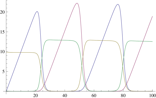
Figure 5: A trajectory of the large system limit (7) of the Delayed Friedman system with initial values $a=b=0$, $x=0.1$, $y=9.9$. Colors: $a$: blue, $b$: red, $x$: green, $y$: brown.

Numerical experiments like that shown in Figure 6 (left) hint to global stability, but we have not found an explicit Lyapunov function or other means to prove this. As regards local behavior near equilibrium, the linearised system at equilibrium is essentially a two-dimensional harmonic oscillator — the two remaining dimensions correspond to negative eigenvalues. If we continue the numerical computation of a trajectory of (7), we see slow convergence toward equilibrium (Figure 6, right; by the way, it is interesting to observe that $x+y$ seems to never descend below 2). Indeed, the system (7) turns out to be locally asymptotically stable, and this can be shown in a non-elementary but basically straightforward way through a center manifold analysis (see [2, 6]).

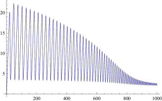
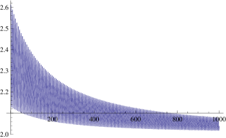
Figure 6: The behaviour of $x+y$, initial state as in Figure 5. Left: $t\in[0,1000]$. Right: $t\in[1000,2000]$.

Proposition 3.7

The system defined by (7) is locally asymptotically stable. If the starting point $(a_{0},b_{0},x_{0},y_{0})$ is close enough to the equilibrium $(\lambda,\lambda,\lambda,\lambda)$, the distance to it decreases proportionally to $1/\sqrt{t}$.

Proof  Since the common denominator of the right hand sides of (7) does not affect the trajectories, and since $\lambda$ is a pure scaling factor, it is sufficient to consider the system

$${\bm{x}}^{\prime}=\begin{bmatrix}x_{4}-x_{1}\,x_{3}\\ x_{3}-x_{2}\,x_{4}\\ (x_{1}-x_{4})\,x_{3}\\ (x_{2}-x_{3})\,x_{4}\end{bmatrix}{\qquad\text{with equilibrium}\qquad}{\bm{p}}=\left[\begin{smallmatrix}1\\ 1\\ 1\\ 1\end{smallmatrix}\right]\ .$$

At ${\bm{p}}$, the linearized system is given by the matrix

$${\bm{A}}=\begin{bmatrix}-1&0&-1&1\\ 0&-1&1&-1\\ 1&0&0&-1\\ 0&1&-1&0\end{bmatrix}\ .$$

This has eigenvalues $\,\lambda_{1,2}=\pm i\,$ and $\,\lambda_{3,4}=-1\,$. The latter has just one linearly independent eigenvector. Let $\,{\bm{v}}_{1}\,$ and $\,{\bm{v}}_{2}\,$ be the real and imaginary parts of an eigenvector corresponding to $\,\lambda_{1}=i\,$ and let $\,{\bm{v}}_{3}\,$ be an eigenvector for $\,\lambda_{3}=-1\,$ and $\,{\bm{v}}_{4}\,$ such that $\,{\bm{A}}\,{\bm{v}}_{4}+{\bm{v}}_{4}={\bm{v}}_{3}\,$. Putting these into matrix $\,{\bm{V}}\,$ we obtain the similarity transformation

$${\bm{V}}^{-1}\,{\bm{A}}\,{\bm{V}}=\begin{bmatrix}0&1&0&0\\ -1&0&0&0\\ 0&0&-1&1\\ 0&0&0&-1\end{bmatrix}{\qquad\text{with}\qquad}{\bm{V}}=\begin{bmatrix}1&1&0&1\\ -1&-1&0&1\\ -1&0&1&0\\ 1&0&1&0\end{bmatrix}\ .$$

Thus, the system has a two-dimensional stable manifold $\,W^{s}\,$ and a two-dimensional center manifold $\,W^{c}\,$. The corresponding columns of $\,{\bm{V}}\,$ are tangents to these at ${\bm{p}}$ (see e.g. [2]), and the manifolds are invariant under the flow of the system. Trajectories close to $\,{\bm{p}}\,$ approach the center manifold like $\,t\,e^{-t}\,$. By the reduction principle (see [6]), in order to study the stability of the system, it suffices to know how it behaves on the local center manifold. For this we will reduce the system to a normal form (see [6]).

Take first a linear change of coordinates:

$${\bm{x}}={\bm{p}}+{\bm{V}}\,\left[\begin{smallmatrix}{\bm{u}}\\ {\bm{v}}\end{smallmatrix}\right]\,,{\qquad\text{where}\qquad}{\bm{u}},{\bm{v}}\in\mathbb{R}^{2}\ .$$

Then the local center manifold can be expressed as

$$W^{c}=\left\{{{\bm{p}}+{\bm{V}}\,\left[\begin{smallmatrix}{\bm{u}}\\ {\bm{h}}({\bm{u}})\end{smallmatrix}\right]}:\>{\|{\bm{u}}\|<d}\right\}\ ,$$

where $\,{\bm{h}}({\bm{u}})\,$ is a two-vector with $\,{\bm{h}}(0,0)=0\,$ and $\,D{\bm{h}}(0,0)=0\,$ (the latter because of tangency).

Write $\,\left[\begin{smallmatrix}{\bm{f}}^{c}\\ {\bm{f}}^{s}\end{smallmatrix}\right]={\bm{V}}^{-1}\,{\bm{f}}\,$. Then the requirement of invariance of $\,W^{c}\,$ amounts to

$${\bm{f}}^{s}({\bm{p}}+{\bm{V}}\,\left[\begin{smallmatrix}{\bm{u}}\\ {\bm{h}}({\bm{u}})\end{smallmatrix}\right])=D{\bm{h}}({\bm{u}})\,{\bm{f}}^{c}({\bm{p}}+{\bm{V}}\,\left[\begin{smallmatrix}{\bm{u}}\\ {\bm{h}}({\bm{u}})\end{smallmatrix}\right])\ .$$

This is the equation for $\,{\bm{h}}\,$. We can recursively solve the coefficients of the Taylor expansion of $\,{\bm{h}}\,$. Note that the constant and linear terms are zero. This way we get:

$${\bm{h}}({\bm{u}})=\tfrac{1}{9}\,\begin{bmatrix}5\,u_{1}^{2}+u_{1}u_{2}-u_{2}^{2}\\ -5\,u_{1}^{2}-14\,u_{1}u_{2}-2\,u_{2}^{2}\end{bmatrix}+O(\|{\bm{u}}\|^{3})$$

and

$${\bm{g}}({\bm{u}}):={\bm{f}}^{c}({\bm{p}}+{\bm{V}}\,\left[\begin{smallmatrix}{\bm{u}}\\ {\bm{h}}({\bm{u}})\end{smallmatrix}\right])=\begin{bmatrix}-u_{2}+(-10\,u_{1}^{3}+8\,u_{1}^{2}u_{2}-2\,u_{1}u_{2}^{2}+u_{2}^{3}\,)/9\,\\ u_{1}\end{bmatrix}+O(\|{\bm{u}}\|^{4})\ .$$

The behaviour of the system on the center manifold is given by equation $\,{\bm{u}}^{\prime}={\bm{g}}({\bm{u}})\,.$ Following [6] we change to complex variables. An eigenvector of the linear part of $\,{\bm{g}}\,$ corresponding to the eigenvalue $\,i\,$ is $\,{\bm{q}}=\left[\begin{smallmatrix}i\\ 1\end{smallmatrix}\right]\,$. Setting $\,{\bm{u}}=z\,{\bm{q}}+\bar{z}\,\bar{\bm{q}}\,$ we get $\,z=(u_{2}-i\,u_{1})/2\,$ and

$$z^{\prime}=i\,z+\tfrac{8+7i}{18}\,z^{3}+\tfrac{32+11i}{18}\,z^{2}\,\bar{z}+\tfrac{32-11i}{18}\,z\,\bar{z}^{2}+\tfrac{-8+7i}{18}\,\bar{z}^{3}+O(\left|z\right|^{4})\ .$$

Taking substitution $\,z=w+\beta_{3}\,w^{3}+\beta_{2}\,w^{2}\,\bar{w}+\beta_{1}\,w\,\bar{w}^{2}+\beta_{0}\,\bar{w}^{3}\,$ we obtain

$$w^{\prime}=i\,w+(\tfrac{8+7i}{18}-2\,\beta_{3})\,w^{3}-\tfrac{32+11i}{18}\,w^{2}\,\bar{w}+(\tfrac{32-11i}{18}+2i\,\beta_{1})\,w\,\bar{w}^{2}+(\tfrac{-8+7i}{18}+4i\,\beta_{0})\,\bar{w}^{3}+O(\left|w\right|^{4})\ .$$

We see that we can kill other third order terms except the $\,w^{2}\,\bar{w}\,$-term. Hence choosing

$$\beta_{0}=\tfrac{7-8i}{72}\,,\ \beta_{1}=\tfrac{11+32i}{36}\,,\ \beta_{2}=0\,,\ \beta_{3}=\tfrac{7-8i}{36}\,,$$

we obtain the equation

$$w^{\prime}=i\,w-\tfrac{32+11i}{18}\,\left|w\right|^{2}\,w+O(\left|w\right|^{4})\ .$$

Now, since

$$\tfrac{d\ }{dt}\left|w\right|^{2}=(i\,w-\tfrac{32+11i}{18}\,\left|w\right|^{2}\,w)\,\bar{w}+w\,(-i\,\bar{w}-\tfrac{32-11i}{18}\,\left|w\right|^{2}\,\bar{w})+O(\left|w\right|^{5})=-\tfrac{32}{9}\left|w\right|^{4}+O(\left|w\right|^{5})\ ,$$

we see that $\,w\to 0\,$ like $\,1/\sqrt{t}\,$. Hence the system is locally asymptotically stable. $\square$

If the third order terms of the equation of $\,w\,$ would not have determined the stability, we should have gone to higher order expansions.

Our simulations showed that also the original stochastic system oscillates strongly, with a roughly constant amplitude depending on $\lambda$, even when it is started from a balanced state. The simulations suggested that the stochastic system might be stable, but we have not found a way to prove or disprove this. From a practical viewpoint, the oscillations indicate that the system is not in good balance, which could be fatal in an application with rapidly changing arrival rates and flash crowd scenarios.

3.5 Enforced Friedman system

The reason of the oscillatory behaviour of the Delayed Friedman system was that when a peer finally succeeds in downloading its first chunk according to the ’Friedman rule’, applied possibly long ago, the choice may already be outdated and thus counterproductive. Our last model avoids this problem by realising choices only immediately or not at all. An empty peer makes three contacts simultaneously (sampling with replacement; the seed shows a random chunk). If two of the chunks of the contacted peers differ from the third one, the latter is downloaded. If all three chunks are similar, nothing is done, but the empty peer stays in a waiting room and repeats the triple contact operation after Exp(1)-distributed waiting time. The number of peers in the waiting room is denoted by $Z$. Note that if the experiment was successful (that is, a 2-1 situation was obtained), the probability of downloading chunk 0 is $(Y+\frac{1}{2})/(X+Y+1)$ — exactly the same as in the Friedman system! Therefore we call this system, defined by Figure 7, the Enforced Friedman system.

Figure 7: Enforced Friedman system.

The large system limit of the Enforced Friedman system is

$$\dot{z} = \lambda-\frac{3xyz}{(x+y)^{2}}$$ (8)

$$\dot{x} = \frac{3xy^{2}z}{(x+y)^{3}}-\frac{xy}{x+y}$$ (9)

$$\dot{y} = \frac{3x^{2}yz}{(x+y)^{3}}-\frac{xy}{x+y}.$$

This is trickier than the plain Friedman system, but nevertheless tractable:

Proposition 3.8

The system (8) has in $(0,\infty)\times(0,\infty)\times(0,\infty)$ a single equilibrium point $(z^{*},x^{*},y^{*})=(\frac{4}{3}\lambda,\lambda,\lambda)$. Locally, the equilibrium is a sink, i.e. all eigenvalues of the limiting linear system are real and negative. This equilibrium is globally asymptotically stable.

Proof  The uniqueness and local character of the equilibrium are found by easy computations. It remains to prove the global stability. Since $\lambda$ is a pure scaling parameter, we can choose $\lambda=1$. Let us change to the variables

$$z,\quad\rho=x+y,\quad\beta=\left(\frac{x-y}{x+y}\right)^{2},$$

which lose the differentiation between $x$ and $y$ in favour of a single imbalance characteristic $\beta$. The new system satisfies the equations

$$\dot{z} = 1-\frac{3}{4}(1-\beta)z$$ (10)

$$\dot{\rho} = \frac{1}{4}(1-\beta)(3z-2\rho)$$ (11)

$$\dot{\beta} = -\beta(1-\beta)\left(\frac{3z}{\rho}-1\right).$$ (12)

Fix arbitrary initial values $z_{0}>0$, $\rho_{0}>0$, $\beta_{0}\in(0,1)$ ($\beta_{0}=0$ gives a simple linear system).

$1^{\mathrm{o}}$. Note first that the system $(z_{t},\rho_{t},\beta_{t})$ cannot escape from the set $(0,\infty)\times(0,\infty)\times[0,1)$ in finite time. Denote $\tau=\inf\left\{{t\geq 0}:\>{\beta_{t}=1}\right\}$. For $t\in[0,\tau)$, $\dot{z}_{t}>0$ whenever $z_{t}<4/3$, and $\dot{\rho}_{t}>0$ whenever $\rho_{t}<(3/2)z_{t}$. Since the system freezes at $\tau$, it follows that $\inf_{t\geq 0}z_{t}\geq\min(z_{0},4/3)$ and $\inf_{t\geq 0}\rho_{t}>0$. Equation (12) then yields that $\beta$ cannot reach 1 at any finite time, so $\tau=\infty$.

$2^{\mathrm{o}}$. A basic observation from the equations (9) is that the absolute value of $x-y$ is non-increasing. In terms of the variables $z,\rho,\beta$ this means that $\beta\rho^{2}$ is non-increasing, and the corresponding equation from which this is seen reads

$$\frac{\mathrm{d}}{\mathrm{d}t}(\beta_{t}\rho^{2}_{t})=-\frac{3}{2}\beta_{t}(1-\beta_{t})z_{t}.$$ (13)

By point $1^{\mathrm{o}}$, we get

$$\lim_{t\to\infty}\int_{t}^{\infty}\beta_{s}(1-\beta_{s})z_{s}{\,\mathrm{d}}{s}=0.$$ (14)

Assume that $\beta_{t}\to 1$. Since $\beta_{t}\rho_{t}^{2}$ is decreasing by (13), $\rho_{t}$ cannot be ultimately increasing, and it approaches some finite limit value. On the other hand, Lemma 2.1, applied to (10), yields with $\beta_{t}\to 1$ that $z_{t}\to\infty$, and (11) makes $\rho_{t}$ ultimately increasing. This contradiction shows that $w:=1-\lim\inf_{t\to\infty}\beta_{t}>0$.

Since we already saw that ultimately $z_{t}\geq 1$, we obtain by (14) and (12) (neglecting the term $3z/\rho$ that for any $\epsilon>0$ there exists a number $t_{0}$ such that

$$\epsilon>\int_{t}^{\infty}\beta_{s}(1-\beta_{s})z_{s}{\,\mathrm{d}}{s}\geq\int_{t}^{T}\dot{\beta}_{s}{\,\mathrm{d}}{s}=\beta_{T}-\beta_{t}$$ (15)

for any $t$ and $T$ such that $T>t>t_{0}$. Choosing $\epsilon=w/2$ we deduce that $\lim\sup_{t\to\infty}\beta_{t}<1$. But then, (14) and (15) imply $\lim_{t\to\infty}\beta_{t}=0$.

$3^{\mathrm{o}}$. Now, Lemma 2.1 yields that $z_{t}$ and $\rho_{t}$ converge to their stable values. $\square$

In simulations, this scheme seems to work in a perfect way, and it is also capable to deal with flash crowds and rapid input rate variations as well (say, when $\lambda$ is large for a while and then suddenly drops). We also have good intuitive grounds to believe that the stochastic Enforced Friedman system be stable: as noted earlier, the output from the waiting room is pure Friedman input to the subsystem $(X,Y)$, just with a randomly varying rate. Since the Friedman system is provably stable with any input rate $\lambda$, the same can be expected from the Enforced Friedman system:

Conjecture 3.9

The (stochastic) Enforced Friedman system is stable with any input rate $\lambda$.

4 Concluding remarks

Although we could so far prove only some of the stability/non-stability properties that seem to hold for our models, some preliminary conclusions can already be drawn. First, we showed that it is possible to create effectively stabilizing ’Friedman input’ using a fully distributed algorithm based on random contacts. Second, one should use a ’waiting room’ concept with memoryless re-trials rather than launch an active hunt for a rare chunk — the rarity may dissolve during the hunt, leading to oscillations. Third, the extra delay caused by the waiting room stage is relatively small in the mean, certainly worth its price. We also believe that the idea of Enforced Friedman input has usable counterparts in many-chunk systems, and we work currently on one promising candidate.

On the other hand, note that our models lack realism as regards the modelling of two aspects of the system: search and downloading. Following [7], the slowness of downloading is modelled by the Exp(1)-distributed inter-contact times, whereas the contacts themselves are assumed to be instant. However, unsuccessful contacts could be repeated much faster than those leading to a chunk download. Assessing the significance of this simplification remains for further work.

Acknowledgement. We thank Balakrishna Prabhu, Rudesindo Nunez Queija, Philippe Robert, Florian Simatos (members of the Euro-FGI SCALP project) and Lasse Leskelä for fruitful discussions and insights.

Appendix A Appendix

Proof  of Lemma 2.1.

Denote $\tau=\inf\left\{{t>0}:\>{u_{t}=0}\right\}$. Since $\dot{u}_{0}=b_{0}>0$ in the case that $u_{0}=0$, we always have $\tau>0$. For $t\in[0,\tau)$ we have

$$\dot{u}_{t}\geq\inf_{s\in[0,\tau)}b_{s}-(\sup_{s\in[0,\tau)}a_{s})u_{t}.$$

It follows that

$$u_{t}\geq\frac{\inf_{s\in[0,\tau)}b_{s}}{\sup_{s\in[0,\tau)}a_{s}}+(u_{0}-\frac{\inf_{s\in[0,\tau)}b_{s}}{\sup_{s\in[0,\tau)}a_{s}})\exp(-(\sup_{s\in[0,\tau)}a_{s})t),\quad t\in[0,\tau).$$

Since the right hand side is positive also for every $t=\tau$, we deduce that $\tau=\infty$.

Assume first that the functions $a$ and $b$ are bounded away from zero and infinity. Let $a_{*},a^{*},b_{*},b^{*}$ be any positive numbers such that

$$a_{*}<\liminf_{t\to\infty}a_{t}\leq\limsup_{t\to\infty}a_{t}<a^{*},\quad b_{*}<\liminf_{t\to\infty}b_{t}\leq\limsup_{t\to\infty}b_{t}<b^{*}.$$

Denote

$$\sigma=\inf\left\{{t\geq 0}:\>{\inf_{s\in[t,\infty)}a_{s}\geq a_{*},\ \sup_{s\in[t,\infty)}a_{s}\leq a^{*},\ \inf_{s\in[t,\infty)}b_{s}\geq b_{*},\ \sup_{s\in[t,\infty)}b_{s}\leq b^{*}}\right\}.$$

Since $\sigma$ is finite and

$$\inf_{s\in[\sigma,\infty)}b_{s}-(\sup_{s\in[\sigma,\infty)}a_{s})u_{\sigma+t}\leq\dot{u}_{\sigma+t}\leq\sup_{s\in[\sigma,\infty)}b_{s}-(\inf_{s\in[\sigma,\infty)}a_{s})u_{\sigma+t},\quad t\geq 0,$$

we obtain that

$$\frac{b_{*}}{a^{*}}+(u_{\sigma}-\frac{b_{*}}{a^{*}})e^{-a^{*}t}\leq u_{\sigma+t}\leq\frac{b^{*}}{a_{*}}+(u_{\sigma}-\frac{b^{*}}{a_{*}})e^{-a_{*}t},\quad t\geq 0,$$

which implies

$$\frac{b_{*}}{a^{*}}\leq\liminf_{t\to\infty}u_{t}\leq\limsup_{t\to\infty}u_{t}\leq\frac{b^{*}}{a_{*}}.$$

Since $a_{*},a^{*},b_{*},b^{*}$ were arbitrary, the assertion follows.

Finally, when $a$ and $b$ are not both bounded away from zero and infinity and the fractions in the assertion are well-defined, the non-trivial cases are obtained as above, simply relaxing some conditions in the definition of $\sigma$. $\square$

References

- [1] B. Cohen. BitTorrent specification, 2006. http://www.bittorrent.org.
- [2] S-N. Chow and J. Hale, Methods of bifurcation theory, Springer-Verlag, New York, 1982.
- [3] D. Freedman. Bernard Friedman’s urn. Ann. Math. Statist., 36:956–970, 1965.
- [4] B. Friedman. A simple urn model. Comm. Pure Appl. Math., 2:59–70, 1949.
- [5] T. Kurtz. Approximation of population processes. CBMS-NSF Regional Conference Series in Applied Mathematics, volume 36, 1981.
- [6] Y. A. Kuznetsov, Elements of applied bifurcation theory, Springer-Verlag, New York, 1995.
- [7] L. Massoulie and M. Vojnovic. Coupon Replication Systems. In Proc. ACM SIGMETRICS, Banff, Canada, 2005.
- [8] I. Norros, B. Prabhu, and H. Reittu. Flash crowd in a file sharing system based on random encounters. In Inter-Perf, Pisa, Italy, October 2006. http://www.inter-perf.org.
- [9] R. Pemantle. A survey of random processes with reinforcement. Probability Surveys, 4:1–79, 2007.
- [10] H. Reittu and I. Norros. Toward modeling of a single file broadcasting in a closed network. In Proceedings of IEEE SPASWIN2007, Limassol, Cyprus, 2007.
- [11] H. Reittu and I Norros. Urn models and peer-to-peer file sharing. In Proc. IEEE PHYSCOMNET’08, Berlin, 2008.
- [12] R. Susitaival and S. Aalto. Analyzing the file availability and download time in a p2p file sharing system. In Proceedings of NGI 2007, 2007.