Cavendish-HEP-09/21

DAMTP-2009-71

Gauge-mediated supersymmetry breaking with generalized messenger sector at LHC

^(a)Hidetoshi Kawase, ^(a)Nobuhiro Maekawa, ^(b)Kazuki Sakurai

^aDepartment of Physics, Nagoya University, Nagoya 464-8602, Japan

^bDAMTP, Wilberforce Road, Cambridge, CB3 0WA, UK
Cavendish Laboratory, JJ Thomson Avenue, Cambridge, CB3 0HE, UK

We consider the generalized gauge mediated supersymmetry breaking (GMSB) models with the messenger fields which do not form the complete multiplets of $SU(5)$ GUT symmetry. Such a situation may happen in the anomalous $U(1)$ GUT scenario because the mass spectrum of the superheavy particle does not respect $SU(5)$ GUT symmetry, although the success of the gauge coupling unification can be explained. In this paper, we assume that one pair of the messenger fields gives the dominant contribution, and the LHC signature for the two possible messengers, $X+\bar{X}$ and $Q+\bar{Q}$, are examined. We investigate the possibility to measure the deviation from the usual GUT relation of the gaugino masses which is one of the most important features of these scenarios.

1 Introduction

The minimal supersymmetric (SUSY) standard model (MSSM) is one of the most promising candidates for the model beyond the standard model (SM) [1, 2, 3]. Unfortunately, the MSSM has more than 100 parameters concerning on the SUSY breaking, and the signatures in the large hadron collider (LHC) are strongly dependent on the parameters, especially, the mass spectrum of SUSY particles [4, 6, 7, 8, 9, 10, 11]. Therefore, it is important to study various possibilities for the SUSY breaking parameters and the LHC signatures before the LHC starts to present the data. In this paper, we examine the generalized gauge mediated SUSY breaking (GMSB) scenario [12, 13, 14] in which the messenger fields do not form the complete grand unified theory (GUT) multiplets.

In the usual GMSB scenario [15, 16], the messenger fields are adopted as complete multiplets under $SU(5)$. This is mainly because the messenger fields which do not respect $SU(5)$ generically spoil the success of the gauge coupling unification in the MSSM. However, it has been understood that the GUT with anomalous $U(1)$ gauge symmetry [17, 18, 19] can naturally explain the success of the gauge coupling unification in the MSSM although the superheavy particles do not respect the $SU(5)$ symmetry [20, 21]. Since some of the superheavy particles can play the same role as the messenger fields, it is important to study the generalized GMSB scenario with the messenger fields which do not form the complete multiplets of $SU(5)$.

One of the most interesting facts in this scenario is that the GUT relation for the gaugino masses are spoiled although the anomalous $U(1)$ GUT has the GUT gauge symmetry at the GUT scale. Actually, if we assume that the SUSY is broken by some mechanism and the resulting superpotential has a form

$$W=m_{\Phi}\Phi\bar{\Phi}+\theta^{2}F_{\Phi}\Phi\bar{\Phi},$$ (1.1)

where $\theta^{2}$ is a superspace coordinate, the masses of gauginos and sfermions at the scale $m_{\Phi}$ are generated by one and two loop effects of the messenger fields $\Phi$ and $\bar{\Phi}$ as [15, 16]

$$M_{a}=n_{a}\left(\frac{\alpha_{a}}{4\pi}\right)\frac{F_{\Phi}}{m_{\Phi}}+\mathcal{O}\left(\frac{F_{\Phi}^{3}}{m_{\Phi}^{5}}\right),$$ (1.2)

$$m_{\tilde{f}}^{2}=\mathop{\mathchoice{\textstyle\sum@}{\textstyle\sum@}{\scriptstyle\sum@}{\scriptscriptstyle\sum@}}\limits_{a=1}^{3}n_{a}C_{a}^{\tilde{f}}\left(\frac{\alpha_{a}}{4\pi}\right)^{2}\frac{F_{\Phi}^{2}}{m_{\Phi}^{2}}+\mathcal{O}\left(\frac{F_{\Phi}^{4}}{m_{\Phi}^{6}}\right),$$ (1.3)

respectively. Here $n_{a}$ ($a=1,2,3$) is the Dynkin index whose normalization is chosen to be $n_{a}=1$ for $\bm{5}+\bar{\bm{5}}$ of $SU(5)$, and $C_{a}^{\tilde{f}}$ is the quadratic Casimir invariant of sfermions. $C_{a}^{\tilde{f}}$ are in a normalization where $C_{1}^{\tilde{f}}=3/5\cdot Y^{2}$ for sfermions with hypercharge $Y$, $C_{2}^{\tilde{f}}=3/4$ for $SU(2)_{L}$ doublets and $C_{3}^{\tilde{f}}=4/3$ for $SU(3)_{C}$ triplets. $n_{a}$ for various messenger fields are given in Table 1. The generalized messenger scenario has a lot of possibilities in general [12, 13]. Here, just for simplicity, we assume that one of the messenger fields in Table 1 dominates. Then only two possibilities, $X+\bar{X}$ and $Q+\bar{Q}$, can give the non-vanishing masses to all the gauginos. In this paper, we examine these two possibilities.

	$\quad(SU(3)_{C},SU(2)_{L})_{U(1)_{Y}}$	$\quad n_{1}\quad$	$\quad n_{2}\quad$	$\quad n_{3}\quad$
$\quad Q+\bar{Q}\quad$	$\quad(\bm{3},\bm{2})_{1/6}+(\bar{\bm{3}},\bm{2})_{-1/6}$	$1/5$	$3$	$2$
$U+\bar{U}$	$\quad(\bm{3},\bm{1})_{2/3}+(\bar{\bm{3}},\bm{1})_{-2/3}$	$8/5$	$0$	$1$
$D+\bar{D}$	$\quad(\bm{3},\bm{1})_{-1/3}+(\bar{\bm{3}},\bm{1})_{1/3}$	$2/5$	$0$	$1$
$L+\bar{L}$	$\quad(\bm{1},\bm{2})_{-1/2}+(\bm{1},\bm{2})_{1/2}$	$3/5$	$1$	$0$
$E+\bar{E}$	$\quad(\bm{1},\bm{1})_{-1}+(\bm{1},\bm{1})_{1}$	$6/5$	$0$	$0$
$G$	$\quad(\bm{8},\bm{1})_{0}$	$0$	$0$	$3$
$W$	$\quad(\bm{1},\bm{3})_{0}$	$0$	$2$	$0$
$X+\bar{X}$	$\quad(\bm{3},\bm{2})_{-5/6}+(\bar{\bm{3}},\bm{2})_{5/6}$	$5$	$3$	$2$

Table 1: The Dynkin indices $n_{a}$ $(a=1,2,3)$ for various messenger fields.

2 Overview of the mass spectrum

As discussed in the introduction, the GUT relation for the gaugino masses is generally spoiled in the generalized GMSB scenario. Since $M_{a}\alpha_{a}^{-1}$ is one-loop renormalization group invariant, the gaugino masses satisfy the relation

$$M_{1}:M_{2}:M_{3}\sim n_{1}\alpha_{1}:n_{2}\alpha_{2}:n_{3}\alpha_{3}$$ (2.1)

at any renormalization scale. Therefore, if we consider a model with messengers which respect $SU(5)$ symmetry, the ratio of gaugino masses at weak scale is given as

$$M_{1}(m_{Z}):M_{2}(m_{Z}):M_{3}(m_{Z})\sim 1:2:6.$$ (2.2)

The relation (2.2) is often called the GUT relation of the gaugino masses. However, this relation is spoiled if $n_{1}=n_{2}=n_{3}$ is not satisfied as in the generalized GMSB scenario. In the followings, we examine the spectra of models with $X+\bar{X}$ or $Q+\bar{Q}$ messengers as a specific example of such scenarios. The parameters for the SUSY breaking sector are $\Lambda_{\Phi}\equiv F_{\Phi}/m_{\Phi}$, $m_{\Phi}$, $\tan\beta$ (the ratio of the VEVs of up-type Higgs and the down-type Higgs), and $\mathrm{sgn}\,(\mu)$ (the sign of the SUSY Higgs mass). The masses of gauginos and sfermions, and the scalar trilinear couplings $A$ at the mass scale of the messenger fields are given as

$$M_{a}(m_{\Phi})\simeq n_{a}\left(\frac{\alpha_{a}}{4\pi}\right)\Lambda_{\Phi},\qquad m_{\tilde{f}}^{2}(m_{\Phi})\simeq\mathop{\mathchoice{\textstyle\sum@}{\textstyle\sum@}{\scriptstyle\sum@}{\scriptscriptstyle\sum@}}\limits_{a=1}^{3}n_{a}C_{a}^{\tilde{f}}\left(\frac{\alpha_{a}}{4\pi}\right)^{2}\Lambda_{\Phi}^{2},\qquad A(m_{\Phi})\simeq 0.$$ (2.3)

We use the renormalization group equations (RGEs) to obtain these parameters at the weak scale. For implementing the numerical calculation, we use SOFTSUSY 2.0.18 [22] with appropriate modification according to our purpose. In our calculation, we assume that the contributions from messenger fields other than the selected one are relatively small and can be neglected entirely. To specify the SUSY Higgs mass $\mu$ and the Higgs mixing parameter $b$ we use the relations

$$b=\frac{1}{2}(m_{H_{u}}^{2}+m_{H_{d}}^{2}+2|\mu|^{2})\sin 2\beta$$ (2.4)

and

$$|\mu|^{2}=\frac{m_{H_{d}}^{2}-m_{H_{u}}^{2}\tan^{2}\beta}{\tan^{2}\beta-1}-\frac{m_{Z}^{2}}{2}.$$ (2.5)

where $m_{H_{u}}^{2}$ and $m_{H_{d}}^{2}$ are the SUSY breaking Higgs mass parameters at the weak scale which are calculated by the RGEs with the boundary values given by (2.3) at the scale $m_{\Phi}$.

First, we consider the scenario with $X+\bar{X}$ messenger. In this scenario, the Dynkin indices are given by

$$n_{1}=5,\qquad n_{2}=3,\qquad n_{3}=2$$ (2.6)

as shown in Table 1, so gaugino masses at the weak scale satisfy the relation

$$M_{1}(m_{Z}):M_{2}(m_{Z}):M_{3}(m_{Z})\sim 5:6:12$$ (2.7)

at one-loop order. Since the relation (2.7) is not affected so much by the specific choice of the parameters such as the mass scale of messenger particles, we can use this relation to distinguish this model from others. The relation (2.7) indicates that the hierarchy among the gaugino masses becomes milder than the usual GUT relation. One of the most interesting features is that the mass splitting between the bino and wino is especially small. Therefore, to check this feature is one of the promising ways to test this scenario.

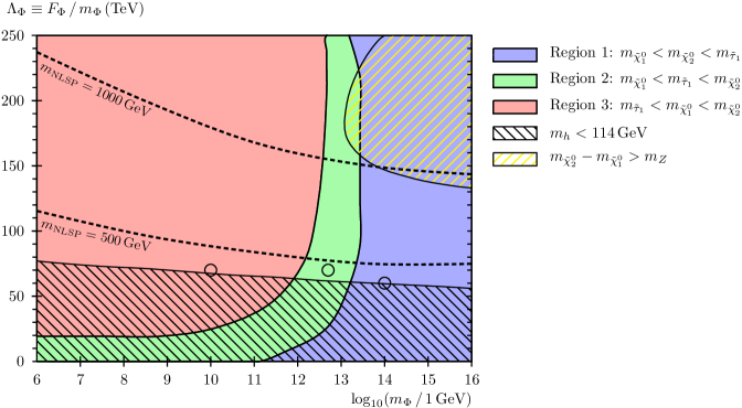
Figure 1: Allowed parameter region for $X+\bar{X}$ messenger scenario. We set $\tan\beta=10$ and $\mathrm{sgn}\,(\mu)=+1$. The circles correspond to the model points selected to analyze the LHC signature.

Figure 1 represents the parameter space in this scenario. Here we set $\tan\beta=10$ and $\mathrm{sgn}\,(\mu)=+1$, and we assume that the lightest SUSY particle (LSP) is the gravitino. The experimental bound for this scenario comes mainly from the LEP2 bound on the lightest Higgs mass $m_{h}>114.4\,\mathrm{GeV}$ [23]. The mass of Higgs is, however, largely dependent on the mass of top quark, so there remains a large uncertainty concerning this bound. We set $m_{t}=175\,\mathrm{GeV}$ for our calculation. As shown in Figure 1, there are three parameter regions, corresponding to

1. $m_{\tilde{\chi}_{1}^{0}}<m_{\tilde{\chi}_{2}^{0}}<m_{\tilde{\tau}_{1}}$

2. $m_{\tilde{\chi}_{1}^{0}}<m_{\tilde{\tau}_{1}}<m_{\tilde{\chi}_{2}^{0}}$

3. $m_{\tilde{\tau}_{1}}<m_{\tilde{\chi}_{1}^{0}}<m_{\tilde{\chi}_{2}^{0}}$.

When the $\Lambda_{\Phi}$ is comparatively small, the higgsinos are relatively heavy compared with the gauginos, and therefore we can roughly identify the lightest neutralino $\tilde{\chi}_{1}^{0}$ with the bino and the second lightest neutralino $\tilde{\chi}_{2}^{0}$ with the wino. Therefore, the bino-like neutralino $\tilde{\chi}_{1}^{0}$ becomes the next to LSP (NLSP) in the regions 1 and 2, and the stau $\tilde{\tau}_{1}$ becomes the NLSP in the region 3.

Figure 2: Allowed parameter region for $Q+\bar{Q}$ messenger scenario. We set $\tan\beta=10$ and $\mathrm{sgn}\,(\mu)=+1$. The circle corresponds to the model point selected to analyze the LHC signature.

Another candidate of messenger fields in our scenario is the fields with quantum number of $Q+\bar{Q}$. In this scenario, the Dynkin indices are given as

$$n_{1}=\frac{1}{5},\qquad n_{2}=3,\qquad n_{3}=2$$ (2.8)

and gaugino masses satisfy the relation

$$M_{1}(m_{Z}):M_{2}(m_{Z}):M_{3}(m_{Z})\sim\frac{1}{5}:6:12$$ (2.9)

at one-loop order. As can be seen from this relation, $Q+\bar{Q}$ messenger scenario gives rather small masses to sparticles which do not have quantum numbers of $SU(2)_{L}$ and $SU(3)_{C}$ compared with the other sparticles. The allowed parameter space is presented in Figure 2. In the whole allowed region, $m_{\tilde{\chi}_{1}^{0}}<m_{\tilde{\tau}_{1}}<m_{\tilde{\chi}_{2}^{0}}$ is satisfied as in the region 2 of $X+\bar{X}$ messenger scenario, and therefore the NLSP is the bino-like neutralino $\tilde{\chi}_{1}^{0}$.

Note that there are almost no bounds for the mass of the lightest neutralino $\tilde{\chi}_{1}^{0}$ if $\tilde{\chi}_{1}^{0}$ is the pure bino and does not decay inside the detector. The GUT relation is essential to obtain the bound $m_{\tilde{\chi}_{1}^{0}}>46\,\mathrm{GeV}$ given by the particle data group [23] and the constraint from the invisible decay of $Z$ is useless because the decay width of $Z\to\tilde{\chi}_{1}^{0}\,\tilde{\chi}_{1}^{0}$ is quite small for the bino-like $\tilde{\chi}_{1}^{0}$ [24]. Therefore the constraint for the mass of right-handed stau $\tilde{\tau}_{1}$, $m_{\tilde{\tau}}>81.9\,\mathrm{GeV}$ is important in this scenario which is shown in Figure 2.

3 LHC signature

In this section, we investigate the LHC signatures of these scenarios. For this purpose, we use ISAJET 7.79 [25] to calculate the decay width of sparticles and HERWIG 6.510 [26, 27] to generate the sparticle production events by Monte-Carlo simulation. And for the detector simulation, we use AcerDET 1.0 [28] as a fast simulation of the search at the LHC. We examine the LHC signatures for $\sqrt{s}=14\,\mathrm{TeV}$ for the whole analysis in this paper.

	$\Lambda_{\text{mess}}$	$m_{\text{mess}}$	$\tan\beta$	$\mathrm{sgn}\,(\mu)$	$n_{1}$	$n_{2}$	$n_{3}$
	(TeV)	(GeV)
Case 1: $m_{\tilde{\chi}_{1}^{0}}<m_{\tilde{\chi}_{2}^{0}}<m_{\tilde{l}_{R}}$	$60$	$1.0\times 10^{14}$	$10$	$+$	$5$	$3$	$2$
Case 2: $m_{\tilde{\chi}_{1}^{0}}<m_{\tilde{l}_{R}}<m_{\tilde{\chi}_{2}^{0}}$	$70$	$5.0\times 10^{12}$	$10$	$+$	$5$	$3$	$2$
Case 3: $m_{\tilde{l}_{R}}<m_{\tilde{\chi}_{1}^{0}}<m_{\tilde{\chi}_{2}^{0}}$	$70$	$1.0\times 10^{10}$	$10$	$+$	$5$	$3$	$2$

Case 1 Case 2 Case 3 $\quad\tilde{g}\quad$ 910 1049 1054 $\tilde{u}_{L}$ 1017 1168 1163 $\tilde{u}_{R}$ 946 1086 1089 $\tilde{d}_{L}$ 1022 1173 1169 $\tilde{d}_{R}$ 905 1047 1063 $\tilde{b}_{1}$ 894 1036 1053 $\tilde{b}_{2}$ 929 1073 1085 $\tilde{t}_{1}$ 704 831 879 $\tilde{t}_{2}$ 957 1097 1107 $\tilde{\nu}_{l}$ 564 621 556 $\tilde{\nu}_{\tau}$ 562 619 555 $\tilde{e}_{L}$ 569 626 561 $\tilde{e}_{R}$ 478 497 403 $\tilde{\tau}_{1}$ 473 492 399 $\tilde{\tau}_{2}$ 568 625 561 $\tilde{\chi}_{1}^{0}$ 395 464 459 $\tilde{\chi}_{2}^{0}$ 439 514 508 $\tilde{\chi}_{3}^{0}$ 530 595 562 $\tilde{\chi}_{4}^{0}$ 571 640 621 $\tilde{\chi}_{1}^{\pm}$ 433 506 496 $\tilde{\chi}_{2}^{\pm}$ 568 636 618 $h^{0}$ 114 115 114 $H^{0}$ 766 852 783 $A^{0}$ 765 851 783 $H^{\pm}$ 770 856 787

Case 1 Case 2 Case 3 $\tilde{u}_{L}\to\tilde{g}\,u$ $.23$ $.23$ $.20$ $\phantom{\tilde{u}_{L}}\to\tilde{\chi}_{1}^{+}\,d$ $.41$ $.39$ $.34$ $\phantom{\tilde{u}_{L}}\to\tilde{\chi}_{2}^{0}\,u$ $.21$ $.21$ $.18$ $\tilde{d}_{L}\to\tilde{g}\,d$ $.25$ $.24$ $.22$ $\phantom{\tilde{d}_{L}}\to\tilde{\chi}_{1}^{-}\,u$ $.41$ $.35$ $.29$ $\phantom{\tilde{d}_{L}}\to\tilde{\chi}_{2}^{0}\,d$ $.21$ $.14$ $.10$ $\tilde{u}_{R}\to\tilde{g}\,u$ $.18$ $.16$ $.14$ $\phantom{\tilde{u}_{R}}\to\tilde{\chi}_{1}^{0}\,u$ $.67$ $.71$ $.63$ $\phantom{\tilde{u}_{R}}\to\tilde{\chi}_{2}^{0}\,u$ $.13$ $.12$ $.22$ $\tilde{d}_{R}\to\tilde{\chi}_{1}^{0}\,d$ $.83$ $.84$ $.69$ $\phantom{\tilde{d}_{R}}\to\tilde{\chi}_{2}^{0}\,d$ $.15$ $.14$ $.24$ $\tilde{g}\to\tilde{t}_{1}\,\bar{t}+\tilde{t}_{1}^{*}\,t$ $.98$ $.98$ $\phantom{\tilde{g}}\to\tilde{\chi}_{2}^{+}\,b\,\bar{t}+\tilde{\chi}_{2}^{-}\,t\,\bar{b}$ $.32$ $\phantom{\tilde{g}}\to\tilde{\chi}_{3,4}^{0}\,t\,\bar{t}$ $.32$ $\tilde{\chi}_{2}^{0}\to\tilde{\chi}_{1}^{0}\,q\,\bar{q}$ $.42$ $\phantom{\tilde{\chi}_{2}^{0}}\to\tilde{\chi}_{1}^{0}\,b\,\bar{b}$ $.12$ $\phantom{\tilde{\chi}_{2}^{0}}\to\tilde{\chi}_{1}^{0}\,l^{+}\,l^{-}$ $.15$ $\phantom{\tilde{\chi}_{2}^{0}}\to\tilde{\chi}_{1}^{0}\,\tau^{+}\,\tau^{-}$ $.10$ $\tilde{\chi}_{2}^{0}\to\tilde{l}^{\pm}_{R}\,l^{\mp}$ $.54$ $\phantom{\tilde{\chi}_{2}^{0}}\to\tilde{\tau}_{1}^{\pm}\,\tau^{\mp}$ $.46$ $\tilde{l}^{\pm}_{R}\to\tilde{\chi}_{1}^{0}\,l^{\pm}$ $1.00$ $\tilde{\tau}_{1}^{\pm}\to\tilde{\chi}_{1}^{0}\,\tau^{\pm}$ $1.00$ $\tilde{\chi}_{2}^{0}\to\tilde{l}^{\pm}_{R}\,l^{\mp}$ $.65$ $\phantom{\tilde{\chi}_{2}^{0}}\to\tilde{\tau}_{1}^{\pm}\,\tau^{\mp}$ $.35$ $\tilde{\chi}_{1}^{0}\to\tilde{l}^{\pm}_{R}\,l^{\mp}$ $.64$ $\phantom{\tilde{\chi}_{1}^{0}}\to\tilde{\tau}_{1}^{\pm}\,\tau^{\mp}$ $.36$ $\tilde{l}^{\pm}_{R}\to\tilde{\tau}_{1}\,l^{\pm}\,\tau$ $1.00$

Table 2: Mass spectra and branching ratios of sparticles for three model points corresponding to three regions of $X+\bar{X}$ messenger scenario. (See Figure 1.)

$\Lambda_{\text{mess}}$	$m_{\text{mess}}$	$\tan\beta$	$\mathrm{sgn}\,(\mu)$	$n_{1}$	$n_{2}$	$n_{3}$
(TeV)	(GeV)
$80$	$1.0\times 10^{14}$	$10$	$+$	$1/5$	$3$	$2$

$\quad\tilde{g}\quad$ 1181 $\quad\tilde{\chi}_{1}^{0}\quad$ 16 $\tilde{u}_{L}$ 1326 $\tilde{\chi}_{2}^{0}$ 586 $\tilde{u}_{R}$ 1165 $\tilde{\chi}_{3}^{0}$ 682 $\tilde{d}_{L}$ 1331 $\tilde{\chi}_{4}^{0}$ 720 $\tilde{d}_{R}$ 1163 $\tilde{\chi}_{1}^{\pm}$ 586 $\tilde{b}_{1}$ 1150 $\tilde{\chi}_{2}^{\pm}$ 720 $\tilde{b}_{2}$ 1221 $h^{0}$ 116 $\tilde{t}_{1}$ 867 $H^{0}$ 954 $\tilde{t}_{2}$ 1240 $A^{0}$ 954 $\tilde{\nu}_{l}$ 680 $H^{\pm}$ 958 $\tilde{\nu}_{\tau}$ 679 $\tilde{e}_{L}$ 684 $\tilde{e}_{R}$ 118 $\tilde{\tau}_{1}$ 96 $\tilde{\tau}_{2}$ 682

$\tilde{u}_{L}\to\tilde{g}\,u$ $.25$ $\phantom{\tilde{u}_{L}}\to\tilde{\chi}_{1}^{+}\,d$ $.39$ $\phantom{\tilde{u}_{L}}\to\tilde{\chi}_{2}^{0}\,u$ $.19$ $\tilde{d}_{L}\to\tilde{g}\,d$ $.26$ $\phantom{\tilde{d}_{L}}\to\tilde{\chi}_{1}^{+}\,u$ $.35$ $\phantom{\tilde{d}_{L}}\to\tilde{\chi}_{2}^{0}\,d$ $.18$ $\tilde{u}_{R}\to\tilde{\chi}_{1}^{0}\,u$ $1.00$ $\tilde{d}_{R}\to\tilde{\chi}_{1}^{0}\,d$ $1.00$ $\tilde{g}\to\tilde{t}_{1}\,\bar{t}+\tilde{t}_{1}^{*}\,t$ $.97$ $\tilde{\chi}_{1}^{+}\to\tilde{\chi}_{1}^{0}\,W^{+}$ $.91$ $\tilde{\chi}_{2}^{0}\to\tilde{\chi}_{1}^{0}\,Z$ $.30$ $\phantom{\tilde{\chi}_{2}^{0}}\to\tilde{\chi}_{1}^{0}\,h^{0}$ $.54$ $\phantom{\tilde{\chi}_{2}^{0}}\to\tilde{l}_{R}^{\pm}\,l^{\mp}$ $.04$ $\tilde{l}_{R}^{\pm}\to\tilde{\chi}_{1}^{0}\,l^{\pm}$ $1.00$

Table 3: Mass spectrum and branching ratios of sparticles for a model point of $Q+\bar{Q}$ messenger scenario. (See Figure 2.)

We pick three model points for $X+\bar{X}$ messenger scenario corresponding to the three regions introduced above (Table 2) and one model point for $Q+\bar{Q}$ messenger scenario (Table 3) to analyze the LHC signals. Table 2 and 3 show the resulting mass spectra and branching ratios of sparticles in these model points. In these points, the NLSP does not decay to the LSP gravitino inside the detector.

As pointed out above, one of the most peculiar features of these scenarios can be tested by measuring the masses of the bino and wino. For the $X+\bar{X}$ messenger scenario, the mass splitting between the bino and wino is very small. On the other hand, for the $Q+\bar{Q}$ messenger scenario, the mass of bino is much smaller than other sparticle masses. So one of the most important tasks to distinguish these scenarios is measuring the neutralino masses

$$m_{\tilde{\chi}_{1}^{0}}\simeq M_{1},\qquad m_{\tilde{\chi}_{2}^{0}}\simeq M_{2}.$$ (3.1)

Of course we have to measure the mass of gluino to confirm the relation among gaugino masses predicted by our scenarios. But we do not argue the detailed reconstruction of the decay chain for the gluino mass measurement in this paper. This is because the decay mode of the gluino in the GMSB model is highly dependent on the parameters and it can be very complicated. As shown later, the gluino mass can be estimated if we assume that the gluino mass is of the same order as the squark masses, for example, by the $m_{T2}$ measurement and the largeness of the cross section.

We figure out several features for three cases in $X+\bar{X}$ messenger scenario and one case in $Q+\bar{Q}$ messenger scenario.

1. $m_{\tilde{W}}:m_{\tilde{g}}\sim 1:2$ in both scenarios. As the result, the ratio $m_{\tilde{W}}/m_{\tilde{q}}$ becomes larger than in the usual scenario with the GUT relation. Roughly speaking, the hierarchy between colored sparticles and wino masses becomes milder.

2. $m_{\tilde{B}}\sim m_{\tilde{W}}$ in the $X+\bar{X}$ messenger scenario. In most of the interesting parameter region, the decay mode $\chi_{2}^{0}\rightarrow Z\chi_{1}^{0}$ is closed, and therefore, the branching ratios of leptonic decay modes of $\chi_{2}^{0}$ become comparatively large. The leptonic modes are important in obtaining meaningful information from the data in the LHC.

3. $m_{\tilde{B}}\ll m_{\tilde{W}}$ in the $Q+\bar{Q}$ messengner scenario.

In the followings, we study how to catch these features from the LHC signals.

3.1 $X+\bar{X}$ messenger scenario (Case 3: stau NLSP)

In the region 3 of $X+\bar{X}$ messenger scenario, very peculiar signal is expected because the NLSP becomes the right-handed stau. The momentum and velocity of stau which goes out the detector can be measured, and therefore, we can know the masses of various SUSY particles by using the invariant mass technique and the above features can be tested. We discuss the mass measurements for this case in this subsection.

It has been studies how to catch the stau in the LHC in [32, 33, 34, 35], and we carry out the smearing of the stau momentum and velocity to reproduce the expected resolution in our simulation. The resolutions for the momentum and velocity are given as

$$\sigma_{|\bm{p}|}(\mathrm{GeV})=0.000118\cdot|\bm{p}|^{2}+0.0002\cdot\sqrt{m^{2}_{\tilde{\tau_{1}}}+|\bm{p}|^{2}}+0.89$$ (3.2)

and

$$\sigma_{\beta}=0.028\cdot\beta^{2}.$$ (3.3)

Then we can obtain the stau mass

$$m_{\tilde{\tau}_{1}}=\frac{|\bm{p}|}{\beta\gamma},\qquad\gamma\equiv(1-\beta^{2})^{-1/2}$$ (3.4)

from the reconstructed momentum and velocity. For the identification of stau, we use the cuts

• $0.9<\beta\gamma<6.0$

• $|\eta|<2.4$

• $p_{T}>20\,\mathrm{GeV}$

in our analysis. Here $\eta$ is the pseudo rapidity.

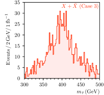
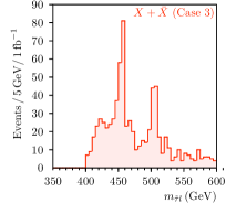
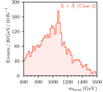
Figure 3: Left: NLSP stau invariant mass distribution for the case 3 of $X+\bar{X}$ messenger scenario. Center: $m_{\tilde{\tau}l}$ distribution. Right: Hemisphere invariant mass distribution.

To measure the neutralino masses $m_{\tilde{\chi}_{1,2}^{0}}$, we use the decay chain of $\tilde{\chi}_{1,2}^{0}\to\tilde{l}_{R}\,l_{n}\to\tilde{\tau}_{1}\,l_{n}\,l_{f}\,\tau$. Since mass difference between the lighter stau $\tilde{\tau}_{1}$ and the first two generation of right-handed sleptons $\tilde{l}_{R}$ are small in most of the cases we are interested in, we use the following approximation:

$$p_{\tilde{l}_{R}}=p_{\tilde{\tau}}+p_{l_{f}}+p_{\tau}\simeq p_{\tilde{\tau}_{1}}.$$ (3.5)

So we can measure the masses of the bino-like and wino-like neutralinos directly by taking the invariant mass of stau and $e$ or $\mu$ as illustrated in Figure 3. Although we can use the decay chain $\tilde{\chi}_{1,2}^{0}\to\tilde{\tau}_{1}\,\tau$ for the mass measurement of neutralinos, by this measurement the events with $e$ or $\mu$ are preferable because the momentum of $e$ or $\mu$ is less smeared than that of $\tau$. And we can confirm that the measured neutralinos are not higgsino-like one because of the large branching ratio for $\tilde{\chi}_{1,2}^{0}\to\tilde{l}_{R}\,l$.

In this scenario, it is expected that we can measure the masses of any kind of sparticles produced in each event. This is because the momentum of the arbitrary sparticle can be reconstructed by the momenta of the stau and the SM particles. So we can measure the mass of gluino and check the mass relation among all the gauginos in principle. Let us consider this issue in the rest of this subsection.

Although a large number of gluino are expected to be produced by the process $p\,p\to\tilde{g}\,\tilde{g},\,\tilde{g}\,\tilde{q}$ and the subsequent decay of squark, it is not always easy to distinguish gluino from squark in event-by-event level. Therefore we adopt the inclusive measurement of the invariant mass of produced sparticles. For this purpose, we use the hemisphere method suggested in [6, 36, 37]. In this method, we sort the clusters into two hemispheres in each event according to the following algorithm.

1. We pick all the jets with $p_{T}>50\,\mathrm{GeV}$, $|\eta|<2$, leptons with $p_{T}>15\,\mathrm{GeV}$, $|\eta|<3$ and two staus in each event. We use them as the clusters which compose two hemispheres corresponding to the pair-produced sparticles.

2. We define the initial hemisphere axes $p_{\text{hemi}}^{(i)}$ $(i=1,2)$ by the momentum of two clusters. $p_{\text{hemi}}^{(1)}$ is defined as the momentum of the highest $p_{T}$ cluster. And $p_{\text{hemi}}^{(2)}$ corresponds to the momentum of the cluster which has the largest value of $p_{T}\times\Delta R$ where $\Delta R\equiv\sqrt{\Delta\eta^{2}+\Delta\phi^{2}}$. Here $\Delta\eta\equiv\eta^{(1)}-\eta^{(2)}$, $\Delta\phi\equiv\phi^{(1)}-\phi^{(2)}$ and $\phi$ is the azimuthal angle of the cluster.

3. The cluster with momentum $p$ is belonging to the hemisphere 1 if it satisfies

   $$d(p,p_{\text{hemi}}^{(1)})<d(p,p_{\text{hemi}}^{(2)})$$ (3.6)

   and vise versa. Here $d(p_{j},p_{\text{hemi}}^{(i)})$ is the Lund distance measure between the clusters with momentum $p_{j}$ and $p_{\text{hemi}}^{(i)}$, and it is defined by

   $$d(p_{j},p_{\text{hemi}}^{(i)})=(E_{\text{hemi}}^{(i)}-|\bm{p}_{\text{hemi}}^{(i)}|\cos\theta_{ij})\frac{E_{\text{hemi}}^{(i)}}{(E_{\text{hemi}}^{(i)}+E_{j})^{2}}$$ (3.7)

   where $\theta_{ij}$ is the angle between $\bm{p}_{j}$ and $\bm{p}_{\text{hemi}}^{(i)}$.

4. We redefine the hemisphere axis $p_{\text{hemi}}^{(i)}$ as the sum of the momenta of the clusters which belong to the hemisphere $i$.

5. We repeat the step 3 and 4 until the classification of hemisphere converges.

After this algorithm, we can obtain the invariant mass distribution of each hemisphere $m_{\text{hemi}}^{2}=p_{\text{hemi}}^{2}$. If the assignment of hemisphere agrees with the true hemisphere, $m_{\text{hemi}}$ corresponds to the mass of the pair produced sparticle. Since the true hemisphere should contain exactly one stau, we reject the event where two staus are contained in one of the hemispheres.

Using this algorithm, we illustrate the distribution of $m_{\text{hemi}}$ in Figure 3. We can see from this figure that both gluino and squark have masses around $1000\,\mathrm{GeV}$ and the mass relation $m_{\tilde{W}}:m_{\tilde{g}}\sim 1:2$ can be checked.

3.2 Low luminosity analysis

In order to catch the features in the other cases of $X+\bar{X}$ messenger scenario and of $Q+\bar{Q}$ messenger scenario, we discuss the several analyses which can be done in the LHC with comparatively low luminosity.

Figure 4: Decay chains which we use for the analysis in this paper. $\tilde{\chi}_{2}^{0}$ decays to $\tilde{\chi}_{1}^{0}$ via the off-shell slepton in the case 1. In the case 2, $\tilde{\chi}_{2}^{0}$ decays to on-shell slepton and we label the leptons which come from the decay of $\tilde{\chi}_{2}^{0}$ and $\tilde{l}_{R}$ as $l_{n}$ and $l_{f}$, respectively.

Since we are interested in the measurement related to the masses of the bino and wino, we make use of the characteristic decay modes of these particles. As noted in the comment of feature 2, for $X+\bar{X}$ messenger scenario, the leptonic decay of wino-like neutralino $\tilde{\chi}_{2}^{0}$ to the lightest bino-like neutralino $\tilde{\chi}_{1}^{0}$ through on-shell or off-shell slepton $\tilde{l}_{R}$ is useful, which are illustrated in Figure 4.

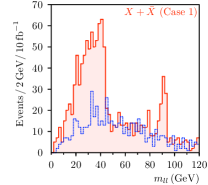
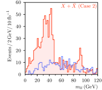
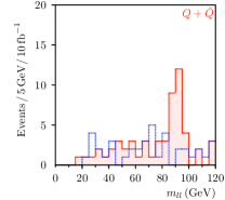
Figure 5: Dilepton invariant mass $m_{ll}$ distributions for $10\,\mathrm{fb}^{-1}$ of each model points. The bins illustrated by the dotted line represents the similar distribution using the opposite-sign and different flavor dileptons ($e^{+}\,\mu^{-}+\mu^{+}\,e^{-}$).

First, we consider the invariant mass of a pair of leptons coming from the decay of $\tilde{\chi}_{2}^{0}$. As can be seen from Table 2, in the $X+\bar{X}$ messenger scenario, a large number of $\tilde{\chi}_{2}^{0}$ is expected to be produced via the decay of left-handed squark $\tilde{q}_{L}$. We use a dilepton with opposite-sign and same-flavor ($e^{+}\,e^{-}+\mu^{+}\,\mu^{-}$) for making the invariant mass and the distribution shown in Figure 5 is obtained. In this figure, the background is estimated by taking the similar invariant mass of dilepton with opposite-sign and different-flavor ($e^{+}\,\mu^{-}+\mu^{+}\,e^{-}$). Here, in order to reduce the SM background, we impose following event cuts by using the transverse momenta $p_{T}$ [5]

• $p_{T}^{(1)}>100\,\mathrm{GeV}$ and $p_{T}^{(2,3,4)}>50\,\mathrm{GeV}$

• $M_{\text{eff}}\equiv p_{T}^{(1)}+p_{T}^{(2)}+p_{T}^{(3)}+p_{T}^{(4)}+E_{T}^{\text{miss}}>400\,\mathrm{GeV}$

• $E_{T}^{\text{miss}}>\mathop{\operator@font max}\limits\{100\,\mathrm{GeV},0.2M_{\text{eff}}\}$

• Two isolated leptons with $p_{T}^{e}>20\,\mathrm{GeV}$ and $p_{T}^{\mu}>5\,\mathrm{GeV}$

where $p_{T}^{(i)}$ means the $i$-th largest $p_{T}$ of the jet in each event and $E_{T}^{\text{miss}}=\sqrt{(p_{x}^{\text{miss}})^{2}+(p_{y}^{\text{miss}})^{2}}$. Since the SM background is reduced successfully after these cut, we generate only events of sparticle production for our simulation [5].

We can see the rather small maximum value of invariant mass for both cases of the $X+\bar{X}$ scenario in Figure 5, which is caused by the feature 2, namely, $m_{\tilde{B}}\sim m_{\tilde{W}}$. Actually, the maximum value of invariant mass allowed by kinematics is given as

$$m_{ll}^{\mathop{\operator@font max}\limits}[\text{Case 1}]=m_{\tilde{\chi}_{2}^{0}}-m_{\tilde{\chi}_{1}^{0}}$$ (3.8)

in region 1, and

$$(m_{ll}^{\mathop{\operator@font max}\limits}[\text{Case 2}])^{2}=m_{\tilde{\chi}_{2}^{0}}^{2}\left(1-\frac{m_{\tilde{l}_{R}}^{2}}{m_{\tilde{\chi}_{2}^{0}}^{2}}\right)\left(1-\frac{m_{\tilde{\chi}_{1}^{0}}^{2}}{m_{\tilde{l}_{R}}^{2}}\right)$$ (3.9)

in region 2, which result in rather small maximum value of the invariant mass calculated as

$$m_{ll}^{\mathop{\operator@font max}\limits}[\text{Case 1}]=44\,\mathrm{GeV},\qquad m_{ll}^{\mathop{\operator@font max}\limits}[\text{Case 2}]=47\,\mathrm{GeV}.$$ (3.10)

Unfortunately, the smallness of $m_{ll}^{\mathop{\operator@font max}\limits}$ does not always mean the smallness of the mass splitting between the bino and wino. For the case 2, if one of the relations $m_{\tilde{B}}\sim m_{\tilde{l}}$ and $m_{\tilde{l}}\sim m_{\tilde{W}}$ is satisfied, the maximum value of the invariant mass becomes small.

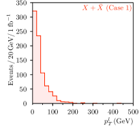
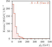
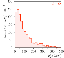
Figure 6: $p_{T}$ distributions of leptons emitted from sparticle decays. Each graph corresponds to $1\,\mathrm{fb}^{-1}$ for the case 1 of $X+\bar{X}$ scenario (left), $1\,\mathrm{fb}^{-1}$ for the case 2 of $X+\bar{X}$ scenario (center) and $10\,\mathrm{fb}^{-1}$ for $Q+\bar{Q}$ scenario (right).

To check that the mass difference between $\tilde{\chi}_{1}^{0}$ and $\tilde{\chi}_{2}^{0}$ is small in $X+\bar{X}$ scenario, we examine the $p_{T}$ distribution of leptons which come from the decay shown in Figure 4. Since the magnitude of $p_{T}$ of produced particles is strongly dependent on the mass difference among the sparticles, this can be a good signal to distinguish these scenarios. We can see from Figure 6 that these leptons have relatively small $p_{T}$ in the $X+\bar{X}$ scenario and large $p_{T}$ in the $Q+\bar{Q}$ scenario. These are caused by $m_{\tilde{B}}\sim m_{\tilde{W}}$ in the $X+\bar{X}$ scenario and $m_{\tilde{B}}\ll m_{\tilde{W}}$ in the $Q+\bar{Q}$ scenario.

Even in the models with the GUT relation for the gaugino masses, such a small value of $m_{ll}^{\mathop{\operator@font max}\limits}$ is possible if the gaugino mass scale is small. But such lighter gluino can be distinguished from heavier gluino in $X+\bar{X}$ messenger scenario by measuring the cross section and/or by the $m_{T2}$ method. As a reference model, we adopt the minimal supergravity (mSUGRA) model with parameters $m_{1/2}=150\,\mathrm{GeV}$, $m_{0}=750\,\mathrm{GeV}$, $A_{0}=-100\,\mathrm{GeV}$, $\tan\beta=10$ and $\mathrm{sgn}\,(\mu)=+1$. As shown later, though the distributions of $m_{ll}$ and $p_{T}$ in the reference model are similar to those of $X+\bar{X}$ messenger scenario in Figure 5 and 6, the distribution of $m_{T2}$ and the cross section become much different from those of $X+\bar{X}$ messenger scenario. Let us remind the $m_{T2}$ method [29, 30, 31]. When we consider the production process of sparticle pair which decay into a pair of the NLSPs and a pair of the SM particles, we can make use of the $m_{T2}$ variable defined by

$$m_{T2}(M_{\text{test}})\equiv\mathop{\operator@font min}\limits_{\bm{p}_{T}^{\text{miss}}=\mathop{\mathchoice{\textstyle\sum@}{\textstyle\sum@}{\scriptstyle\sum@}{\scriptscriptstyle\sum@}}\limits_{i}\bm{p}_{T}^{\chi(i)}}\left[\mathop{\operator@font max}\limits\left\{m_{T}(\overrightarrow{p}_{T}^{\text{vis}(1)},\overrightarrow{p}_{T}^{\chi(1)}),m_{T}(\overrightarrow{p}_{T}^{\text{vis}(2)},\overrightarrow{p}_{T}^{\chi(2)})\right\}\right].$$ (3.11)

Here $\overrightarrow{p}_{T}$ is a $(2+1)$-dimensional vector, $\overrightarrow{p}_{T}\equiv(E_{T},\bm{p}_{T})$, and $p_{T}^{\text{vis}(i)}$ is the transverse momentum for the emitted observed particles. $m_{T}$ is given by

$$m_{T}^{2}(\overrightarrow{p}_{T}^{\text{vis}},\overrightarrow{p}_{T}^{\chi})\equiv(\overrightarrow{p}_{T}^{\text{vis}}+\overrightarrow{p}_{T}^{\chi})^{2}=m_{\text{vis}}^{2}+M_{\text{test}}^{2}+2(E_{T}^{\text{vis}}\cdot E_{T}^{\chi}-\bm{p}_{T}^{\text{vis}}\cdot\bm{p}_{T}^{\chi})$$ (3.12)

where $E_{T}^{\text{vis}}\equiv\sqrt{m_{\text{vis}}^{2}+|\bm{p}^{\text{vis}}_{T}|^{2}}$ and $E_{T}^{\chi}\equiv\sqrt{M_{\text{test}}^{2}+|\bm{p}^{\chi}_{T}|^{2}}$.

Now we consider the process $p\,p\to\tilde{q}\,\tilde{q}\to\tilde{\chi}_{1}^{0}\,q\,\tilde{\chi}_{1}^{0}\,q$. In this process, $m_{\text{vis}}^{(1)}\simeq m_{\text{vis}}^{(2)}\simeq 0$ and the maximum value of $m_{T2}$ is given by

$$m_{T2}^{\mathop{\operator@font max}\limits}(M_{\text{test}})=\frac{m_{\tilde{q}}^{2}-m_{\tilde{\chi}_{1}^{0}}^{2}}{2m_{\tilde{q}}}+\sqrt{\left(\frac{m_{\tilde{q}}^{2}-m_{\tilde{\chi}_{1}^{0}}^{2}}{2m_{\tilde{q}}}\right)^{2}+M_{\text{test}}^{2}}$$ (3.13)

as a function of the test mass $M_{\text{test}}$. Therefore, we can obtain the rough value of the colored sparticle masses by this analysis.

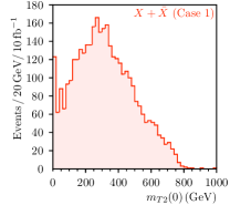
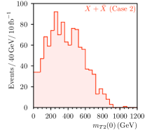
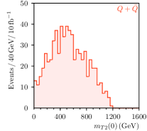
Figure 7: $m_{T2}$ distributions for $M_{\text{test}}=0$.

For the analysis of $m_{T2}$, we use the event cuts

• Two jets with $p_{T}>100\,\mathrm{GeV}$

• $M_{\text{eff}}\equiv p_{T}^{(1)}+p_{T}^{(2)}+E_{T}^{\text{miss}}>400\,\mathrm{GeV}$

• $E_{T}^{\text{miss}}>\mathop{\operator@font max}\limits\{100\,\mathrm{GeV},0.2M_{\text{eff}}\}$

• No lepton

instead of the usual cut for the SM events introduced above. Since (3.13) is satisfied for any fixed value of $M_{\text{test}}$, here we set $M_{\text{test}}=0$ for our analysis. Then (3.13) becomes the following simple form:

$$m_{T2}^{\mathop{\operator@font max}\limits}(0)=\frac{m_{\tilde{q}}^{2}-m_{\tilde{\chi}_{1}^{0}}^{2}}{m_{\tilde{q}}}$$ (3.14)

for the process of squark pair production. The distribution of this quantity is shown in Figure 7. If the mass of the LSP is very small compared with the mass of squark, we can interpret $m_{T2}^{\mathop{\operator@font max}\limits}(0)$ as the mass scale of squark. In fact, this is the case for $Q+\bar{Q}$ messenger scenario. However, the mass hierarchy of sparticles is small in $X+\bar{X}$ messenger scenario and the effect of $m_{\tilde{\chi}_{1}^{0}}$ is non-negligible. The theoretical values of $m_{T2}^{\mathop{\operator@font max}\limits}(0)$ are

$$m_{T2}^{\mathop{\operator@font max}\limits}(0)[\text{Case 1}]=844\,\mathrm{GeV},\qquad m_{T2}^{\mathop{\operator@font max}\limits}(0)[\text{Case 2}]=904\,\mathrm{GeV},$$ (3.15)

here we approximate $m_{\tilde{q}}=1000$ GeV for the case 1 and $m_{\tilde{q}}=1100$ GeV for the case 2. By this analysis, we can obtain the evidence of milder hierarchy between the masses of $\chi_{2}^{0}$ and colored sparticle if we know $m_{\tilde{\chi}_{2}^{0}}\simeq 500\,\mathrm{GeV}$. Unfortunately, we do not find the scale of $m_{\tilde{\chi}_{2}^{0}}$ by the analysis in this subsection and it needs further detailed analysis.

In the reference model, the distributions $m_{ll}$, $p_{T}$ and $m_{T2}$ are represented in Figure 8. The distribution of $m_{T2}$ is much different from those in Figure 7, although the distribution of $m_{ll}$ and $p_{T}$ is similar to those of $X+\bar{X}$ messenger scenario in Figure 5 and 6. And the cross section becomes much larger than in $X+\bar{X}$ scenario. Since the distribution of $m_{T2}$ and the cross section in $X+\bar{X}$ messenger scenario show the much larger mass scale of the colored particle than the gluino mass obtained by the GUT relation, it is suggested that the GUT relation is not satisfied.

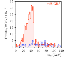
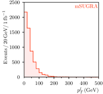
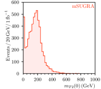
Figure 8: The measurements for the mSUGRA model point, where $m_{1/2}=150\,\mathrm{GeV}$, $m_{0}=750\,\mathrm{GeV}$, $A_{0}=-100\,\mathrm{GeV}$, $\tan\beta=10$ and $\mathrm{sgn}\,(\mu)=+1$. Left: Dilepton invariant mass $m_{ll}$ distribution. The bins illustrated by the dotted line represents the similar distribution using the opposite-sign and different flavor dileptons ($e^{+}\,\mu^{-}+\mu^{+}\,e^{-}$). Center: $p_{T}$ distribution of leptons emitted from sparticle decays. Right: $m_{T2}$ distribution for $M_{\text{test}}=0$.

3.3 $X+\bar{X}$ messenger scenario (Case 1, 2: neutralino NLSP)

In the cases 1 and 2 of $X+\bar{X}$ messenger scenario, the neutralino is the NLSP and we focus on the decay chain shown in Figure 4. Although these two cases give similar signals, the decay modes of the wino-like neutralino $\tilde{\chi}_{2}^{0}$ are different. In the case 1, $\tilde{\chi}_{2}^{0}$ undergoes three-body decay through off-shell slepton, while $\tilde{\chi}_{2}^{0}$ decays to the right-handed slepton $\tilde{l}_{R}$, which decays to $\tilde{\chi}_{1}^{0}$ subsequently, in the case 2. As seen in the previous section, the small values of $m_{ll}^{\rm max}$ and $p_{T}^{l}$ indicate that $m_{\tilde{\chi}_{2}^{0}}-m_{\tilde{\chi}_{1}^{0}}$ is small, but this may not mean that $m_{\tilde{\chi}_{2}^{0}}\sim m_{\tilde{\chi}_{1}^{0}}$ because the possibility may be still alive that the absolute value of the neutralino mass scale is small. In order to reject the possibility, we try to show the relation $m_{\tilde{\chi}_{2}^{0}}\sim m_{\tilde{\chi}_{1}^{0}}$ by measuring the invariant mass $m_{jl(u)}$ of a jet emitted from the squark $\tilde{q}$ and one of two leptons in the decay of $\tilde{\chi}_{2}^{0}$, although the large luminosity is required for this analysis. Since there are two leptons in each event, we include two invariant masses $m_{jl(u)}$ for each event in the distribution. In the case 1, the maximum value of $m_{jl(u)}$ is obtained as

$$(m_{jl(u)}^{\mathop{\operator@font max}\limits}[\text{Case 1}])^{2}=m_{\tilde{q}}^{2}\left(1-\frac{m_{\tilde{\chi}_{2}^{0}}^{2}}{m_{\tilde{q}}^{2}}\right)\left(1-\frac{m_{\tilde{\chi}_{1}^{0}}^{2}}{m_{\tilde{\chi}_{2}^{0}}^{2}}\right),$$ (3.16)

which is predicted to be 392 GeV for $m_{\tilde{q}}=1000\,\mathrm{GeV}$. Note that this predicted value is much smaller than $m_{T2}^{\rm max}(0)\sim 844$ GeV. This indicates that $m_{\tilde{\chi}_{2}^{0}}\sim m_{\tilde{\chi}_{1}^{0}}$ unless $m_{\tilde{q}}\sim m_{\tilde{\chi}_{2}^{0}}$. Note that in the case 2, there are two kinds of leptons in the decay because there is an on-shell slepton $\tilde{l}_{R}$ produced by the decay of $\tilde{\chi}_{2}^{0}$. Here we label two leptons emitted from $\tilde{\chi}_{2}^{0}$ and $\tilde{l}_{R}$ as “near”-lepton $l_{n}$ and “far”-lepton $l_{f}$, respectively, as shown in Figure 4. Since we cannot distinguish $l_{n}$ with $l_{f}$ in event-by-event level, we consider the quantity

$$m_{jl(u)}\equiv m_{jl_{n}}\cup m_{jl_{f}}$$ (3.17)

suggested by [38, 39]. $m_{jl_{n}}$($m_{jl_{f}}$) means the invariant mass of a jet emitted from squark $\tilde{q}$ and a lepton $l_{n}$($l_{f}$). Then $m_{jl(u)}$ gives a combined distribution of $m_{jl_{n}}$ and $m_{jl_{f}}$. The important point is that the analysis is completely the same as in the case 1, and we do not have to distinguish $l_{n}$ and $l_{f}$ at event-by-event level. The maximum value of the distribution of $m_{jl(u)}$ becomes

$$\mathop{\operator@font max}\limits\{m_{jl_{n}}^{\mathop{\operator@font max}\limits},m_{jl_{f}}^{\mathop{\operator@font max}\limits}\},$$ (3.18)

where

$$(m_{jl_{n}}^{\mathop{\operator@font max}\limits})^{2}=m_{\tilde{q}}^{2}\left(1-\frac{m_{\tilde{\chi}_{2}^{0}}^{2}}{m_{\tilde{q}}^{2}}\right)\left(1-\frac{m_{\tilde{l}_{R}}^{2}}{m_{\tilde{\chi}_{2}^{0}}^{2}}\right)$$ (3.19)

and

$$(m_{jl_{f}}^{\mathop{\operator@font max}\limits})^{2}=m_{\tilde{q}}^{2}\left(1-\frac{m_{\tilde{\chi}_{2}^{0}}^{2}}{m_{\tilde{q}}^{2}}\right)\left(1-\frac{m_{\tilde{\chi}_{1}^{0}}^{2}}{m_{\tilde{l}_{R}}^{2}}\right).$$ (3.20)

In the case 2, $m_{jl(u)}^{\mathop{\operator@font max}\limits}$ is predicted to be 369 GeV because $m_{jl_{n}}^{\mathop{\operator@font max}\limits}=262$ GeV and $m_{jl_{f}}^{\mathop{\operator@font max}\limits}=369$ GeV for $m_{\tilde{q}}=1150\,\mathrm{GeV}$. Again, this predicted value is much smaller than $m_{T2}^{\rm max}(0)\sim 904$ GeV, and it indicates that $m_{\tilde{\chi}_{2}^{0}}\sim m_{\tilde{\chi}_{1}^{0}}$ because $m_{jl_{n}}^{\mathop{\operator@font max}\limits}\ll m_{T2}^{\rm max}(0)$ means $m_{\tilde{\chi}_{2}^{0}}\sim m_{\tilde{l}_{R}}$ and $m_{jl_{f}}^{\mathop{\operator@font max}\limits}\ll m_{T2}^{\rm max}(0)$ means $m_{\tilde{\chi}_{1}^{0}}\sim m_{\tilde{l}_{R}}$ unless $m_{\tilde{q}}\sim m_{\tilde{\chi}_{2}^{0}}$. Therefore, if $m_{jl(u)}^{\rm max}$ is much smaller than $m_{T2}^{\rm max}(0)$, $m_{\tilde{\chi}_{2}^{0}}\sim m_{\tilde{\chi}_{1}^{0}}$ can be shown.

In our simulation, we impose the cuts for the standard model background as in the section 3.2 and use the dilepton whose invariant mass $m_{ll}$ is less than $50\,\mathrm{GeV}$ and a jet with $p_{T}$ larger than $100\,\mathrm{GeV}$. There are, however, many background of jets coming from other decays of colored sparticles, such as $\tilde{g}\to\tilde{t}_{1}\,\bar{t}\to\tilde{\chi}_{2}^{+}\,b\,\bar{t}$. To reduce these background, we impose another event cut that there is no $b$-tagged jet in each event. Here we assume $60\%$ tagging efficiency of $b$-jet. Then we make two invariant masses $m_{jl_{i}}$ ($i=1,2$) for all the possible jets in each event. And we choose a jet which minimizes $\mathop{\operator@font max}\limits\{m_{jl_{1}},m_{jl_{2}}\}$ among these jets. In this way we can obtain the distribution of $m_{jl(u)}$ which consists of the combined distribution of $m_{jl_{1}}$ and $m_{jl_{2}}$. The above predicted values are roughly consistent with the measured values obtained from Figure 9.

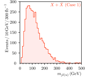
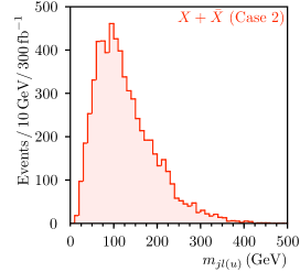
Figure 9: $m_{jl(u)}$ distributions for $300\,\mathrm{fb}^{-1}$ of the case 1 (left) and case 2 (right) of $X+\bar{X}$ scenario.

Note that in the case 1, taking account of three relations (3.8), (3.14) and (3.16) together, we can obtain the masses of squark $\tilde{q}$ and neutralinos $\tilde{\chi}_{1,2}^{0}$, in principle. We will return to this point in the end of this subsection.

In order to determine the mass spectrum of sparticles in the case 2, more measurements are needed. As suggested by [39], $\mathop{\operator@font min}\limits\{m_{jl_{n}}^{\mathop{\operator@font max}\limits},m_{jl_{f}}^{\mathop{\operator@font max}\limits}\}$ can be obtained from the distribution of $m_{jl(u)}$ by observing the structure with the intermediate endpoints in the case 2. Actually the predicted value roughly agrees with the measured value in Figure 9.

Although we do not know which of the two measured endpoints of $m_{jl(u)}$ in the case 2 corresponds to $m_{jl_{n}}$ ($m_{jl_{f}}$), it is shown in [39] that we can determine the masses of neutralinos without ambiguity by introducing the quantity

$$m_{jl(s)}^{2}\equiv m_{jl_{n}}^{2}+m_{jl_{f}}^{2}.$$ (3.21)

The maximum value of this quantity is obtained as

$$(m_{jl(s)}^{\mathop{\operator@font max}\limits}[\text{Case 2}])^{2} =(m_{jl_{n}}^{\mathop{\operator@font max}\limits})^{2}+\frac{m_{\tilde{l}_{R}}^{2}}{m_{\tilde{\chi}_{2}^{0}}^{2}}(m_{jl_{f}}^{\mathop{\operator@font max}\limits})^{2}$$

$$=m_{\tilde{q}}^{2}\left(1-\frac{m_{\tilde{\chi}_{2}^{0}}^{2}}{m_{\tilde{q}}^{2}}\right)\left(1-\frac{m_{\tilde{\chi}_{1}^{0}}^{2}}{m_{\tilde{\chi}_{2}^{0}}^{2}}\right).$$ (3.22)

in the case 2. Then we impose a similar event selection as in the previous one and make an invariant mass by a dilepton with $m_{ll}<50\,\mathrm{GeV}$ and a jet with $p_{T}>100\,\mathrm{GeV}$. Among all the possible choice of a jet, we pick the one which minimizes $m_{jl(s)}$ in each events. And the result of simulation is shown in Figure 10, whereas the theoretical value is calculated as

$$m_{jl(s)}^{\mathop{\operator@font max}\limits}[\text{Case 2}]=442\,\mathrm{GeV}.$$ (3.23)

From these quantities, we can obtain the neutralino masses without any ambiguity in the case 2 [39]. By denoting that

$$A\equiv m_{ll}^{\mathop{\operator@font max}\limits},\quad B\equiv\mathop{\operator@font max}\limits\{m_{jl_{n}}^{\mathop{\operator@font max}\limits},m_{jl_{f}}^{\mathop{\operator@font max}\limits}\},\quad C\equiv\mathop{\operator@font min}\limits\{m_{jl_{n}}^{\mathop{\operator@font max}\limits},m_{jl_{f}}^{\mathop{\operator@font max}\limits}\},\quad D\equiv m_{jl(s)}^{\mathop{\operator@font max}\limits},$$ (3.24)

the masses of neutralinos are written as

$$m_{\tilde{\chi}_{1}^{0}}[\text{Case 2}]=\frac{A\sqrt{(D^{2}-B^{2})(D^{2}-C^{2})}}{B^{2}+C^{2}-D^{2}},\qquad m_{\tilde{\chi}_{2}^{0}}[\text{Case 2}]=\frac{ABC}{B^{2}+C^{2}-D^{2}}.$$ (3.25)

Moreover, the squark mass is also obtained as

$$m_{\tilde{q}}[\text{Case 2}]=\frac{BC\sqrt{A^{2}+B^{2}+C^{2}-D^{2}}}{B^{2}+C^{2}-D^{2}}.$$ (3.26)

If we take $A=50\,\mathrm{GeV}$, $B=380\,\mathrm{GeV}$, $C=240\,\mathrm{GeV}$ and $D=440\,\mathrm{GeV}$, we obtain $m_{\tilde{\chi}_{1}^{0}}\simeq 490\,\mathrm{GeV}$, $m_{\tilde{\chi}_{2}^{0}}\simeq 540\,\mathrm{GeV}$ and $m_{\tilde{q}}\simeq 1130\,\mathrm{GeV}$, which are in good agreement with the real values in Table 3. The measured value of $m_{T2}^{\mathop{\operator@font max}\limits}(0)$ can be used to check the consistency.

We can also calculate the maximum value of $m_{jl(s)}$ for the case 1 as

$$m_{jl(s)}^{\mathop{\operator@font max}\limits}[\text{Case 1}] =m_{jll}^{\mathop{\operator@font max}\limits}[\text{Case 1}]=m_{\tilde{q}}^{2}\left(1-\frac{m_{\tilde{\chi}_{2}^{0}}^{2}}{m_{\tilde{q}}^{2}}\right)\left(1-\frac{m_{\tilde{\chi}_{1}^{0}}^{2}}{m_{\tilde{\chi}_{2}^{0}}^{2}}\right)$$

$$=m_{jl(u)}^{\mathop{\operator@font max}\limits}[\text{Case 1}].$$ (3.27)

where $m_{jll}$ means the invariant mass by the jet and dilepton. The first equality can be shown by the trivial relation

$$m_{jl(s)}^{2}=m_{jll}^{2}-m_{ll}^{2}$$ (3.28)

and the fact that $m_{jll}$ is maximized when $m_{ll}=0$ as long as $m_{\tilde{\chi}_{2}^{0}}/m_{\tilde{\chi}_{1}^{0}}<m_{\tilde{q}}/m_{\tilde{\chi}_{2}^{0}}$ is satisfied [38]. Let us determine the masses of squark and neutralinos $\tilde{\chi}_{1,2}^{0}$. For example, if we take $m_{ll}^{\mathop{\operator@font max}\limits}=45\,\mathrm{GeV}$, $m_{T2}^{\mathop{\operator@font max}\limits}(0)=800\,\mathrm{GeV}$ and $m_{jl(u)}^{\mathop{\operator@font max}\limits}=m_{jl(s)}^{\mathop{\operator@font max}\limits}=400\,\mathrm{GeV}$, then we can obtain $m_{\tilde{\chi}_{1}^{0}}\simeq 330\,\mathrm{GeV}$, $m_{\tilde{\chi}_{2}^{0}}\simeq 370\,\mathrm{GeV}$ and $m_{\tilde{q}}\simeq 920\,\mathrm{GeV}$ which are not far away from the real values in Table 2.

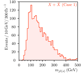
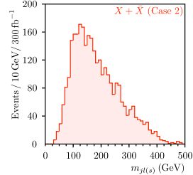
Figure 10: $m_{jl(s)}$ distributions for $300\,\mathrm{fb}^{-1}$ of the case 1 (left) and case 2 (right) of $X+\bar{X}$ scenario.

3.4 $Q+\bar{Q}$ messenger scenario

In $Q+\bar{Q}$ messenger scenario, we can see the dilepton signal if we collect a large number of events. The maximum value of $m_{ll}$ is given as

$$(m_{ll}^{\mathop{\operator@font max}\limits})^{2}=m_{\tilde{\chi}_{2}^{0}}^{2}\left(1-\frac{m_{\tilde{l}_{R}}^{2}}{m_{\tilde{\chi}_{2}^{0}}^{2}}\right)\left(1-\frac{m_{\tilde{\chi}_{1}^{0}}^{2}}{m_{\tilde{l}_{R}}^{2}}\right)$$ (3.29)

and the predicted value becomes

$$m_{ll}^{\mathop{\operator@font max}\limits}=569\,\mathrm{GeV}$$ (3.30)

in this model point. The result of simulation corresponding to $100\,\mathrm{fb}^{-1}$ is shown in Figure 11 and the measured value is consistent with the predicted value. Since $m_{ll}^{\mathop{\operator@font max}\limits}$ gives the lower bound of the mass of $\tilde{\chi}_{2}^{0}$, such a large value of $m_{ll}^{\mathop{\operator@font max}\limits}$ indicates the large $m_{\tilde{\chi}_{2}^{0}}$. In the section 3.2, we have already the mass scale of the heaviest colored particle, which is predicted as $1200\,\mathrm{GeV}$, by $m_{T2}$ analysis for the colored sparticle pair production. These signals mean that the mass ratio $m_{\tilde{\chi}_{2}^{0}}/m_{\tilde{g}}$ is roughly larger than 1/2, and therefore, the hierarchy between the gluino and wino masses is milder than that in the models with GUT relation.

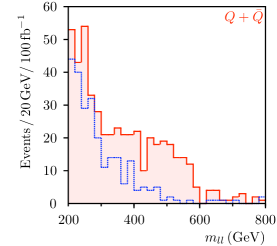
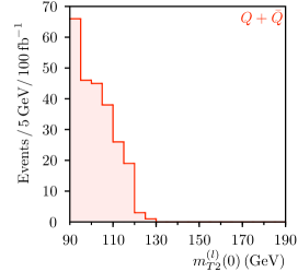
Figure 11: Left: Dilepton invariant mass $m_{ll}$ distribution for $100\,\mathrm{fb}^{-1}$ of $Q+\bar{Q}$ messenger scenario. The bins illustrated by the dotted line represents the similar distribution using the opposite-sign and different flavor dileptons ($e^{+}\,\mu^{-}+\mu^{+}\,e^{-}$). Right: leptonic $m_{T2}$ distribution for $100\,\mathrm{fb}^{-1}$ of $Q+\bar{Q}$ messenger scenario.

We can also use the $m_{T2}$ analysis for the right-handed slepton pair production, because the right-handed slepton also has a smaller mass compared with the other sparticles. Using the two leptons emitted from a pair of sleptons, we obtain the maximum value of $m_{T2}$ variable for $M_{\text{test}}=0\,\mathrm{GeV}$ as

$$m_{T2}^{(l)\mathop{\operator@font max}\limits}(0)=\frac{m_{\tilde{l}_{R}}^{2}-m_{\tilde{\chi}_{1}^{0}}^{2}}{m_{\tilde{l}_{R}}}$$ (3.31)

To select the process $p\,p\to\tilde{l}_{R}^{+}\,\tilde{l}_{R}^{-}\to\tilde{\chi}_{1}^{0}\,l^{+}\,\tilde{\chi}_{1}^{0}\,l^{-}$, we impose event cuts so that

• No jet with $p_{T}>20\,\mathrm{GeV}$

• Two leptons with $p_{T}^{l(1,2)}>50\,\mathrm{GeV}$ and no other leptons with $p_{T}^{l}>20\,\mathrm{GeV}$

• $E_{T}^{\text{miss}}>50\,\mathrm{GeV}$

• $p_{T}^{l(1)}+p_{T}^{l(2)}+E_{T}^{\text{miss}}>200\,\mathrm{GeV}$

• The invariant mass of two leptons is outside the region $80\,\mathrm{GeV}<m_{ll}<100\,\mathrm{GeV}$

are satisfied. Note that the last cut is imposed to suppress the SM background. Since the expected background coming from the SM events is leptonic decay of $W$ boson and $Z$ boson, we have to consider the $m_{T2}$ distribution for $WW$, $ZZ$, and $ZW$ production processes. For the process $p\,p\to W\,W\to l\,\nu\,l\,\nu$, it is obvious that

$$m_{T2}^{(l)}(0)\leq m_{W}$$ (3.32)

and the process $p\,p\to Z\,Z\to l\,l\,\nu\,\nu$ is rejected by the above cut. For $p\,p\to Z\,W\to l\,l\,l\,\nu$, this process will contribute to the $m_{T2}$ distribution if one of the leptons comes from $Z$ boson is missed to be detected. In that case,

$$m_{T2}^{(l)}(0)\leq\mathop{\operator@font max}\limits\{m_{Z},m_{W}\}=m_{Z}.$$ (3.33)

Therefore, the standard model background does not affect the measurement of $m_{T2}^{(l)\mathop{\operator@font max}\limits}(0)$ if $(m_{\tilde{l}_{R}}^{2}-m_{\tilde{\chi}_{2}^{0}}^{2})/m_{\tilde{l}_{R}}>m_{Z}$ is satisfied. We checked that these SM background can be negligible by producing the SM background from the $ZZ$, $WW$, and $ZW$ processes with the above cuts.

In the model point we are considering here, the maximum value of this $m_{T2}$ variable is given as

$$M\equiv m_{T2}^{(l)\mathop{\operator@font max}\limits}(0)=116\,\mathrm{GeV}$$ (3.34)

and the result is shown in Figure 11. Here we illustrate the distribution in the region $m_{T2}^{(l)}(0)\geq m_{Z}$, because the SM background is expected to be negligible only in this region.

The important relation $m_{\tilde{\chi}_{2}^{0}}\gg m_{\tilde{\chi}_{1}^{0}}$ can be obtained by the calculation as

$$\frac{m_{\tilde{\chi}_{2}^{0}}^{2}}{m_{\tilde{\chi}_{1}^{0}}}>\frac{m_{\tilde{\chi}_{2}^{0}}^{2}}{m_{\tilde{l}_{R}}}>\frac{m_{\tilde{\chi}_{2}^{0}}^{2}-m_{\tilde{l}_{R}}^{2}}{m_{\tilde{l}_{R}}}=\frac{(m_{ll}^{\mathop{\operator@font max}\limits})^{2}}{m_{T2}^{(l)\mathop{\operator@font max}\limits}(0)}\sim 2.8\,\mathrm{TeV},$$ (3.35)

where we use the measured values of $m_{ll}^{\mathop{\operator@font max}\limits}$ and $m_{T2}^{(l)\mathop{\operator@font max}\limits}(0)$.

It may be possible to measure the masses of $m_{\tilde{l}_{R}}$ and $m_{\chi_{1}^{0}}$ by the methods discussed in the papers [41, 42]. Here we do not discuss this issue further.

4 Discussion

Generically, multiple fields may play as the messenger fields. Actually, any vector-like fields $\Phi_{i}$ and $\bar{\Phi}_{i}$ ($i=1,\cdots,n$) can be the messenger fields if they have an interaction with the spurion field $S$ like $\kappa\Phi_{i}\bar{\Phi}_{i}S$. Here the $F$ component of $S$ has non-vanishing VEV $F_{S}$ which breaks the SUSY. Naively, they have the same order of the contribution to the SUSY breaking parameters if the coefficients $\kappa_{i}\sim c_{i}m_{\Phi_{i}}/\Lambda$ where $\Lambda$ is the cutoff. Namely, the scale $\Lambda_{\Phi}\equiv F_{\Phi_{i}}/m_{\Phi_{i}}\sim\alpha_{i}F_{S}/\Lambda$ becomes independent of $i$ except the coefficients $c_{i}$ of the interactions $m_{\Phi_{i}}\Phi_{i}\bar{\Phi}_{i}S/\Lambda$. Because of the freedom of the $\mathcal{O}(1)$ coefficients, we have various possibilities for the sparticle spectrum. Indeed, any gaugino mass spectrum are possible by choosing the coefficients $c_{i}$. In this paper, we consider an extreme case, in which one of the coefficients becomes much larger than the others. This can often happen when the coefficients are the ratio of the $\mathcal{O}(1)$ coefficients $c_{i}=a_{i}/b_{i}$, where the $\mathcal{O}(1)$ coefficients $a_{i}$ and $b_{i}$ are determined randomly, for example, between 0 and 1. Since it is reasonable to expect that one of the $n$ coefficients of the denominator, which is noted as $b_{1}$, becomes $\mathcal{O}$($1/n$), the coefficient $c_{1}$ can be $\mathcal{O}$($n$). If $n\gg 1$, very large coefficient $c_{1}$ is realized. Moreover, if $b_{1}$ happens to be $\mathcal{O}(1/(10n))$, which requires 10% tuning, $c_{1}\sim\mathcal{O}(10n)$, and therefore, the messenger field $\Phi_{1}$ and $\bar{\Phi}_{1}$ can dominate the others. If $\mathop{\mathchoice{\textstyle\sum@}{\textstyle\sum@}{\scriptstyle\sum@}{\scriptscriptstyle\sum@}}\limits_{i}^{n}c_{i}\sim\mathcal{O}(100)$, then since the loop suppression is almost compensated by the summation of the coefficients, the contributions to the SUSY breaking parameters from the gauge mediation may become of the same order as those from the direct interactions between the spurion field and MSSM fields, for example, $Q^{\dagger}QS^{\dagger}S/\Lambda^{2}$ in the Kähler potential. $n$ can be much larger than 1, for example, in the anomalous $U(1)$ GUT scenario, there are many vector-like fields which have non-trivial charges under the standard gauge group and can be the messenger fields. There are 23 vector-like pairs in the $SO(10)$ model [17, 20], 47 pairs in the $E_{6}$ model [18], 38 pairs in the simpler $E_{6}$ model [19] except the MSSM Higgs doublet pair.

In this paper, we consider the several cases in which one vector-like messenger field dominates the others. Note that although we have chosen $X+\bar{X}$ or $Q+\bar{Q}$ as the messenger field in order to obtain non-vanishing gaugino masses, other choices become possible if the small but non-zero contributions from the other vector-like fields are taken into account.

If there are multiple messengers $\Phi_{i}$ and $\bar{\Phi}_{i}$ ($i=1,\cdots,n$) which has the same quantum numbers, $D$-term contribution of $U(1)_{Y}$ hypercharge to the sfermion masses becomes important [40]. This contribution comes from one-loop Feynman graph and may not be negligible. The explicit formula is given by

$$\Delta m_{\tilde{f}}^{2}\sim\frac{1}{2}\mathop{\mathchoice{\textstyle\sum@}{\textstyle\sum@}{\scriptstyle\sum@}{\scriptscriptstyle\sum@}}\limits_{\Phi}\left(\frac{\alpha_{1}}{4\pi}\right)Y_{\tilde{f}}Y_{\Phi}\mathop{\mathchoice{\textstyle\sum@}{\textstyle\sum@}{\scriptstyle\sum@}{\scriptscriptstyle\sum@}}\limits_{i,j}\frac{|F_{\Phi_{ij}}|^{2}-|F_{\Phi_{ji}}|^{2}}{\mathop{\operator@font max}\limits\{(m_{\Phi_{i}})^{2},(m_{\Phi_{j}})^{2}\}},$$ (4.1)

where $F_{\Phi_{ij}}$ is a SUSY breaking mass mixing parameters (so called $B$ parameter) of the messenger fields in the unit in which the mass matrix of the messenger fields is diagonalized as

$$W_{\text{mess}}=m_{\Phi_{i}}\Phi_{i}\bar{\Phi}_{i}+\theta^{2}F_{\Phi_{ij}}\Phi_{i}\bar{\Phi}_{j}.$$ (4.2)

If the enhancement factor $c\gg\mathcal{O}(10^{2})$, then such contribution can be negligible.

5 Summary

In this paper, we investigated the LHC signatures of the generalized GMSB models with the messenger fields which do not respect $SU(5)$ GUT symmetry. Such a situation can be realized in the anomalous $U(1)$ GUTs in which the success of the gauge coupling unification can be explained although the mass spectrum of the vector-like fields do not respect $SU(5)$ GUT symmetry. The mass spectrum of sparticles become different from those in the usual GMSB whose messenger fields respect $SU(5)$ GUT symmetry. Especially, the gaugino masses do not satisfy the usual GUT relation and this feature is very important to distinguish these models by the LHC measurements. In principle, any mass pattern for the gaugino masses is possible in this generalized GMSB scenario. In this paper, only for simplicity, we examined the models with a pair of messenger fields which have quantum numbers of $X+\bar{X}$ or $Q+\bar{Q}$ and studied how to obtain the signatures of these models in the LHC. The gaugino mass relation becomes $m_{\tilde{B}}:m_{\tilde{W}}:m_{\tilde{g}}\sim 5:6:12$ for the $X+\bar{X}$ messenger model and $m_{\tilde{B}}:m_{\tilde{W}}:m_{\tilde{g}}\sim 1/5:6:12$ for the $Q+\bar{Q}$ messenger model. One of the interesting features of the both models is that the hierarchy between the colored particle masses and weakly charged particle masses becomes milder than the usual GMSB models because the messenger fields have bi-fundamental representation under $SU(3)_{C}\times SU(2)_{L}$. If we catch the scale of the wino mass in the LHC, we can roughly check this milder hierarchy by measuring $m_{T2}$ by which the order of the colored particle masses can be obtained. In $X+\bar{X}$ messenger scenario, the mass hierarchy between the bino and wino is very small, and it leads to the relatively soft $p_{T}$ distribution of leptons. On the other hand, the mass difference between the bino and wino is considerably large in $Q+\bar{Q}$ messenger scenario. Therefore very large $p_{T}$ distribution of leptons can be seen at the LHC.

The NLSP of $X+\bar{X}$ messenger scenario is the stau or neutralino. If the NLSP is the stau, we can check the mass relation of gauginos at the low-luminosity stage of the LHC and the deviation from the usual GUT relation can be obvious. If the NLSP is the neutralino, we can determine the bino-like and wino-like neutralino masses by the use of the end-point in the neutralino’s leptonic decay and of the $m_{T2}$ measurement.

In $Q+\bar{Q}$ messenger scenario, the leptonic $m_{T2}$ measurement is useful because the right-handed slepton remains light.

Since both scenarios predict very characteristic mass spectra, it is expected that we can distinguish these models from the models which satisfy the GUT relation.

Appendix A Two-loop RGE effects for the gaugino mass

There is a well-known feature in the softly broken SUSY models. Namely, by looking one-loop RGEs of gauge couplings and gaugino masses, one can see that their ratio obeys the following RGE.

$$\frac{d}{d\ln Q}\left(\frac{M_{a}}{\alpha_{a}}\right)=0.$$ (A.1)

Then, the gaugino masses in the GMSB model satisfy the relation

$$M_{1}:M_{2}:M_{3}\sim n_{1}\alpha_{1}:n_{2}\alpha_{2}:n_{3}\alpha_{3}$$ (A.2)

at any renormalization scale. But it should be noticed that (A.1) is satisfied only up to one-loop order, so the actual relation is deviated from (A.2) by two-loop order correction.

Let us estimate the effect of two-loop order RGE. The two-loop RGE of gauge couplings and gaugino masses are given by

$$\frac{d}{d\ln Q}\alpha_{a}^{-1}=-\frac{b_{a}}{2\pi}-\mathop{\mathchoice{\textstyle\sum@}{\textstyle\sum@}{\scriptstyle\sum@}{\scriptscriptstyle\sum@}}\limits_{b}\frac{B_{ab}}{8\pi^{2}}\alpha_{b}+\frac{c_{a}}{8\pi^{2}}\alpha_{t}$$ (A.3)

and

$$\frac{d}{d\ln Q}M_{a}=\frac{b_{a}}{2\pi}\alpha_{a}M_{a}+\frac{1}{8\pi^{2}}\alpha_{a}\left[\mathop{\mathchoice{\textstyle\sum@}{\textstyle\sum@}{\scriptstyle\sum@}{\scriptscriptstyle\sum@}}\limits_{b}B_{ab}\alpha_{b}(M_{a}+M_{b})+c_{a}\alpha_{t}(A-M_{a})\right],$$ (A.4)

neglecting the Yukawa coupling other than top quark component $\alpha_{t}\equiv y_{t}^{2}/4\pi^{2}$. Here, $A$ is defined by $A$-term $A_{t}\equiv Ay_{t}$. If there are no other vector-like particles below the mass scale of messenger field, $m_{\Phi}$, the coefficients $b_{a}$, $c_{a}$ and $B_{ab}$ are given as

$$(b_{1},b_{2},b_{3})=(33/5,1,-3),\qquad(c_{1},c_{2},c_{3})=(26/5,14/5,18/5)$$ (A.5)

and

$$\begin{pmatrix}B_{11}&B_{12}&B_{13}\\ B_{21}&B_{22}&B_{23}\\ B_{31}&B_{32}&B_{33}\end{pmatrix}=\begin{pmatrix}199/25&27/5&88/5\\ 9/5&25&24\\ 11/5&9&14\end{pmatrix}.$$ (A.6)

Then the deviation of RGE from (A.1) can be written as

$$\frac{d}{d\ln Q}\left(\frac{M_{a}}{\alpha_{a}}\right)=\mathop{\mathchoice{\textstyle\sum@}{\textstyle\sum@}{\scriptstyle\sum@}{\scriptscriptstyle\sum@}}\limits_{b}\frac{B_{ab}}{8\pi^{2}}\alpha_{b}M_{b}+\frac{c_{a}}{8\pi^{2}}\alpha_{t}A.$$ (A.7)

By using one-loop RGE for $A\equiv A_{t}y_{t}^{-1}$

$$\frac{d}{d\ln Q}A=\frac{3}{\pi}\alpha_{t}A+\mathop{\mathchoice{\textstyle\sum@}{\textstyle\sum@}{\scriptstyle\sum@}{\scriptscriptstyle\sum@}}\limits_{a}\frac{d_{a}}{4\pi}\alpha_{a}M_{a}+\mathcal{O}(\alpha^{2})$$ (A.8)

and one-loop part of (A.4), two-loop RGE (A.7) can be rewritten as

$$d\left(\frac{M_{a}}{\alpha_{a}}\right)=\frac{1}{4\pi}\mathop{\mathchoice{\textstyle\sum@}{\textstyle\sum@}{\scriptstyle\sum@}{\scriptscriptstyle\sum@}}\limits_{b}\frac{B_{ab}}{b_{b}}dM_{b}+\frac{c_{a}}{24\pi}\left(dA-\mathop{\mathchoice{\textstyle\sum@}{\textstyle\sum@}{\scriptstyle\sum@}{\scriptscriptstyle\sum@}}\limits_{b}\frac{d_{b}}{2b_{b}}dM_{b}\right)+\mathcal{O}(\alpha^{2})$$ (A.9)

where

$$(d_{1},d_{2},d_{3})=(26/15,6,32/3).$$ (A.10)

Therefore, integrating (A.9) from messenger mass scale $m_{\Phi}$ to $m_{Z}$, we can obtain the gaugino mass formula at the scale $m_{Z}$ including the two-loop effect. Because $A(m_{Z})\simeq A_{t}(m_{Z})$, $A(m_{\Phi})\simeq 0$ and $M_{a}(m_{Z})\simeq M_{a}\alpha_{a}^{-1}(m_{\Phi})\cdot\alpha_{a}(m_{Z})$ at one-loop order, this is expressed as

$$M_{a}\alpha_{a}^{-1}(m_{Z}) =M_{a}\alpha_{a}^{-1}(m_{\Phi})+\frac{c_{a}}{24\pi}A_{t}(m_{Z})$$

$$\qquad-\frac{1}{4\pi}\mathop{\mathchoice{\textstyle\sum@}{\textstyle\sum@}{\scriptstyle\sum@}{\scriptscriptstyle\sum@}}\limits_{b}\left(\frac{B_{ab}}{b_{b}}-\frac{c_{a}d_{b}}{12b_{b}}\right)M_{b}\alpha_{b}^{-1}(m_{\Phi})\Delta\alpha_{b},$$ (A.11)

where $\Delta\alpha_{a}\equiv\alpha_{a}(m_{\Phi})-\alpha_{a}(m_{Z})$. If we write $\Lambda_{\Phi}\equiv F_{\Phi}/m_{\Phi}$ and $r_{t}\equiv-4\pi A_{t}(m_{Z})/\Lambda_{\Phi}$, we finally obtain a following result.

$$M_{a}\alpha_{a}^{-1}(m_{Z})=\left[n_{a}-\frac{c_{a}}{24\pi}r_{t}-\mathop{\mathchoice{\textstyle\sum@}{\textstyle\sum@}{\scriptstyle\sum@}{\scriptscriptstyle\sum@}}\limits_{b}\frac{n_{b}}{4\pi}\left(\frac{B_{ab}}{b_{b}}-\frac{c_{a}d_{b}}{12b_{b}}\right)\Delta\alpha_{b}\right]\frac{\Lambda_{\Phi}}{4\pi}.$$ (A.12)

Since the order of $r_{t}$ and $\Delta\alpha_{a}$ are $\mathcal{O}(0.1)$ at most, two-loop contribution cannot become so large in the typical case, although it can becomes important if $n_{a}\ll 1$.

References

- [1] H. P. Nilles, “Supersymmetry, Supergravity And Particle Physics,” Phys. Rept. 110, 1 (1984).
- [2] H. E. Haber and G. L. Kane, “The Search For Supersymmetry: Probing Physics Beyond The Standard Model,” Phys. Rept. 117, 75 (1985).
- [3] S. P. Martin, “A Supersymmetry Primer,” arXiv:hep-ph/9709356.
- [4] G. Aad et al. [The ATLAS Collaboration], “Expected Performance of the ATLAS Experiment - Detector, Trigger and Physics,” arXiv:0901.0512 [hep-ex].
- [5] ATLAS collaboration, “ATLAS: Detector and physics performance technical design report. Volume 1,” CERN-LHCC-99-14 (1999), “ATLAS detector and physics performance. Technical design report. Vol. 2,” CERN-LHCC-99-15 (1999).
- [6] G. L. Bayatian et al. [CMS Collaboration], “CMS technical design report, volume II: Physics performance,” J. Phys. G 34 (2007) 995.
- [7] I. Hinchliffe, F. E. Paige, M. D. Shapiro, J. Soderqvist and W. Yao, “Precision SUSY measurements at CERN LHC,” Phys. Rev. D 55, 5520 (1997) [arXiv:hep-ph/9610544].
- [8] I. Hinchliffe and F. E. Paige, “Measurements in gauge mediated SUSY breaking models at LHC,” Phys. Rev. D 60, 095002 (1999) [arXiv:hep-ph/9812233].
- [9] H. Bachacou, I. Hinchliffe and F. E. Paige, “Measurements of masses in SUGRA models at CERN LHC,” Phys. Rev. D 62, 015009 (2000) [arXiv:hep-ph/9907518].
- [10] B. C. Allanach, C. G. Lester, M. A. Parker and B. R. Webber, “Measuring sparticle masses in non-universal string inspired models at the LHC,” JHEP 0009, 004 (2000) [arXiv:hep-ph/0007009].
- [11] B. K. Gjelsten, D. J. . Miller and P. Osland, “Measurement of SUSY masses via cascade decays for SPS 1a,” JHEP 0412, 003 (2004) [arXiv:hep-ph/0410303].
- [12] S. P. Martin, “Generalized messengers of supersymmetry breaking and the sparticle mass spectrum,” Phys. Rev. D 55, 3177 (1997) [arXiv:hep-ph/9608224].
- [13] P. Meade, N. Seiberg and D. Shih, “General Gauge Mediation,” Prog. Theor. Phys. Suppl. 177, 143 (2009) [arXiv:0801.3278 [hep-ph]].
- [14] D. Marques, “Generalized messenger sector for gauge mediation of supersymmetry breaking and the soft spectrum,” JHEP 0903, 038 (2009) [arXiv:0901.1326 [hep-ph]].
- [15] M. Dine and A. E. Nelson, “Dynamical supersymmetry breaking at low-energies,” Phys. Rev. D 48, 1277 (1993) [arXiv:hep-ph/9303230].
- [16] M. Dine, A. E. Nelson and Y. Shirman, “Low-Energy Dynamical Supersymmetry Breaking Simplified,” Phys. Rev. D 51, 1362 (1995) [arXiv:hep-ph/9408384].
- [17] N. Maekawa, “Neutrino masses, anomalous U(1) gauge symmetry and doublet-triplet splitting,” Prog. Theor. Phys. 106, 401 (2001) [arXiv:hep-ph/0104200].
- [18] N. Maekawa and T. Yamashita, “E(6) unification, doublet-triplet splitting and anomalous U(1)A symmetry,” Prog. Theor. Phys. 107, 1201 (2002) [arXiv:hep-ph/0202050].
- [19] N. Maekawa and T. Yamashita, “Simple E(6) unification with anomalous U(1)A symmetry,” Prog. Theor. Phys. 110, 93 (2003) [arXiv:hep-ph/0303207].
- [20] N. Maekawa, “Gauge coupling unification with anomalous U(1)A gauge symmetry,” Prog. Theor. Phys. 107, 597 (2002) [arXiv:hep-ph/0111205].
- [21] N. Maekawa and T. Yamashita, “Gauge coupling unification in GUT with anomalous U(1) symmetry,” Phys. Rev. Lett. 90, 121801 (2003) [arXiv:hep-ph/0209217].
- [22] B. C. Allanach, “SOFTSUSY: A C++ program for calculating supersymmetric spectra,” Comput. Phys. Commun. 143, 305 (2002) [arXiv:hep-ph/0104145].
- [23] C. Amsler et al. [Particle Data Group], “Review of particle physics,” Phys. Lett. B 667, 1 (2008).
- [24] H. K. Dreiner, S. Heinemeyer, O. Kittel, U. Langenfeld, A. M. Weber and G. Weiglein, “Mass Bounds on a Very Light Neutralino,” Eur. Phys. J. C 62, 547 (2009) [arXiv:0901.3485 [hep-ph]].
- [25] F. E. Paige, S. D. Protopopescu, H. Baer and X. Tata, “ISAJET 7.69: A Monte Carlo event generator for p p, anti-p p, and e+ e- reactions,” arXiv:hep-ph/0312045.
- [26] G. Corcella et al., “HERWIG 6.5: an event generator for Hadron Emission Reactions With Interfering Gluons (including supersymmetric processes),” JHEP 0101, 010 (2001) [arXiv:hep-ph/0011363].
- [27] G. Corcella et al., “HERWIG 6.5 release note,” arXiv:hep-ph/0210213.
- [28] E. Richter-Was, “AcerDET: A particle level fast simulation and reconstruction package for phenomenological studies on high p(T) physics at LHC,” arXiv:hep-ph/0207355.
- [29] C. G. Lester and D. J. Summers, “Measuring masses of semiinvisibly decaying particles pair produced at hadron colliders,” Phys. Lett. B 463, 99 (1999) [arXiv:hep-ph/9906349].
- [30] A. Barr, C. Lester and P. Stephens, “m(T2) : The Truth behind the glamour,” J. Phys. G 29, 2343 (2003) [arXiv:hep-ph/0304226].
- [31] A. J. Barr and C. Gwenlan, “The race for supersymmetry: using mT2 for discovery,” arXiv:0907.2713 [hep-ph].
- [32] G. Polesello and A. Rimoldi, “Reconstruction of quasi-stable charged sleptons in the ATLAS experiment,” ATLAS Internal Note ATL-MUON-99-06.
- [33] S. Ambrosanio, B. Mele, S. Petrarca, G. Polesello and A. Rimoldi, “Measuring the SUSY breaking scale at the LHC in the slepton NLSP scenario of GMSB models,” JHEP 0101, 014 (2001) [arXiv:hep-ph/0010081].
- [34] J. R. Ellis, A. R. Raklev and O. K. Oye, “Gravitino dark matter scenarios with massive metastable charged sparticles at the LHC,” JHEP 0610, 061 (2006) [arXiv:hep-ph/0607261].
- [35] A. Rajaraman and B. T. Smith, “Determining Spins of Metastable Sleptons at the Large Hadron Collider,” Phys. Rev. D 76, 115004 (2007) [arXiv:0708.3100 [hep-ph]].
- [36] S. Matsumoto, M. M. Nojiri and D. Nomura, “Hunting for the top partner in the littlest Higgs model with T-parity at the LHC,” Phys. Rev. D 75, 055006 (2007) [arXiv:hep-ph/0612249].
- [37] M. M. Nojiri, K. Sakurai, Y. Shimizu and M. Takeuchi, “Handling jets + missing channel using inclusive mT2,” JHEP 0810, 100 (2008) [arXiv:0808.1094 [hep-ph]].
- [38] M. Burns, K. T. Matchev and M. Park, “Using kinematic boundary lines for particle mass measurements and disambiguation in SUSY-like events with missing energy,” JHEP 0905, 094 (2009) [arXiv:0903.4371 [hep-ph]].
- [39] K. T. Matchev, F. Moortgat, L. Pape and M. Park, “Precise reconstruction of sparticle masses without ambiguities,” JHEP 0908, 104 (2009) [arXiv:0906.2417 [hep-ph]].
- [40] S. Dimopoulos and G. F. Giudice, “Multi-messenger theories of gauge-mediated supersymmetry breaking,” Phys. Lett. B 393, 72 (1997) [arXiv:hep-ph/9609344].
- [41] P. Konar, K. Kong, K. T. Matchev and M. Park, “Superpartner mass measurements with 1D decomposed MT2,” arXiv:0910.3679 [hep-ph].
- [42] K. T. Matchev and M. Park, “A general method for determining the masses of semi-invisibly decaying particles at hadron colliders,” arXiv:0910.1584 [hep-ph].