Price Trends in a Simplified Model of the Wealth Game

Abstract

We consider a simplified version of the Wealth Game, which is an agent-based financial market model with many interesting features resembling the real stock market. Market makers are not present in the game so that the majority traders are forced to reduce the amount of stocks they trade, in order to have a balance in the supply and demand. The strategy space is also simplified so that the market is only left with strategies resembling the decisions of optimistic or pessimistic fundamentalists and trend-followers in the real stock market. A dynamical phase transition between a trendsetters’ phase and a bouncing phase is discovered in the space of price sensitivity and market impact. Analysis based on a semi-empirical approach explains the phase transition and locates the phase boundary. A phase transition is also observed when the fraction of trend-following strategies increases, which can be explained macroscopically by matching the supply and demand of stocks.

I Introduction

A recent remarkable trend in the physics community is its engagement in interdisciplinary fields using physics-inspired techniques. Econophysics is one such area in which financial markets are simulated by agent-based models in much the same way as other many-body systems in statistical physics. The Minority Game (MG) Challet97 is an agent-based model based on the insight that agents making minority decisions in markets can take advantage of other agents. Due to its success in capturing the profit-seeking behavior of agents, it became the progenitor of a family of agent-based models Challet05 , which study various aspects of market behavior, such as volatility Savit99 , noise Cavagna99 , market-clearing mechanisms Jefferies01 , and anticipative strategies Andersen03 .

The market behavior depends on the way the agents evaluate their strategies when they make choices among them to take actions. In early versions of the minority games, agents evaluate their strategies using various virtual points or scores. Typical virtual point updating rules, such as those in the original MG Challet97 , evaluate the buying and selling decisions at a time step, regardless of the need to update the historical effects of the previous decisions. In other models, one-step expectations of the agents are considered, leading to the $-game Andersen03 . There are also market models with a mixture of trend-following and fundamentalist agents Marsili01 ; Demartino03 or markets with crossover regimes dominated by trend-following and fundamentalist strategies Lux99 ; Demartino04 . As pointed out in Yeung08 , these models do not reflect the history-dependent considerations of real market agents.

Improved versions of the minority games considered agents using virtual wealth to evaluate their strategies Challet08 . The Wealth Game (WG) Yeung08 was introduced to overcome this deficiency. Agents in WG evaluate their strategies by calculating their virtual wealth, that is, the wealth (including cash and stocks) that the strategies would bring were their recommendations completely adopted in history. The most significant advantage of this evaluation method can be seen when agents are allowed to make holding decisions (that is, decisions to take no buying or selling actions). In WG, the virtual wealth due to holding long (short) positions increases when stock prices are rising (dropping). On the other hand, virtual point updates in the original MG are neutral to holding positions. Tests with real market and artificial data confirm the versatility of wealth-based strategies Yeung08 ; Baek10 .

A consequence of using wealth-based strategies in WG is the emergence of price cycles through the self-organization of the different types of agents. This is both an important and interesting issue, since it sheds light on the formation and disappearance of bubbles and crashes in real financial markets. Giardina and Bouchaud considered a model with bubbles and crashes in the price trend of the market Giardina03 . The behavior was explained in terms of the interplay between the trend-following and fundamentalist behaviors of the agents, but the mechanism of the disappearance of this periodic phase remains an open issue. In WG, the roles of the trendsetters and fickle agents in sustaining the price cycles were explained, and the disappearance of the periodic phase was attributed to the failure of the trendsetters to gain wealth from the fickle agents. (The trendsetters are synonymous to the trend-followers in the literature, but are renamed trendsetters to emphasize their role in initiating the bubbles and crashes.) However, this picture assumes the presence of market makers, who manage to fulfill buy and sell orders irrespective of the order imbalance. This is not applicable to the stock market, since in the absence of market makers, the market clearing mechanism requires an exact matching of buy and sell orders. Consequently, not all agents can have their buying or selling orders fulfilled. Thus, the unfulfilled buyers (sellers) would repeat their bids (asks) step after step. This creates a much stronger tendency for the price to go monotonically upwards (downwards). The appearance of the periodic phase becomes questionable and, if it exists, its mechanism of formation and disappearance may not necessarily be the same.

In this paper, we study a simplified model of WG in the absence of market makers, focusing on the mechanism creating and destroying the cycles of bubbles and crashes. We will adopt a minimalist approach, and consider the simple but essential elements that contribute to the studied mechanism. It turns out that with trend-followers and fundamentalists of memory size 2 being the two main groups of investors, the price dynamics already exhibits many interesting features. (The fundamentalists are further divided into optimistic and pessimistic subgroups.) On one hand, these groups are inclusive enough to represent the attitudes of most investors, and on the other hand, simple enough to enable convenient analyses. Despite the simplification, we will see that many important features and phase transitions in the original WG with market makers are preserved. Rich econophysical implications are revealed regardless of the simplifications.

This paper is outlined as follows. After introducing the model in Sec. II, we describe different attractor behaviors in the space of price sensitivity and market impact in Sec. III. Analytical studies about the phase transitions, including the cause of the transition and the precise location of the phase boundary, are discussed in Sec. IV to VI. In Sec. VII, we study the dependence of the attractor behavior on the fraction of trend-followers, accompanied by a concise analytical study about the corresponding phase transition. Finally, the conclusion is drawn in Sec. VIII.

II The Model

The Wealth Game Yeung08 consists of $N$ agents playing in a single-commodity market. For convenience, we will use the language of stock markets in the following discussions. At each time step, the agents make decisions to buy, sell, or hold (no action) stocks, based on the predictions of their best strategies. The decision of agent $i$ at time $t$ is denoted as $a_{i}(t)=1,-1,0$, which corresponds to buy, sell or hold respectively. A strategy takes the the signs of previous $m$ historical price changes (represented by a string of $\uparrow$ and $\downarrow$) as the input signal, and the output signal is the advice on the trading action of the present step. Table 1 shows the possible content of a strategy for $m=2$. We require each usable strategy to have at least one buying and one selling prediction, or else it is too dull to be used. With this restriction, $s$ strategies are randomly drawn to each agent.

Table 1: The content of a typical strategy for $m=2$.

Input signal	Output Signal (advice)
$\uparrow\uparrow$	Buy
$\uparrow\downarrow$	Sell
$\downarrow\uparrow$	Hold
$\downarrow\downarrow$	Sell

The position of agent $i$ at time $t$ is given by

$$k_{i}(t)={\displaystyle\sum_{t^{\prime}=0}^{t}}a_{i}(t^{\prime}),$$ (1)

which records the number of stocks possessed by an agent. Short selling is allowed, such that $k_{i}(t)$ can be negative. We assume that each agent has limited assets, so the restriction $|k_{i}(t)|\leq K$ is applied, i.e. actions that further increase $|k_{i}(t)|$ to exceed $K$ are ignored, and so $K$ denotes the maximum number of stocks that an agent can buy or short sell. The market price evolves in response to the market’s excess demand $A(t)$, which is defined as

$$A(t)=\sum_{i=1}^{N}a_{i}(t),$$ (2)

and the price is updated by

$$P(t+1)=P(t)+\mbox{sgn}[A(t)]|A(t)|^{\gamma},$$ (3)

where $\gamma\in[0,1]$ is the market sensitivity controlling how sensitively the price changes with the market excess demand. $\gamma=0$ corresponds to a step function Challet97 ; Savit99 ; Jefferies01 while $\gamma=1$ corresponds to a linear function Challet00 ; Marsili00 ; Challet00b ; Heimel01 . Suppose an agent would like to buy a stock at price $P(t)$. Then she queues up in the market to wait for her turn of a transaction. Depending on how long the queue is, the actual transaction price $P_{\mathrm{T}}(t)$ may deviate from her desired price $P(t)$. This is one of the examples showing how the market impact (i.e. the collection of all the market factors imposed by agents’ participation) would influence the agents’ trading activities Challet08 . In this model, the transaction price is defined as

$$P_{\mathrm{T}}(t)=(1-\beta)P(t)+\beta P(t+1),$$ (4)

where $\beta\in[0,1]$ is the market impact. For convenience, we assume that all the agents are affected to the same extent by market impact. If $\beta=0$, the market impact is small so that the agent can immediately trade with her most desired price. When $\beta=1$, the queue is so long (and the market impact is so large) that the agent is actually trading with $P(t+1)$, which may have already deviated considerably from $P(t)$.

The wealth of an agent consists of two parts: cash in her hand and the value of stocks she is holding. Agents’ cash is updated by

$$c_{i}(t)=c_{i}(t-1)-a_{i}(t)P_{\mathrm{T}}(t),$$ (5)

while the agents’ wealth at the moment they just finish the transactions at time $t$, is defined as

$$w_{i}(t)=c_{i}(t)+k_{i}(t)P_{\mathrm{T}}(t).$$ (6)

Among the $s$ strategies, an agent only chooses one to follow at each time step. The virtual position, cash and wealth of a strategy will be calculated in the same way as an agent, by Eqs. (1) (a strategy is also restricted by $K$), (5) and (6). Its virtual wealth evolves when its prediction is applied in the market. The best strategy is then defined as the one with the highest accumulated virtual wealth, which is to be adopted by the agent. When a previously best strategy is outperformed, switching strategies by agents occurs.

II.1 Market without Market Makers

The original Wealth Game implicitly assumes the participation of market makers. This means that when there are more buyers than sellers, market makers will provide stocks to the excess buyers, and when there are more sellers than buyers, they will absorb the extra stocks. Withdrawing the market makers from the game implies that the supply and demand cannot be balanced. To achieve a balance, an apparent way is to randomly pick some excess majority traders and ignore their orders. For the sake of fairness, however, we assume that all the majority traders reduce their orders such that all of them can only be partially satisfied Giardina03 ; Caldarelli97 ; Slanina99 .

The mathematical modification to the original game is as follows. The quotation of agent $i$ ($j$) who wants to buy (sell) is defined as

$$q_{i}^{\mathrm{buy}}=\mathrm{min}(1,K-k_{i}),$$ (7)

$$q_{j}^{\mathrm{sell}}=-\mathrm{min}(1,K+k_{j}).$$ (8)

The quotation is the amount of stock an agent wants to trade. It is defined this way since the agents can now buy (sell) a fraction of their original units of stock, and the stocks held (short sold) by each agent are still required to be bounded by the maximum position $K$. We define the sum of buying (selling) quotations as

$$A_{\mathrm{buy}}=\sum_{i}q_{i}^{\mathrm{buy}},$$ (9)

$$A_{\mathrm{sell}}=\sum_{j}q_{j}^{\mathrm{sell}}.$$ (10)

The modification to the excess demand $A(t)$ for Eq. (2) is

$$A(t)=\sum_{l=1}^{N}q_{l}(t)=A_{\mathrm{buy}}+A_{\mathrm{sell}}.$$ (11)

When $A(t)$ is positive, the position change of a buying (selling) agent after each transaction is

$$\Delta k_{i}^{\mathrm{buy}}=\left(\frac{|A_{\mathrm{sell}}|}{A_{\mathrm{buy}}}\right)q_{i},$$ (12)

$$\Delta k_{j}^{\mathrm{sell}}=q_{j}.$$ (13)

When $A(t)$ is negative,

$$\Delta k_{i}^{\mathrm{buy}}=q_{i},$$ (14)

$$\Delta k_{j}^{\mathrm{sell}}=\left(\frac{A_{\mathrm{buy}}}{|A_{\mathrm{sell}}|}\right)q_{j}.$$ (15)

Based on the above modifications, one could easily verify that the supply and demand can be balanced at any time step. Note that, now the market price change is solely driven by agents’ bid-ask actions, regardless of whether transactions are really carried out afterwards. This is the cause of so called unfulfilled orders Giardina03 , “dry quoting”. In this case, there is only one quoting group (e.g. the bidding group) who cannot find their matching dealers. This essentially resembles the circumstance of a market when the price fluctuation is significant but the trading volume is negligible. It should also be emphasized that the absence of market makers implies that the market is zero-sum, which means the total wealth of all the agents is conserved, as the gain of an agent must be accompanied by the loss of another agent.

For the updating of the virtual positions of the strategies, one may either use the original scheme of $\Delta k_{\xi}=\pm 1$ subject to the constraints of the maximum and minimum positions $\pm K$, or use the modified scheme analogous to Eqs. (7), (8), (12) - (15). In this paper we use the original scheme, and have checked that both schemes yield qualitatively similar results.

II.2 Cash Rule

It was found that merely withdrawing the market makers from the game only creates uninteresting market dynamics. Due to the imbalance between supply and demand, majority traders can only be partially satisfied. Time step after time step, they quote again and again, boosting (busting) the price monotonically and creates an ever increasing (decreasing) trend.

To get rid of this undesirable feature in our model, we need to take into account the inability of the agents to order when the stock price is too high or low. Hence we propose that the agents are forced to cease their quotations if the following conditions are satisfied:

$$c_{i}^{\mathrm{buy}}(t)-P(t)<0,$$ (16)

$$c_{j}^{\mathrm{sell}}(t)+P(t)<0,$$ (17)

where the superscripts buy and sell stand for buyers and sellers respectively. Condition (16) is essentially saying that agents who have too little cash would not bother to go for queuing if the price is too high. Condition (17) means that if the price is too low, agents who are not liquid enough would not take the risk to borrow stocks.

II.3 Strategies: Fast Trendsetters, Top and Bottom Triggers

To facilitate analyses, the strategy space of the game is simplified in the following ways. First, the outputs of a strategy are restricted to buying and selling only. No holding actions are included. An agent stops quoting only when she tries to place a buying (selling) quotation but the restriction $|k_{i}|=K$ is reached, or when she is restricted by the Cash Rule (i.e. conditions (16) or (17) are satisfied). The direct consequence is that the total number of possible strategies becomes $2^{2^{m}}$ instead of $3^{2^{m}}$. Second, we only study the special case where an agent has two strategies ($s=2$) and considers two historical price changes as the strategy input signal ($m=2$). Hence there are $2^{2^{m}}=16$ strategies. We further focus on those strategies with opposite decisions for inputs $\uparrow\downarrow$ and $\downarrow\uparrow$. This reduces the set of strategies to those listed in Table 2 and their antistrategies. They are called fast trendsetters (F), top trigger (T), bottom trigger (B) and slow trendsetters (S) respectively. The meanings of these names will become clear in the next paragraphs. Furthermore, studies in the original Wealth Game shows that S strategy plays similar role as the F strategy in the formation of price cycles. Hence, we restrict the strategy space, and only three strategies are evenly assigned to the agents, namely, the F, T and B strategies.

We now consider the outputs of these three strategies in an artificial trendy market, as shown in Fig. 1.

Table 2: The F, T, B and S strategies.

F strategy	T strategy	B strategy	S strategy
Input Output $\uparrow\uparrow$ Buy $\uparrow\downarrow$ Sell $\downarrow\uparrow$ Buy $\downarrow\downarrow$ Sell	Input Output $\uparrow\uparrow$ Buy $\uparrow\downarrow$ Sell $\downarrow\uparrow$ Buy $\downarrow\downarrow$ Buy	Input Output $\uparrow\uparrow$ Sell $\uparrow\downarrow$ Sell $\downarrow\uparrow$ Buy $\downarrow\downarrow$ Sell	Input Output $\uparrow\uparrow$ Buy $\uparrow\downarrow$ Buy $\downarrow\uparrow$ Sell $\downarrow\downarrow$ Sell

Figure 1: The price series of an artificial trendy market. Different strategies make different decisions.

A glance at the content of the F strategy suggests that it is a trend-believing strategy. The F strategy advises to buy in a rising trend, sell at the price peak, sell in a falling trend and buy at the price valley. Once a sufficiently long price trend (either rising or falling) has been established, the F strategy gains most wealth and hence would be adopted by most agents. If this trend-believing strategy is adopted by the majority, the price trends can be set up persistently. In the literature, it is called the trend-follower Lux99 ; Farmer99 ; Jefferies01 ; Marsili01 ; Andersen03 ; Giardina03 ; Demartino03 ; Demartino04 . Here, to highlight its role in perpetuating the price cycles, it is called the “trendsetter”. It is “fast” as agents adopting it react immediately to reversals in the price trend in a trendy market, in contrast to the slow trendsetters who join the trendsetting bandwagon one step slower, according to the outputs prescribed in Table 2 for inputs $\uparrow\downarrow$ and $\downarrow\uparrow$.

The T and B strategies have a fundamentalist character. The T strategy gives buying advice in response to all inputs, except when the price trend reaches a peak, that is, when the signal is $\uparrow\downarrow$. Combined with the positions bounds, an agent following its advice prefers to stay in a long position. Therefore it can be considered as an optimistic fundamentalist. Fundamentalists believe that the price should not deviate from a fundamental value. When the price is lower, they try to stick to long positions. The T strategy is optimistic because it targets a relatively high fundamental value signaled by a price peak. In the original Wealth Game, the selling actions advised by the T strategies help to trigger the falling trends in price cycles. Hence they are called the “top trigger”.

Similarly, the B strategy gives selling advice in response to all inputs, except when the input is $\downarrow\uparrow$. It is pessimistic since it prefers to stick to a short position and buys only when the price reaches a valley.

In summary, we are studying a model in which each agent is equipped with two strategies; each of them may either be a trend-following (F) strategy or a fundamentalist one (either optimistic (T) or pessimistic (B)). Note that the virtual wealth of a strategy is not influenced by the Cash Rule and the absence of market makers, meaning that an agent evaluates it solely according to the original Wealth Game (Eqs. (1), (5) and (6)) and assumes that the virtual transaction of a strategy is always successful. We also note that the game is invariant under the gauge transformation mapping the $\uparrow$ and $\downarrow$ signals to each other and the buy and sell decisions to each other.

III Phase Diagram

We study the behavior of the game by starting from a set of unbiased initial conditions. Each agent has the same initial cash $c_{\mathrm{o}}$ and do not hold any stocks initially ($k_{i}\left(0\right)=0$), so that the initial wealth of each agent is $w_{i}\left(0\right)=c_{o}$. The initial stock price is $P\left(0\right)=0$, and the initial virtual wealth of all strategies $\sigma$ is $w_{\sigma}\left(0\right)=0$. To avoid ambiguous decisions when more than one strategies have the same virtual wealth during the game, one of the $3!$ priority orderings of F, T and B is randomly chosen before the game starts. We call this “throwing the public dice”. To initiate the game dynamics, one of the four historical price signals ($\uparrow\uparrow$, $\uparrow\downarrow$, $\downarrow\uparrow$ or $\downarrow\downarrow$) is randomly chosen. Considering the choices in the public dice and the price signal, there are 24 possible sets of initial conditions. Due to the gauge symmetry in the game, there are 12 distinct initial conditions.

The steady state behavior of the game can be summarized in the phase diagram in Fig. 2 in the space of price sensitivity $\gamma$ and market impact $\beta$. The space is divided into two phases: the trendsetters’ (TS) phase at low $\gamma$ and the bouncing (BO) phase at high $\gamma$. When the initial cash $c_{\mathrm{o}}$ increases, the TS phase expands. We also observe that the phase transition is weakly dependent on the market impact $\beta$, which implies that the market is dominated by dry quoting. Typical time series of the price in the attractors of these phases are shown in Fig. 3. The corresponding virtual wealth of the F, T and B strategies are shown in Fig. 4.

We remark that the phase transition in Fig. 2 is a dynamical rather than a generic transition. The occurrence and the position of the transition is specific to the unbiased initial condition described above. Starting with other initial conditions, or introducing perturbations to the dynamics, we can obtain the bouncing attractor in the trendsetters’ phase and vice versa. For example, we have done numerical experiments by starting from the TS phase and gradually increasing $\gamma$ until we reach the BO phase, but we observe that the TS attractor remains stable. Similar annealing experiments from the BO phase to the TS phase also show that the BO attractor can be stable in the TS phase.

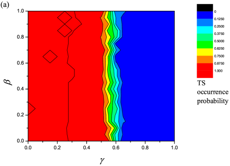
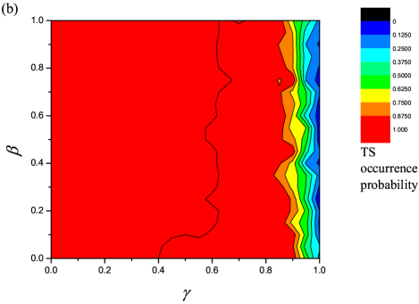
Figure 2: (Color online) The phase diagram in the space of price sensitivity $\gamma$ and market impact $\beta$ for (a) $c_{\mathrm{o}}=100$, and (b) $c_{\mathrm{o}}=925$. Other parameters are $m=2$, $s=2$, $K=3$, $N=1000$ (20 samples).

Figure 3: The time dependence of price for a typical sample with $m=2$, $s=2$, $K=3$, $N=1000$, $c_{\mathrm{o}}=100$ for (a) the trendsetters’ phase at $(\gamma,\beta)=(0.2,0.2)$, (b) the bouncing phase at $(\gamma,\beta)=(0.7,0.2)$.

Figure 4: The virtual wealth of the F, T and B strategies in (a) the TS attractor at $(\gamma,\beta)=(0.2,0.2)$, (b) the BO attractor at $(\gamma,\beta)=(0.7,0.2)$. Parameters: $m=2$, $s=2$, $K=3$, $N=1000$, $c_{\mathrm{o}}=100$.

In another set of experiments, we first prepare the TS attractor in the TS phase, and then inject virtual cash to the B strategy so that the BO attractor is favored. We observe that for all values of $\gamma$, stable BO attractors can be formed when the amount of injected virtual cash is sufficiently large. In the converse experiment, we inject virtual cash to the F strategy in the BO attractor in the BO phase. When $c_{\mathrm{o}}$ is high so that the BO phase is narrow, stable TS attractors are formed at all values of $\gamma$ when the level of injected virtual cash is sufficiently high. However, when $c_{\mathrm{o}}$ is low and the BO phase is broad, we found that at high values of $\gamma$, stable TS attractors cannot be formed no matter how much virtual cash is injected. This indicates that the conditions for forming the TS attractor are probably more restrictive than the BO attractor, and the existence phase of the TS attractor may be studied using approaches to generic transitions. However, this transition is not relevant to the dynamical transitions starting from the unbiased initial conditions discussed in this paper.

III.1 The Bouncing Phase

In the bouncing phase, the dominant strategy is either T or B. In the example shown in Fig. 3(b), the dominant strategy is B. Its dynamics is one large upward jump in price, followed by one or several steps of zero change, and a downward jump in several small steps or one large step. It reflects the desire of the agents who buy stocks to take advantage of a low price, but the price trend is prevented from rising further due to the prevailing pessimistic atmosphere of the market.

The virtual wealth of the strategies are shown in Fig. 4(b). Since the B strategy gains profit from buying immediately before the large upward jump and selling afterwards, it becomes the dominant strategy. The T strategy also gains profit from selling immediately before the downward jumps and buying at a lower price. Hence its virtual wealth also increases with time, but at a rate slower than that of the B strategy. On the other hand, since the F strategy cannot gain wealth in a price series with frequent trend reversals, it becomes a losing strategy.

Besides the up-bouncing example shown in Fig. 3(b), down-bouncing dynamics dominated by the T strategy can also be observed, depending on the initial conditions. Using the gauge symmetry of the game, their mechanism can be explained similarly.

III.2 The Trendsetters’ Phase

This is the phase that gives rise to bubbles and crashes in the cycles of stock prices Giardina03 ; Yeung08 . As shown in Fig. 3(a), the price series consists of alternating long rising and falling trends. As shown in Fig. 4(a), the virtual wealth of the F strategy rises continuously due to its trendy decisions, with minor setbacks when the price trend reverses. On the other hand, the T and B strategies oscillate about their average at the frequency of the price oscillations. Since the T strategy mainly takes a long position, its virtual wealth is higher than that of the B strategy during the upper half of the price cycle. Similarly, the B strategy has a higher virtual wealth during the lower half of the price cycle. The T strategy gains wealth by selling at the peak and buying back at a lower price the next step, and the B strategy gains wealth by buying at the price minimum and selling at a higher price at the next step. Hence their average also has a slowly rising trend.

In the absence of market makers, the steady state is dominated by dry quotations. Hence the cash of different agents becomes stationary when the system equilibrates. For $s=2$, there are six types of agents. Those holding two F strategies are denoted as FF agents, and the other five types are FT, FB, TT, TB and BB agents. In the steady state, agents can be roughly categorized as the active groups (including FF, FT and FB agents) and the inactive group (including TT, TB and BB agents). The active group usually has a relatively large amount of cash, so that the price movement is mostly due to their participation in the quoting activities. The inactive agents usually have little cash, or have already reached the position bounds $(|k_{i}|=K)$, so that their quotations would usually be terminated by the Cash Rule or the position bounds. Due to the unavailability of participation of the inactive group, real transactions cannot materialize as the active agents cannot find matching dealers. Thus in this phase, the price movement is solely caused by dry quoting.

The TS attractor is generally divided into four stages as shown in Fig. 5. In stage 1, all active agents place buying quotes and thus the price is boosted up with the steepest slope. Stage 2 starts when the price has reached a level higher than the cash level of some of the active agents, whose quoting actions are terminated by the Cash Rule, leading to a decrease in the rate of price evolvement. Stage 2 ends when the price is higher than the cash level of the most liquid active agents. A quiet step (i.e. a time step with zero price change) follows as no one quotes. Since the price change is zero, a random signal is generated as the signal input for the next step. If $\uparrow$ is generated, another quiet step follows, until a $\downarrow$ signal is randomly generated, triggering a falling trend. Stages 3 and 4 are duplicates of stages 1 and 2 under the gauge transformation.

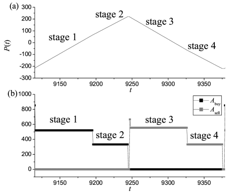
Figure 5: A typical trendsetters’ attractor showing (a) the price evolvement, (b) the evolvements of the total buying and selling quotations. The parameters are $(\gamma,\beta)=(0.2,0.2)$, $m=2$, $s=2$, $K=3$, $N=1000$, $c_{\mathrm{o}}=100$.

In Fig. 5, note that the transition from stage 1 to 2 (or from stage 3 to 4) is not apparent in the price series. This is because TS attractors exist at low $\gamma$, where the price change is weakly sensitive to the excess demand $A(t)$.

In the following sections, we will analyze the behavior of the TS attractor, leading eventually to an estimation of the phase transition point.

IV The Transient Period

In contrast to the trendsetter attractor in Yeung08 , the TS attractor in the absence of market makers is dominated by dry quotations. This implies that the amount of cash held by each agent becomes stationary at the steady state. As will be confirmed in the next section, the period of the price cycles depends on the cash level of the most liquid agent. Hence, the steady state behavior of the price cycles directly depends no how the transient dynamics redistributes the cash into the hands of the different types of agents. This heavy dependence on the transient dynamics is the characteristics of the Wealth Game without market makers.

A typical price series is shown in Fig. 6 when the initial cash $c_{\mathrm{o}}$ is sufficiently large that we are not very close to the phase boundary. At the beginning of the transient stage, a significant redistribution of cash starts to take place in the first half of the quasi-period of the price series. We refer to this as the separation stage. Following the separation stage, the cash levels are roughly flat with occasional jumps, whose magnitudes are progressively smaller. We call this the quasi-stable stage. Eventually, the cash levels become stable at the steady state.

Figure 6: (Color online) The cash evolvements of different agents and the price series in type I TS attractor for (a) the asymptotic time series, (b) the transient, which is further divided into the quasi-stable stage and the separation stage, and (c) the separation stage. The parameters are $(\gamma,\beta)=(0.2,0.8)$, $m=2$, $s=2$, $K=3$, $N=1000$, $c_{\mathrm{o}}=100$, initial conditions ($\downarrow\downarrow$, $\mathrm{B}>\mathrm{F}>\mathrm{T}$).

At the first few steps of the separation stage, the price rises from zero. Some real transactions take place, but since the price is close to zero, the cash levels of the agents do not change much and are roughly equal to $c_{\mathrm{o}}$. After several steps, the major sellers (the BB agents) have reached the minimum position of $-K$. Dry quoting happens again and again, until the price is just higher than $c_{\mathrm{o}}$, at where the agents think the stock is too expensive. The price stops rising and when a downward signal appears, all agents make selling quotations. In the next step, the signal $\downarrow\downarrow$ first appears after the quiet period. Both buying and selling quotations are made by the agents. This is the time when there is a significant redistribution of cash among the agents.

Subsequent to this event, there is a rising or falling price trend depending on the excess demand at the event. For attractors obtained from the initial condition used in Fig. 6, which will be classified as type I attractor, the price follows a rising trend, hits a peak when it goes above the cash level of the most liquid agents. No transactions can be fulfilled as the major sellers (BB) have reached the minimum position already, and the price goes on a falling trend. For other initial conditions, the price follows a falling trend directly after the event. In all cases, such price movements are not accompanied by any real transactions, as the price is higher than the cash levels of the buying group. Hence, no cash redistribution takes place for many time steps.

For type I attractors, the second significant cash redistribution takes place when the price falls below the cash level of the second most liquid group of agents.

In the quasi-stable stage, real transactions can only materialize when the price is close to zero, allowing the inactive agents to participate with their low cash levels. When this happens, the cash levels of the agents fluctuate little bit. These fluctuations are so minor that we can neglect their effects on the final stable cash levels.

Hence we can focus on the cash evolvements in the separation stage to calculate the approximate stable cash levels and hence the amplitude of the price cycles. For the initial condition in Fig. 6, this is done with reference to Tables 3 and 4 at the first and second significant cash redistributions respectively. At the first event, the order of priority of the strategies is T $>$ F $>$ B, leading to the adoption of the strategies in the third column of Table 3. In response to the signal $\downarrow\downarrow$, the outputs of these strategies are given in the fourth column. Taking into account the positions listed in the fifth column, the final decisions of the agents are given in the sixth column. Summing up the buying and selling quotations weighted by the fractions in the second column, we obtain $A_{\mathrm{buy}}=5N/9$ and $A_{\mathrm{sell}}=3N/9$. Thus, the FF and FB agents are the minority and sell one whole unit of stock at the price $P\approx c_{\mathrm{o}}$. Agents in the buying group have bought $3/5$ unit of stocks, and have lost cash $\approx 3c_{\mathrm{o}}/5$.

Table 3: The outputs, positions, decisions and final cash (roughly in multiples of $c_{\mathrm{o}}$) of the agents at the first significant cash redistribution event of a type I TS attractor.

Agents	Fraction	Strategy	Output	Position	Decision	Final cash
FF	$1/9$	F	sell	$\geq-K+1$	sell	2
FT	$2/9$	T	buy	$\leq K-1$	buy	$2/5$
FB	$2/9$	F	sell	$\geq-K+1$	sell	2
TT	$1/9$	T	buy	$\leq K-1$	buy	$2/5$
TB	$2/9$	T	buy	$\leq K-1$	buy	$2/5$
BB	$1/9$	B	sell	$=-K$	hold	1

Table 4: The outputs, positions, decisions and final cash (roughly in multiples of $c_{\mathrm{o}}$) of the agents at the second significant cash redistribution event of a type I TS attractor.

Agents	Fraction	Strategy	Output	Position	Decision	Final cash
FF	$1/9$	F	sell	$\geq-K+1$	sell	$56/25$
FT	$2/9$	F	sell	$\geq-K+1$	sell	$16/25$
FB	$2/9$	F	sell	$\geq-K+1$	sell	$56/25$
TT	$1/9$	T	buy	$\leq K-1$	buy	0
TB	$2/9$	T	buy	$\leq K-1$	buy	0
BB	$1/9$	B	sell	$=-K$	hold	1

At the second event, the price has fallen to just below the cash level of the second most liquid group of agents (FF, TT and TB), which is roughly $2c_{\mathrm{o}}/5$. At this point, the price has fallen to a value such that the order of priority of the strategies becomes F $>$ T $>$ B. Consequently, as shown in Table 4, the FT agents have changed to be in the selling group. We obtain $A_{\mathrm{buy}}=3N/9$ and $A_{\mathrm{sell}}=5N/9$. Hence, agents in the selling group sell $3/5$ unit of stocks at the price $P\approx 2c_{\mathrm{o}}/5$, and so gain cash of the amount $6c_{\mathrm{o}}/25$. The buying agents have their cash reduced by $2c_{\mathrm{o}}/5$.

As mentioned earlier, the maximum price $P_{\mathrm{max}}$ is reached when the price has just exceeded the cash level of the most liquid agents. Therefore, $P_{\mathrm{max}}\approx 56c_{\mathrm{o}}/25$ for type I attractors.

Considering the dynamics starting from all the 24 initial conditions, we classify the TS attractors into three types as shown in Table 5. Their maximum price and the distribution of the final cash are described in Appendix. Although the amplitudes of the price cycles of the three types of attractors are different, their dynamics are qualitatively the same.

Table 5: The three types of TS attractors at $(\gamma,\beta)=(0.2,0.8)$, $m=2$, $s=2$, $K=3$, $N=1000$, $c_{\mathrm{o}}=100$. In the initial conditions, $*$ represents $\uparrow$ or $\downarrow$. Only the 12 initial conditions that give rise to an initial rising trend during the separation stage are included in the third column. The other 12 initial conditions, related to those in the fourth column by gauge transformation $\uparrow\leftrightarrow\downarrow$ and T$\leftrightarrow$B, belong to the same corresponding type of attractor.

Attractor	Most liquid agents	Initial condition	$P_{\mathrm{max}}$
Type I	FF and FB	($*$$*$, T $>$ F $>$ B)	$56c_{\mathrm{o}}/25$
Type II	FT	($*$$\downarrow$, T $>$ B $>$ F)	2$c_{\mathrm{o}}$
Type III	FB	($*$$\uparrow$, T $>$ B $>$ F)	$8c_{\mathrm{o}}/5$
	FF and FT and FB	($*$$\uparrow$, F $>$ B $>$ T) ($*$$\uparrow$, F $>$ T $>$ B)

We have also studied the dynamics of the TS attractors at other values of $K$ and $(\gamma,\beta)$, but whose locations are not close to the boundary of the TS phase. We found TS attractors with approximately the same amplitudes of $56c_{\mathrm{o}}/25$, 2$c_{\mathrm{o}}$, $8c_{\mathrm{o}}/5$, but we also found attractors with other amplitudes such as $14c_{\mathrm{o}}/5$ and $72c_{\mathrm{o}}/35$. An exhaustive search of all possible amplitudes is beyond the scope of our study. Since they have qualitatively similar behaviors, we will continue our analysis using only the three types of attractors we have described.

V Periods of the Price Cycles

After obtaining an estimate of the amplitudes of the price cycles in the previous section, we can derive the periods of the price cycles if we also know about the price change per time step. This information is also available from Table 4 for type I attractor.

Consider the falling trend from the peak price of $P_{\mathrm{max}}\approx 56c_{\mathrm{o}}/25$ to the valley $P\approx-56c_{\mathrm{o}}/25$. From Tables 3 and 4, we find that $A\mathrm{{}_{sell}}=3N/9$ from $P=56c_{\mathrm{o}}/25$ to $P=16c_{\mathrm{o}}/25$, and $A\mathrm{{}_{sell}}=5N/9$ from $P=16c_{\mathrm{o}}/25$ to $P=-56c_{\mathrm{o}}/25$. Hence, the period of the price cycles is given by

$$\frac{T_{\mathrm{I}}}{2} = \left(\frac{3N}{9}\right)^{-\gamma}\left(\frac{56}{25}c_{\mathrm{o}}-\frac{16}{25}c_{\mathrm{o}}\right)$$ (18)

$$+\left(\frac{5N}{9}\right)^{-\gamma}\left(\frac{16}{25}c_{\mathrm{o}}+\frac{56}{25}c_{\mathrm{o}}\right).$$

This reveals the dependence of the period on $c_{\mathrm{o}}$ and $\gamma$

$$T_{\mathrm{I}}=\left(\frac{16c_{\mathrm{o}}}{25N^{\gamma}}\right)\left[5\left(3^{\gamma}\right)+9\left(\frac{9}{5}\right)^{\gamma}\right].$$ (19)

The periods of types II and III attractors are derived in Appendix. To compare with simulation results, we calculate the harmonic mean of the periods averaged over the initial conditions. From Table 5, the probabilities of occurrence are $1/3$, $1/6$ and $1/2$ for types I, II and III attractors respectively. Hence the average period of TS attractors is

$$T_{\mathrm{av}}=\left(\frac{1}{3}T_{\mathrm{I}}^{-1}+\frac{1}{6}T_{\mathrm{II}}^{-1}+\frac{1}{2}T_{\mathrm{III}}^{-1}\right)^{-1}.$$ (20)

Substituting Eqs. (19), (23) and (24), we obtain

$$T_{\mathrm{av}} = \frac{16c_{\mathrm{o}}}{N^{\gamma}}\times$$

$$\left\{\frac{25}{3\left[5\left(3^{\gamma}\right)+9\left(9/5\right)^{\gamma}\right]}+\frac{1}{3\left(3^{\gamma}\right)}+\frac{5}{4}\left(\frac{5}{9}\right)^{\gamma}\right\}^{-1}.$$

So far we have derived this expression for a particular value of $\gamma$ ($=0.2$). Observing that the attractor structures in a broad range of $\gamma$ are qualitatively similar, we extrapolate this result to general values of $\gamma$. Interpolating the expression by an exponential function of $\gamma$ between $\gamma=0$ and $\gamma=1$, we have

$$\mathrm{ln}T_{\mathrm{av}}\approx B-m\gamma,$$ (22)

where $B=\mathrm{ln}\left(448c_{\mathrm{o}}/61\right)$ and $m=\mathrm{ln}\left(3514N/7137\right)$.

Figure 7 shows the average TS period for $c_{\mathrm{o}}=100$ obtained from simulations. It shows that the period is an exponential function of $\gamma$. $B$ and $m$ in the figure are determined experimentally to be 6.71 and 6.13 respectively. This compares favorably with the theoretical prediction of Eq. (22) which yields $B=6.60$ and $m=6.20$.

Figure 7: (Color online) The dependence of the TS period on $(\gamma,\beta)$ averaged over 10 samples. The line is the prediction of Eq. 22. The parameters are $m=2$, $s=2$, $K=3$, $N=1000$, $c_{\mathrm{o}}=100$.

VI The Phase Boundary

To search for the existence condition of the TS phase, we plot the period of the TS attractors as a function of $\gamma$ for various $c_{\mathrm{o}}$ in Fig. 8. Remarkably, the TS attractors disappear when the period falls below an apparently universal value, suggesting that there is a lower bound of the TS period around $4K+5$.

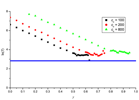
Figure 8: (Color online) The dependence of the TS period on $\gamma$ averaged over the 12 possible attractors for various $c_{\mathrm{o}}$ down to the boundary of the TS phase. The line corresponds to the bound of $4K+5$. The parameters are $s=2$, $K=3$, $\beta=0.5$, $N=1000$.

This possibility is further supported by the numerical experiment described in Fig. 9. We start the Wealth Game with an initial condition biased towards the F strategy, but at a very high value of $\gamma$ deep in the BO phase. This favors the TS attractor in the transient stage, which is expected to be destabilized at the steady state. We observe that the virtual wealth of the F strategy decreases from one period to another and is accompanied by periods of the TS attractor shorter than $4K+5$. Meanwhile, the virtual wealth of the B (or T) strategy keeps on increasing period after period. Eventually, the F strategy is outperformed by the B strategy and the TS attractor disappears.

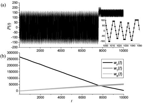
Figure 9: The transient existence of the TS attractor at $(\gamma,\beta)=(0.65,0.5)$ starting with the following virtual cash of the strategies: $c_{\mathrm{F}}=2000N^{\gamma},c_{\mathrm{T}}=c_{\mathrm{B}}=0$, for (a) the price series, where the inset shows the magnified plot of the TS regime and (b) the virtual wealth series. Other parameters are: $s=2$, $K=3$, $N=1000$,$c_{\mathrm{o}}=100$.

Let us analyze the attractors with the shortest possible TS period. As shown in Fig. 10 for a TS attractor, the F strategy starts from the minimum position $-K$ at the beginning of stages 1 and 2, and takes buying actions in response to the signal $\uparrow\uparrow$ for $2K$ steps. This continues until it reaches the maximum position $K$. A quiet period follows. The signal at the first step of the quiet period is $\uparrow\uparrow$, but the signals in the following steps are random. If the signal is $\uparrow$, the quiet period continues, but if the signal is $\downarrow$, all strategies respond to $\uparrow\downarrow$ by selling, and the dynamics enters stage 3. Hence the average length of the quiet period is $1+\sum_{n=0}^{\infty}n/2^{n+1}=2$.

Figure 10: The time series of (a) the price and (b) the virtual wealth of the F strategy in a half-period of the TS attractor at $(\gamma,\beta)=(0.55,0.8)$, $s=2$, $K=3$, $N=1000$, $c_{\mathrm{o}}=100$. Note that in general, the F strategy requires $2K$ steps to regain the virtual wealth at the previous quiet period when $\beta\leq 0.5$, and $2K+1$ steps when $\beta>0.5$.

When the falling price trend of stage 3 starts, the F strategy makes the right move of selling, but its position remains positive due to the rising trend in stages 1 and 2. It takes the strategy $K$ steps to change its position to $0$. As shown in Fig. 10, it is losing virtual wealth during this period of time. It takes another $K$ steps to change its position from zero to minimum, and the strategy is regaining virtual wealth during this period. For these $2K$ steps, its virtual wealth gain and loss are roughly balanced. This completes the adjustment stage of the F strategy. If the falling trend is longer than $2K$ steps, then the strategy can start to gain virtual wealth using its trend-following outputs and stabilize the TS attractor.

To make a more quantitative estimate, we consider the case $\gamma=0$, in which the price change at each step is $A^{0}=1$, independent of the volume of buying and selling quotations. By tracing the virtual wealth change of the F strategy during a price cycle of length $4K+4$ (with an average length of 2 during the quiet periods at the peaks and valleys), the virtual wealth gain of the F strategy is calculated to be $2K(1-2\beta)$, whereas those of the T and B strategies are 1. When the period of the price cycle lengthens, the virtual wealth gain of the F strategy increases by $K$ for every extension of the period by one step. If we consider the mid-position of the phase diagram with $\beta=1/2$, then for price cycles of period $4K+5$, the F strategy outperforms the T and B strategies by $2K(1-2\beta)+K-1=K-1$. Hence for $K>1$, it is reasonable to estimate the phase boundary by the condition that the period of the price cycle becomes $4K+5\equiv T_{\mathrm{c}}$.

We are now ready to calculate the critical value $\gamma_{\mathrm{c}}$ of the TS attractor at the phase boundary. However, we observe in Fig. 2 that the transition to the BO phase occurs within a narrow but finite range of $\gamma$, instead of having an abrupt change. This is due to the dependence on the initial conditions, as classified according to the three types of attractors. By equating $T_{\mathrm{c}}$ to the periods in Eqs. (19), (23) and (24), we find that $\gamma_{\mathrm{c}}$ takes the values of 0.65, 0.66 and 0.57 for types I, II and III attractors respectively. The phase lines for types II and III attractors are located in the phase diagrams in Fig. 11, and the matching with the simulation results is quite well.

Figure 11: (Color online) Comparison of the theoretical prediction of $\gamma_{\mathrm{c}}$ with the simulation results for (a) $c_{\mathrm{o}}=100$ and (b) $c_{\mathrm{o}}=925$. Other parameters are $s=2$, $K=3$, $N=1000$ (20 samples).

VII Dependence on Population Composition

So far, we have considered the case of unbiased assignment of strategies, that is , $f_{\mathrm{F}}:f_{\mathrm{T}}:f_{\mathrm{B}}=1:1:1$, where $f_{\mathrm{\sigma}}$ is the ratio of the probabilities of assigning strategies $\mathrm{\sigma}$ to an agent. It is interesting to consider how the market dynamics changes when we vary the ratio of strategies to $f_{\mathrm{F}}:f_{\mathrm{T}}:f_{\mathrm{B}}=f:1:1$, where $f$ is referred to as the trendsetter (TS) factor. Figure 12 shows the phase diagram in the space of $f$ and $\gamma$. The TS phase exists for sufficiently large $f$ and sufficiently small $\gamma$. This suggests that in order to trigger the TS price trends, the market should be dominated by enough trendsetting strategies. In other words, a market is trendy only when there are enough trend-believing agents. In contrast, if the game is full of T and B strategies, it becomes a market with fundamentalists as the majority, and price trends cannot be set up easily. Such a picture shows qualitative consistency with the results obtained in Giardina03 , where a polarization parameter determines the statistical weight of trend-following strategies, and the periodic phase exists at high polarization.

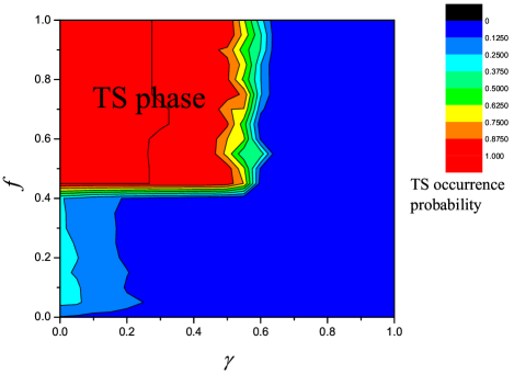
Figure 12: (Color online) The phase diagram in the space of the F strategy factor $f$ and price sensitivity $\gamma$. Other parameters are $s=2$, $K=3$, $N=1000$, $c_{\mathrm{o}}=100$, $\beta=0.5$ (20 samples).

The vertical segment of the phase boundary in Fig. 12 shows little dependence on $f$, indicating that our analysis at $f=1$ is a good approximation. To analyze the horizontal segment, we consider the typical attractor profile below and above the phase boundary in Fig. 13. Note that at the transient stage, the price series in both cases appear as TS. The difference lies in the behavior on approaching the steady state. When $f$ is small, the F-group agents (FF, FT and FB) are the minority. In the absence of market makers, the need to balance the buying and selling volumes has significant consequences in determining the types of agents whose positions are saturated (that is, reach $\pm K$). Hence, we show the evolvement of the agents’ positions in Fig. 14 during the separation stage for two typical cases. In these cases the position of the F-group agents saturate at $K$; the cases of $-K$ have the same behavior after gauge transformation.

Figure 13: The price series of an attractor before and after undergoing the phase transition at (a) $f=0.4$ (b) $f=0.5$. The middle plot and the top table are the magnified graph of the price series and the positions of different agents at stable states. Other parameters are $m=2$, $s=2$, $K=3$, $N=1000$, $c_{\mathrm{o}}=100$, $(\gamma,\beta)=(0.2,0.8)$, initial condition $(\uparrow\uparrow,\mathrm{T}>\mathrm{F}>\mathrm{B})$.

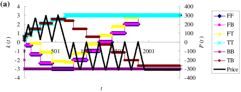
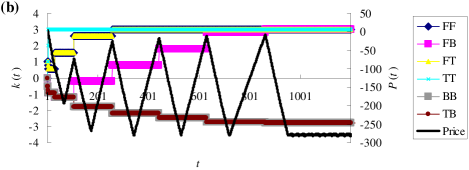
Figure 14: (Color online) Evolvement of the agents’ positions for initial condition (a) ($\uparrow\uparrow,\mathrm{T}>\mathrm{F}>\mathrm{B}$), (b) ($\downarrow\uparrow,\mathrm{B}>\mathrm{F}>\mathrm{T}$). The price series is also shown for reference. Parameters: $s=2$, $K=3$, $N=1000$, $c_{\mathrm{o}}=100$, $(\gamma,\beta)=(0.2,0.8)$, $f=0.4$.

The outcome of the separation stage is that the TT and F-group agents take up positive positions at the steady state, and the BB and TB agents have negative positions. Note that at the steady state, the only active sellers with unsaturated positions are the TB agents in Fig. 14(a), and the TB and BB agents in Fig. 14(b). More significantly, the F-group agents have saturated positive positions. Once their positions are saturated, their buying quotations disappear. The TS price trend stops, and the steady state enters the bouncing attractor.

This transition mechanism from the TS transient to the BO attractor is further confirmed by the dynamics of agents’ positions when $f$ is increased to enter the TS phase, as shown in Fig. 15. Since $f$ is larger when compared with Fig. 14, the TB and BB agents saturate at position $-K$ before the F-group agents reaches position $K$. The result is exactly the opposite: the selling quotes of the TB and BB agents disappear, and the price continues to rise. More important, the F-group agents remain unsaturated. They emerge as active agents with the freedom to make buying and selling quotes, and the TS attractor is sustainable at the steady state.

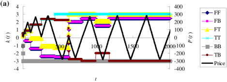
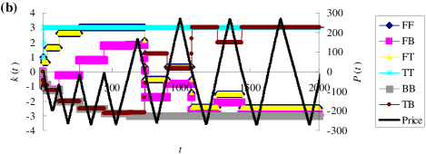
Figure 15: (Color online) Same as Fig. 14, except that $f=0.5$.

This transition mechanism enables us to derive the macroscopic condition for the disappearance of the TS phase, irrespective of the transaction details. The total volume of stocks that can be sold by the BB and TB agents is $V_{\mathrm{s}}=3NK/(2+f)^{2}$. The total volume of stocks that can be bought by the TT and F-group agents is $V_{\mathrm{b}}=NK(f^{2}+4f+1)/(2+f)^{2}$. If $V_{\mathrm{b}}<V_{\mathrm{s}}$, the F-group agents become saturated and remain inactive. Thus we have the BO phase when $f<\sqrt{6}-2\approx 0.449$. This prediction matches well with the simulation result in Fig. 12.

VIII Conclusion

We have considered a simplified Wealth Game in which no market makers are present. Since buying and selling quotations are not balanced, the dynamics becomes complicated. Furthermore, due to the prevalence of dry quotations, the dynamics becomes heavily dependent on the initial conditions. This makes it difficult to analyze the model and understand its underlying mechanism. To circumvent this difficulty, we simplify the input dimension of the strategies to 2 and restrict the strategies to three representative ones, namely, F, T and B. Respectively, they represent the trend-followers/trendsetters, optimistic and pessimistic fundamentalists in the market.

With these simplifications, we observe a dynamical transition from the TS phase to the BO phase when $\gamma$ increases. Despite the simplicity of the model, both phases bear characteristics of real markets. The TS phase produces price trends that resemble bubbles and crashes in real markets. They are observed when the agents have enough cash, and the price movement is not very sensitive to the excess demand. The BO phase produces price trends that are relatively steady, with occasional up-bounces or down-bounces followed by relaxations to fundamental prices. These price trends can also be observed in real markets when investors have very cautious moods about the fundamental values of the stocks. Both phases are dominated by dry quotations, which correspond to quiet moments in real markets with very low trading volumes. In many economic systems, such as the real estates market, dry quotations are prevalent when the price is too high or too low.

We find that the amplitude of the price cycles is determined by the cash level of the most liquid agents. When agents with less cash stop their quotations, the more liquid agents can still boost up or push down the price to higher or lower levels. Prices reach their extreme values when the agents consider it too risky to participate. However, the quantitative relation between the price amplitude and the initial cash is determined by the cash redistribution process during the transient stage. To overcome the complexity of this process, we adopt a semi-empirical approach by analyzing the separation stage for various initial conditions, and extrapolating the predictions to the entire TS phase. Agreement with simulation results shows that this is a good approximation.

Our study also suggests a mechanism for the disappearance of the TS phase. All trend-following strategies need an adaptation period when the price trend reverses. Agents become certain of the advantages of these strategies only when the duration of a price trend is longer than that of the adaptation period. When the price sensitivity increases, the price change per step increases, and the period of the price cycles shortens. When the period becomes comparable to the adaptation period, the TS attractor becomes unsustainable.

We also find that the composition of the population affects the market behavior. The TS phase is present in markets where trend-following strategies are popular. When the trend-following strategies become less popular, we observe a phase transition to the bouncing phase. We find that this transition is due to the fact that the positions of the trend-followers saturate at the maximum (or minimum), and no active agents want to buy (or sell) when they decide to sell (or buy). This allows us to derive a macroscopic condition for the phase transition by balancing the volume of supply and demand of stocks. The prediction agrees with the simulation results well.

It is interesting to compare our model with the Wealth Game with the market makers present Yeung08 . In both cases, the TS phase exists due to the presence of trend-followers. However, when market makers are present, the price trend is driven by real transactions and has a slightly different dynamics. For example, the so-called fickle agents are those who hold a T and B strategy, and fickle their preference between the two strategies with a delayed response. They push the price further up in a rising trend, and down in a falling trend, thus creating opportunities for the trend-followers to gain wealth. In our model without market makers, the fickle agents do not play an important role. During the separation stage, their cash is reduced to a very low level, as evident in Tables 4, 6 and 7 for types I to III attractors respectively. Hence they only play a minor role in the price dynamics.

While our model is successful in explaining and interpreting a number of market phenomena, it can be further improved to address a broader range of issues. One possible modification to this model is to implement the injection of cash to the market. This may help to relieve the problem of too many dry quotations in the present model, whose agents are restricted by the cash rule. Furthermore, since the present model is a close system with constant average wealth, incorporating cash injection may cause the market to evolve spontaneously towards states which have maximal attraction of capital. In this way, it will also address the issue of the self-organization of markets, which has drawn considerable attention in recent models Giardina03 ; Challet01 ; Yeung08 ; Alfi09a ; Alfi09b .

Appendix A Periods of Types II and III Attractors

In a type II attractor, there is only one significant cash redistribution event during the separation stage. It takes place during a falling trend, and the order of priority of the strategies is F $>$ T $>$ B. Both FB and BB agents have reached their minimum positions. As calculated in Table 6, $A_{\mathrm{buy}}=A_{\mathrm{sell}}=3N/9$, and the maximum final cash is $2c_{\mathrm{o}}$. Hence $P_{\mathrm{max}}\approx 2c_{\mathrm{o}}$.

The period of type II attractor is

$$T_{\mathrm{II}}=\frac{8c_{\mathrm{o}}}{N^{\gamma}}3^{\gamma}.$$ (23)

Table 6: The outputs, positions, decisions and final cash (in multiples of $c_{\mathrm{o}}$) of the agents at the cash redistribution event of a type II attractor.

Agents	Fraction	Strategy	Output	Position	Decision	Final cash
FF	$1/9$	F	sell	$\geq-K+1$	sell	2
FT	$2/9$	F	sell	$\geq-K+1$	sell	2
FB	$2/9$	F	sell	$=-K$	hold	1
TT	$1/9$	T	buy	$\leq K-1$	buy	0
TB	$2/9$	T	buy	$\leq K-1$	buy	0
BB	$1/9$	B	sell	$=-K$	hold	1

In a type III attractor, there is often only one significant cash redistribution event during the separation stage. It takes place during a falling trend, and the order of priority of the strategies is F $>$ T $>$ B. Only the BB agents have reached their minimum positions. As calculated in Table 7, $A_{\mathrm{buy}}=3N/9$ and $A_{\mathrm{sell}}=5N/9$, and the maximum final cash is $8c_{\mathrm{o}}/5$. Hence $P_{\mathrm{max}}\approx 8c_{\mathrm{o}}/5$.

Table 7: The outputs, positions, decisions and final cash (in multiples of $c_{\mathrm{o}}$) of the agents at the cash redistribution event of a type III attractor.

Agents	Fraction	Strategy	Output	Position	Decision	Final cash
FF	$1/9$	F	sell	$\geq-K+1$	sell	$8/5$
FT	$2/9$	F	sell	$\geq-K+1$	sell	$8/5$
FB	$2/9$	F	sell	$\geq-K+1$	sell	$8/5$
TT	$1/9$	T	buy	$\leq K-1$	buy	0
TB	$2/9$	T	buy	$\leq K-1$	buy	0
BB	$1/9$	B	sell	$=-K$	hold	1

Besides the single event described in Table 7, there are also initial conditions which result in TT and TB holding slightly different amount of cash before significant cash redistribution occurs. This gives rise to the occurrence of two events, but the final cash distribution remains the same.

The period of type III attractor is

$$T_{\mathrm{III}}=\frac{32c_{\mathrm{o}}}{5N^{\gamma}}\left(\frac{9}{5}\right)^{\gamma}.$$ (24)

References

- (1) D. Challet and Y.-C. Zhang, Physica A 246, 407 (1997).
- (2) D. Challet, M. Marsili, and Y.-C. Zhang, Minority Games (Oxford University Press, Oxford, UK, 2005).
- (3) R. Savit, R. Manuca, and R. Riolo, Phys. Rev. Lett. 82, 2203 (1999).
- (4) A. Cavagna, J. P. Garrahan, I. Giardina, and D. Sherrington, Phys. Rev. Lett. 83, 4429 (1999).
- (5) R. Jefferies, M. L. Hart, P. M. Hui, and N. F. Johnson, Eur. Phys J. B 20, 493 (2001).
- (6) J. V. Andersen and D. Sornette, Eur. Phys. J. B 31, 141 (2003).
- (7) M. Marsili, Physica A 299, 93 (2001).
- (8) A. De Martino, I. Giardina, and G. Mosetti, J. Phys. A: Math. Gen. 36, 8935 (2003).
- (9) T. Lux and M. Marchesi, Nature 397, 498 (1999).
- (10) A. De Martino, I. Giardina, A. Tedeschi, and M. Marsili, Phys. Rev. E 70, 025104(R) (2004).
- (11) D. Challet, J. Econ. Dyn. Control 32, 85 (2008).
- (12) C. H. Yeung, K. Y. Michael Wong, and Y.-C. Zhang, Phys. Rev. E 77, 026107 (2008)
- (13) Y. Baek, S. H. Lee, and H. Jeong, Phys. Rev. E 82, 026109 (2010).
- (14) I. Giardina and J.-P. Bouchaud, Eur. Phys. J. B 31, 421 (2003).
- (15) D. Challet, M. Marsili, and Y.-C. Zhang, Physica A 276 284 (2000).
- (16) M. Marsili, D. Challet, and R. Zecchina, Physica A 280, 522 (2000).
- (17) D. Challet, M. Marsili, and R. Zecchina, Phys. Rev. Lett. 84, 1824 (2000).
- (18) J. A. F. Heimel and A. C. C. Coolen, Phys. Rev. E 63, 056121 (2001).
- (19) G. Caldarelli, M. Marsili, and Y.-C. Zhang, EPL 40, 479 (1997).
- (20) F. Slanina and Y.-C. Zhang, Physica A 272, 257 (1999).
- (21) J. D. Farmer, Computing in Science and Engineering 1, 26 (1999).
- (22) D. Challet, A. Chessa, M. Marsili, and Y. C. Zhang, Quant. Finance 1, 168 (2001).
- (23) V. Alfi, M. Cristelli, L. Pietronero, and A. Zaccaria, J. Stat. Mech., P03016 (2009).
- (24) V. Alfi, L. Pietronero, and A. Zaccaria, Europhys. Lett. 86, 58003 (2009).