Holographic Anyons in the ABJM Theory Shoichi Kawamoto and Feng-Li Lin

Department of Physics, National Taiwan Normal University,
Taipei, Taiwan 11677

We consider the holographic anyons in the ABJM theory from three different aspects of AdS/CFT correspondence. First, we identify the holographic anyons by using the field equations of supergravity, including the Chern-Simons terms of the probe branes. We find that the composite of D$p$-branes wrapped over $\mathbf{CP}^{3}$ with the worldvolume magnetic fields can be the anyons. Next, we discuss the possible candidates of the dual anyonic operators on the CFT side, and find the agreement of their anyonic phases with the supergravity analysis. Finally, we try to construct the brane profile for the holographic anyons by solving the equations of motion and Killing spinor equations for the embedding profile of the wrapped branes. As a by product, we find a BPS spiky brane for the dual baryons in the ABJM theory.

1 Introduction

Anyons proposed in [1, 2, 3] are the point particles obeying the fractional statistics, and they exist in $2+1$ dimensions because the linking number in $2+1$ dimensions is well-defined. When the positions of two anyons are interchanged, the wavefunction of the system will get a fractional phase. Moreover, these anyonic particles can be described by $U(1)$ Chern-Simons effective field theory [4]. Namely, via the coupling to the Chern-Simons term the electrons are endowed with a fictitious magnetic flux, which will induce Aharonov-Bohm (AB) phase when one is going around another. Since the exchange of two particles is considered as the half-winding, this AB phase is responsible for the fractional statistics. One example of the above construction is the effective field theory of the quasiparticles for the fractional quantum Hall fluids [5]. The generalization to use D-branes/noncommutative Chern-Simons for describing quantum Hall fluids can be seen in [6], and the related holographic construction was done recently in [7].

Since the anyon is usually thought of as a quasiparticle in a strongly coupled system, and cannot be seen in the perturbative approach. It is then interesting to see if one can construct anyons from the holographic dual of some strongly coupled systems so that anyons can be realized as D-brane configurations. Motivated by the relation between anyons and the $(2+1)$-dimensional Chern-Simons theory, it seems that the recently constructed Aharony-Bergman-Jafferis-Maldacena (ABJM) theory [9] is a good starting point for our purpose, since the ABJM theory is given as $\mathcal{N}=6$ superconformal Chern-Simons-matter theory in $2+1$ dimensions and also its gravity dual of type IIA supergravity in $AdS_{4}\times\mathbf{CP}^{3}$ background is known. Naively, the holographic anyon we are seeking for should be quite different from the one in the usual $U(1)$ Chern-Simons effective field theory. The main reason is that the latter is a quasiparticle consisting of electrons and is thus not gauge invariant, and therefore would not be observed in the bulk gravity side into which only the gauge invariant states are mapped. However, as we will see the holographic anyons are indeed not gauge invariant states in the dual field theory, but still can be observed.

We can generalize the case with $U(1)$ Chern-Simons to the non-abelian one by introducing the ’t Hooft disorder operators. They are defined as the large gauge transformation along a given contour, and also known as ’t Hooft loop. If the theory contains no charged matter under the center of the gauge group, the ’t Hooft disorder operator is local, that is, any field in the action cannot detect the presence of the ’t Hooft operator. However, as shown in [15], in the presence of the Chern-Simons term the ’t Hooft operators can detect each other and thus behave like anyons. In the ABJM case, the ’t Hooft operators are attached to the chiral primary operators that are dual to the D0-brane and D4-branes wrapping on a cycle inside $\mathbf{CP}^{3}$, and makes these operators gauge invariant. Therefore, such gauge invariant states are by definition local under large gauge transformation, and cannot be the anyons.

A way out is to consider the wrapped D2 and D6-branes over $\mathbf{CP}^{3}$. There should be fundamental strings stretching between the branes and the boundary due to the charge conservation on the world volume. They are dual to the baryon vertex [10] in the field theory side, and are similar to the wrapped D5-brane in the case of $AdS_{5}\times S^{5}$ [23]-[26]. Moreover, these baryons are not the gauge invariant states due to the fundamental strings stretching to the boundary. They will therefore pick up a fractional phase under the action of ’t Hooft loop. It then implies that we can make anyons in the ABJM theory by considering the bound states of baryons and ’t Hooft disorder operators. Indeed, we find that the holographic anyons are what we call the dressed baryons, namely, the bound state of baryons, chiral primaries and ’t Hooft disorder operators.

With the above consideration in mind, one can directly look for the holographic anyons by studying the supergravity equations of motion with probe brane sources. Indeed, in [11] Hartnoll has used this approach to construct anyonic strings and membranes in various AdS spaces. The supergravity Chern-Simons terms which couple the background fluxes are responsible for the resultant fractional AB phases when winding one probe brane around the other. In the ABJM theory, we can also construct this kind of anyonic D0-brane and F-string pair, as well as the D4-F1 pair. They are holographic anyons, but their anyonic phases are $1/N$ suppressed in the ’t Hooft limit as in [11].

The holographic anyons we will construct are made of baryonic spiky branes and magnetic fluxes introduced on their world-volumes. On these baryonic branes we need to attach either $k$ or $N$ fundamental strings to satisfy the charge conservation condition. Since $k$ and $N$ will be of order $N$ quantities, then the anyonic phases gained by the set of strings are no longer suppressed in the large $N$ limit. Moreover, the magnetic fields on the D-brane worldvolume can be thought of as dissolved D-branes, these holographic anyons are in fact bound states of particle-like branes wrapped on the internal $\mathbf{CP}^{3}$. Obviously, these holographic anyons should be the anyonic dressed baryons discussed above. We find that these anyons have the anyonic phases proportional to either the ’t Hooft coupling or its inverse , which will not be suppressed in the ’t Hooft limit.

More precisely, from the supergravity analysis we find that the anyonic phase arises either from winding the spiky D2 with $k$ fundamental strings around the D0 (including the dissolved ones on higher wrapped branes), or from winding the spiky D6 with $N$ fundamental strings (with the opposite orientation to the spiky D2’s) around the the wrapped D4. Furthermore, we find the agreement of these anyonic phases with the ones from the field theory analysis, where the non-perturbative effect due to ’t Hooft loop is involved.

We also explore these particle-like branes and their bound states from the open string picture by solving the worldvolume’s equations of motion and the Killing spinor equations for supersymmetric embedding of wrapped D-branes. As a by-product, we find the BPS D2 spiky baryonic-branes in the ABJM theory. In terms of the form of the solution these spiky solutions are quite nontrivial. However, our holographic anyons are not BPS states.

We organize the paper as follows. In the next section we will review Hartnoll’s idea [11] on constructing the anyonic branes with new examples in the ABJM theory, and also set up the notations. In the section 3 using field equations of supergravity we show that some wrapped branes with magnetic fluxes can be realized as the holographic anyons in the ABJM theory. We find that the phase is essentially given by strings from D2-baryon going around D0-branes, or D6-baryon around wrapped D4-branes. In the section 4 we discuss the field theory interpretation of the holographic anyons found in the previous section. Moreover, we find that the anyonic phases from field theory analysis agree with the ones found in the supergravity side. In the section 5 we solve the equations of motion and the Killing spinor equations for the wrapped D-branes of holographic anyons. We conclude our paper in the section 6. Some minor details, convention setup and useful formulas are put in two Appendices A and B, and the details of our trial for solving BPS D4 and spiky D6 wrapped branes in Appendix C.

2 Anyonic pair in ABJM

The anyonic branes were first considered by Hartnoll in [11] where he used field equations of supergravity to show that some pair of branes will pick up a fractional AB phase when one brane transverses the other, and thus are anyonic. He considered the examples of F-D strings in $AdS_{5}\times S^{5}$ and membranes in $AdS_{7}\times S^{4}$ based on the nontrivial topology of configuration space in higher dimensions such as $H_{2}(\mathbb{R}^{4}\setminus\mathbb{R})=H_{3}(\mathbb{R}^{6}\setminus\mathbb{R}^{2})=\mathbb{Z}$. Instead of reciting his examples, we consider an anyonic pair of branes in the ABJM theory, and at the same time set up the notations. As we shall see, the anyonic pair is the D0-brane and F1-string based on the nontrivial topology of configuration space $H_{1}(\mathbb{R}^{3}\setminus\mathbb{R})=\mathbb{Z}$ for D0 going around F1 and $H_{2}(\mathbb{R}^{3}\setminus\{0\})=\mathbb{Z}$ for F1 surrounding D0.

We start with the relevant part of the IIA action in the Einstein frame with also the source terms due to the presence of various strings and branes [8]

$$L= - {1\over 4\kappa^{2}_{10}}\int\left(e^{-\Phi}H_{3}\wedge*H_{3}+e^{3\Phi\over 2}F_{2}\wedge*F_{2}+e^{\Phi/2}\tilde{F}_{4}\wedge*\tilde{F}_{4}+B_{2}\wedge F_{4}\wedge F_{4}\right)$$ (2.1)

$$- \mu_{0}\int_{D0}C_{1}-T_{F1}\int_{F1}B_{2}-\mu_{2}\int_{D2}\left(C_{3}+C_{1}\wedge{\tilde{B}}_{2}\right)$$

$$- \mu_{4}\int_{D4}\left(C_{5}+C_{3}\wedge{\tilde{B}}_{2}+{1\over 2}C_{1}\wedge{\tilde{B}}_{2}\wedge{\tilde{B}}_{2}\right)$$

$$- \mu_{6}\int_{D6}\left(C_{7}+C_{5}\wedge{\tilde{B}}_{2}+{1\over 2}C_{3}\wedge{\tilde{B}}_{2}\wedge{\tilde{B}}_{2}+{1\over 6}C_{1}\wedge{\tilde{B}}_{2}\wedge{\tilde{B}}_{2}\wedge{\tilde{B}}_{2}\right)\;.$$

where $\tilde{F}_{4}=F_{4}-C_{1}\wedge H_{3}$, $2\kappa^{2}_{10}=(2\pi)^{7}\ell_{s}^{8}$, $T_{F1}=\mu_{1}$, and $\mu^{2}_{p}={\pi\over\kappa^{2}_{10}}(2\pi\ell_{s})^{2(3-p)}$ so that $2\kappa^{2}_{10}\mu_{p}=(2\pi\ell_{s})^{7-p}$, and the integrations $\int_{Dp}$ or $\int_{F1}$ are integrated over the worldvolume of the corresponding source branes. Moreover, ${\tilde{B}}_{2}=B_{2}+2\pi\ell_{s}^{2}dA_{1}$ with $dA_{1}$ the magnetic fluxes being turned on in the D-brane worldvolume. Hereafter, we will set $\ell_{s}=1$ for simplicity.

From the action, we can derive the field equations for $C_{3}$, $B_{2}$ and $C_{1}$ as follows:

$$d*(e^{\Phi/2}\tilde{F}_{4})=-H_{3}\wedge F_{4}-2\kappa^{2}_{10}\mu_{2}\delta^{7}(x_{D2})-2\kappa^{2}_{10}\mu_{4}{\tilde{B}}_{2}\delta^{5}(x_{D4})-\kappa^{2}_{10}\mu_{6}{\tilde{B}}_{2}\wedge{\tilde{B}}_{2}\delta^{3}(x_{D6})\;,$$ (2.2)

$$d*(e^{-\Phi}H_{3})+F_{2}\wedge*(e^{\Phi/2}\tilde{F}_{4})+C_{1}\wedge H_{3}\wedge F_{4}-{1\over 2}F_{4}\wedge F_{4}-2\kappa^{2}_{10}T_{F1}\delta^{8}(x_{F1})$$

$$-2\kappa^{2}_{10}\mu_{4}C_{3}\delta^{5}(x_{D4})-2\kappa^{2}_{10}\mu_{6}(C_{5}+C_{3}\wedge{\tilde{B}}_{2})\delta^{3}(x_{D6})=0\;,$$ (2.3)

and

$$d*(e^{3\Phi/2}F_{2})-H_{3}\wedge*(e^{\Phi/2}\tilde{F}_{4})+2\kappa^{2}_{10}\mu_{0}\delta^{9}(x_{D0})+2\kappa^{2}_{10}\mu_{2}{\tilde{B}}_{2}\delta^{7}(x_{D2})$$

$$+\kappa^{2}_{10}\mu_{4}{\tilde{B}}_{2}\wedge{\tilde{B}}_{2}\delta^{5}(x_{D4})+{1\over 3}\kappa^{2}_{10}\mu_{6}{\tilde{B}}_{2}\wedge{\tilde{B}}_{2}\wedge{\tilde{B}}_{2}\delta^{3}(x_{D6})=0\;,$$ (2.4)

where $\delta^{9-p}(x_{p})$ is the Poincaré dual $(9-p)$-form to the worldvolume of Dp-brane as defined by $\int_{Dp}C_{p+1}=\int C_{p+1}\wedge\delta^{9-p}(x_{p})$ with the second integral over the whole spacetime. Note that we arrive (2.3) by using (2.2) so that the terms like $C_{1}\wedge\tilde{B}_{2}\delta^{5}(x_{D4})$ and $C_{1}\wedge\tilde{B}_{2}\wedge\tilde{B}_{2}\delta^{3}(x_{D6})$ are canceled out.

We will consider the ABJM background [9] as follows (see Appendix B for more detailed expressions.)

$$ds_{E}^{2}=e^{-\Phi^{(0)}/2}{R^{3}\over k}({1\over 4}ds^{2}_{AdS_{4}}+ds^{2}_{CP^{3}})$$ (2.5)

and

$$e^{2\Phi^{(0)}}={R^{3}\over k^{3}}\;,\qquad F_{4}^{(0)}=dC_{3}^{(0)}={3\over 8}R^{3}\hat{\epsilon}_{4}\,\qquad F_{2}^{(0)}=dC_{1}^{(0)}={k}J$$ (2.6)

where the superscript $(0)$ denotes that they are the background values, $\hat{\epsilon}_{4}$ is the volume element of unit $AdS_{4}$, and $J$ is proportional to the Kähler form of $\mathbf{CP}^{3}$.

From this, we have

$$*(e^{\Phi^{(0)}/2}F_{4}^{(0)})={6\over k}R^{6}\hat{\epsilon}_{6}$$ (2.7)

where $\hat{\epsilon}_{6}$ is the volume element of unit $\mathbf{CP}^{3}$. Moreover, the volume of unit $\mathbf{CP}^{3}$ is the same as unit $6$-sphere’s, i.e., $vol_{\mathbf{CP}^{3}}={\pi^{3}\over 6}$.

Now, let us consider adding a source D0 particle in the ABJM background and then transversing a probe F1 string around it. From (2.4), at the linear order in the fluctuations we have

$$H_{3}\wedge\hat{\epsilon}_{6}={k\over 6R^{6}}\left((2\pi)^{7}\delta^{9}(x_{D0})+e^{3\Phi^{(0)}/2}d*F_{2}+\frac{3}{2}d*(e^{3\Phi^{(0)}/2}\Phi F_{2}^{(0)})\right)$$ (2.8)

where $H_{3}$, $F_{2}$ and $\Phi$ are linear perturbations on top of the ABJM background due to the presence of the D0 source.

Then, there is an asymptotic anyonic phase picked up by the partition function of the fundamental string probe after transversing around the D0 as follows

$$\Delta\phi_{F1D0} = -T_{F1}\int_{\partial\Sigma}B_{2}$$ (2.9)

$$= -T_{F1}{1\over vol_{\mathbf{CP}^{3}}}\int_{\partial\Sigma\times\mathbf{CP}^{3}}B_{2}\wedge\hat{\epsilon}_{6}\qquad\qquad\qquad[\mbox{as}\;\;r_{min}\longrightarrow\infty]$$

$$= -T_{F1}{1\over vol_{\mathbf{CP}^{3}}}\int_{\Sigma\times\mathbf{CP}^{3}}H_{3}\wedge\hat{\epsilon}_{6}$$

$$= -T_{F1}{1\over vol_{\mathbf{CP}^{3}}}{k\over 6R^{6}}\int_{\Sigma\times\mathbf{CP}^{3}}\left((2\pi)^{7}\delta^{9}(x_{D0})+e^{3\Phi/2}d*F_{2}+\frac{3}{2}d*(e^{3\Phi^{(0)}/2}\Phi F_{2}^{(0)})\right)$$

$$= -{2\pi\over N}-{2\pi\over N}{1\over(2\pi)^{7}}e^{3\Phi^{(0)}/2}\int_{\partial\Sigma\times\mathbf{CP}^{3}}*F_{2}.$$

where $\partial\Sigma$ is the worldvolume swept by the probe fundamental string. In the above the second step is justified by assuming the minimal distance $r_{min}$ between F1 and D0 are large enough so that $B_{2}$ sourced by D0 is independent of the $\mathbf{CP}^{3}$ coordinates, i.e., suppressing the higher harmonics. Moreover, in the third step we have used the Stokes’ theorem, for its validity we need to close up the swept surface $\partial\Sigma$ with the D0 being enclosed. However, if the fluctuations $F_{2}$ and $H_{3}$ are suppressed in the large $r$ limit, we can just fix the IR end point of F1, and move the UV one to sweep out a cone-like surface $\partial\Sigma$ in the bulk as shown in Fig. 1. Indeed, as shown in the Appendix A, both $F_{2}$ and $H_{3}$ are massive and will be suppressed in the large $r$ limit. Moreover, this also implies that the dynamical part of the above phase, i.e., $\int*F_{2}$, can be neglected if the separation between the source and probe is large enough. Finally, from the fourth line to the fifth line, we have used the fact that since $F_{2}^{(0)}$ is the 2-form inside the $\mathbf{CP}^{3}$, $d*(\Phi F_{2}^{(0)})$ is a 9-form schematically written as $\hat{\epsilon}_{4}\wedge f_{5}$ where $f_{5}$ is a 5-form inside the $\mathbf{CP}^{3}$, and thus it trivially vanishes in the integral.

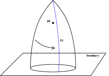
Figure 1: The world sheet of fundamental string surrounding D0-brane.

Similarly, we consider putting a source F1 string in the ABJM background and take a probe D0 particle to transverse it. From (2.3), at linear order in the fluctuations we have

$$F_{2}\wedge\hat{\epsilon}_{6}= {k\over 6R^{6}}\left((2\pi)^{6}\delta^{8}(x_{F1})-e^{-\Phi^{(0)}}d*H_{3}-e^{\Phi^{(0)}/2}F_{2}^{(0)}\wedge*(\tilde{F}_{4})-P_{1}\right)\;.$$ (2.10)

$$P_{1}= \frac{1}{2}F_{2}^{(0)}\wedge*(e^{\Phi^{(0)}/2}\Phi\tilde{F}_{4}^{(0)})+C_{1}^{(0)}\wedge H_{3}\wedge F_{4}^{(0)}-F_{4}^{(0)}\wedge F_{4}\,,$$ (2.11)

where note that the first term in $P_{1}$ vanishes trivially. Then, there is an asymptotic anyonic phase picked up by the probe D0 for its transverse motion around F1 as follows

$$\Delta\phi_{D0F1} = -\mu_{0}\int_{\partial\Sigma}C_{1}$$ (2.12)

$$= -\mu_{0}{1\over vol_{\mathbf{CP}^{3}}}\int_{\Sigma\times\mathbf{CP}^{3}}F_{2}\wedge\hat{\epsilon}_{6}\qquad\qquad\qquad[\mbox{as}\;\;r_{min}\longrightarrow\infty]$$

$$= -\mu_{0}{1\over vol_{\mathbf{CP}^{3}}}{k\over 6R^{6}}\int_{\Sigma\times\mathbf{CP}^{3}}\left((2\pi)^{6}\delta^{8}(x_{F1})-e^{-\Phi^{(0)}}d*H_{3}+e^{\Phi^{(0)}/2}F_{2}^{(0)}\wedge*(\tilde{F}_{4})+P_{1}\right)$$

$$= -{2\pi\over N}+{2\pi\over N}{1\over(2\pi)^{6}}e^{-\Phi^{(0)}}\int_{\partial\Sigma\times\mathbf{CP}^{3}}*H_{3},$$

where we have used again the fact that $P_{1}$ vanishes trivially inside the integral due to its form structure. From the third line to the fourth line, we have set $\tilde{F}_{4}=0$ . This is allowed since from the equations of motion (2.2) and (2.4) we have

$$0= d*(e^{\Phi^{(0)}/2}\tilde{F}_{4})+\frac{1}{2}d*(e^{\Phi^{(0)}/2}\Phi F_{4}^{(0)})+H_{3}\wedge F_{4}^{(0)}\,,$$

$$0= d*(e^{3\Phi^{(0)}/2}F_{2})+\frac{3}{2}d*(e^{3\Phi^{(0)}/2}\Phi F_{2}^{(0)})-e^{\Phi^{(0)}/2}H_{3}\wedge*(F_{4}^{(0)})\,,$$

and these can be solved by $\tilde{F}_{4}=0$, $\Phi\neq 0$ and $H\neq 0$. Finally, in the last line the dynamical part associated with the integral $\int*H_{3}$ can be neglected as before.

The phase we have obtained here is proportional to $1/N$ and then will vanish in the large $N$ limit. In the next section, we will introduce spiky D-branes that have a straightforward interpretation as baryons, which also allow us to consider the dual field theory counterpart. As we will see, the anyonic phase for the dressed baryon will be proportional to $1/\lambda$ which will not be suppressed in the large $N$ limit.

Moreover, by considering the field equations for D4 source, we find that F1 and D4 form the anyonic pair with the anyon phase proportional to $1/k$, which is suppressed in the large $k$ limit. The detailed analysis is similar to what will be done in arriving (3.9), thus we will omit it here.

In summary: The above anyonic pair is similar to the ones considered in [11] for the IIB and M-theory cases. However, in all these cases the anyoic phase goes to zero in the large $N$ or $k$ limit, hence it plays no role in the holographic consideration when the large $N$ or $k$ limit is taken. In the next section we will consider the case with nontrivial anyonic phase even when the large $N$ or $k$ limit is taken but $k/N$ is fixed. Especially they can be understood as the anyonic particles on the boundary dual Chern-Simons theory.

3 Holographic anyons in ABJM

Based on the similar supergravity approach, we now show that a slight generalization of the particle-like branes proposed in [9] are in fact the holographic anyons with the anyonic phases surviving even in the large $N$ and $k$ limit. Since we want these holographic anyons to be particle-like on the AdS boundary, so it should be the particle-like branes as discussed in [9]. We will see that there is an extra ingredient to have nontrivial anyonic phase, which is to introduce dressed baryonic branes.

These holographic anyons are constructed as following. Wrapping $n_{6}$ D6-branes over $\mathbf{CP}^{3}$, $n_{4}$ D4-branes on a $\mathbf{CP}^{2}$(or $\mathbf{CP}^{1}\times\mathbf{CP}^{1}$) cycle of $\mathbf{CP}^{3}$ and $n_{2}$ D2-brane on a $\mathbf{CP}^{1}$ cycle of $\mathbf{CP}^{3}$. These D-branes look as particles in the $AdS_{4}$ located at some radial distance, which can be combined with $n_{0}$ D0-branes to form a composite particle. Besides, we will also turn on the magnetic fluxes denoted by $dA_{1}$ on the worldvolumes of D6, D4 and D2 wrapping over the cycles on $\mathbf{CP}^{3}$ such that

$$\frac{1}{6}\int_{\mathbf{CP}^{3}}{dA_{1}\over 2\pi}\wedge{dA_{1}\over 2\pi}\wedge{dA_{1}\over 2\pi}=m_{6},$$ (3.1)

$$\frac{1}{2}\int_{\mathbf{CP}^{2}}{dA_{1}\over 2\pi}\wedge{dA_{1}\over 2\pi}=m_{4},$$ (3.2)

and

$$\int_{\mathbf{CP}^{1}}{dA_{1}\over 2\pi}=m_{2}$$ (3.3)

where $m_{i}$’s are integers, and can be understood as relating to the number of dissolved D0 branes and the associated linking numbers. Note that though we have used the same $A_{1}$ for all the cases, they are all different gauge fields on different branes.

Moreover, as pointed out in [9], the D6-brane worldvolume Wess-Zumino(WZ) coupling $\int_{D6}A_{1}\wedge*F_{4}$ implies that there are $n_{6}N$ fundamental strings ending on it. Or, the D6-brane has a spiky shape, similar to the D5 baryonic branes considered in [20, 22, 23, 24]. Similarly, the WZ coupling $\int_{D2}A_{1}\wedge F_{2}$ on D2-brane worldvolume implies that there are $n_{2}k$ F-strings ending on it. However, the orientations of the above two kind of F-strings are opposite so that the net number of fundamental strings is $n_{6}N-n_{2}k$. These fundamental strings will stretch like a spike from the wrapped branes and end on the $AdS_{4}$ boundary, which looks as a composite particle on the boundary, namely, the baryon . Since these baryons would be dressed by the chiral operators dual to the induced D0- and D4-brane charges, we will call them the dressed baryons. We will show that these dressed baryons are in fact anyons.

If we turn on such a spiky particle-like brane as a source in the ABJM background, then from (2.4), to the linear order we have

$$H_{3}\wedge\hat{\epsilon}_{6}={k\over 6R^{6}}\left(e^{3\Phi^{(0)}/2}d*F_{2}+\frac{3}{2}e^{3\Phi^{(0)}/2}d*(\Phi F^{(0)}_{2})\right)+vol_{\mathbf{CP}^{3}}\times{1\over T_{F1}}\times\frac{2\pi}{N}\times$$

$$\left(n_{0}\delta^{9}(x_{D0})+{dA_{1}\over 2\pi}n_{2}\delta^{7}(x_{D2})+{1\over 2}{dA_{1}\over 2\pi}\wedge{dA_{1}\over 2\pi}n_{4}\delta^{5}(x_{D4})+{1\over 6}{dA_{1}\over 2\pi}\wedge{dA_{1}\over 2\pi}\wedge{dA_{1}\over 2\pi}n_{6}\delta^{3}(x_{D6})\right)$$

where $H_{3}$, $F_{2}$ and $\Phi$ are linear perturbations on top of the ABJM background due to the presence of the particle-like brane source. Then, the asymptotic anyonic phase picked up by winding the F1 around the particle-like brane is

$$\Delta\phi_{F1D0} = -T_{F1}\int_{\partial\Sigma}B_{2}$$ (3.4)

$$= -T_{F1}{1\over vol_{\mathbf{CP}^{3}}}\int_{\Sigma\times\mathbf{CP}^{3}}H_{3}\wedge\hat{\epsilon}_{6}\qquad\qquad\qquad[\mbox{as}\;\;r_{min}\longrightarrow\infty]$$

$$= -{2\pi\over N}(n_{0}+n_{2}m_{2}+n_{4}m_{4}+n_{6}m_{6})-{2\pi\over N}{1\over(2\pi)^{7}}e^{3\Phi^{(0)}/2}\int_{\partial\Sigma\times\mathbf{CP}^{3}}*F_{2}\,,$$

and again $d*(\Phi F^{(0)}_{2})$ part vanishes trivially in the integral. The second term in (3.4) can be neglected as usual due to the massive nature of $F_{2}$. Note also that the IR end point is fixed when we sweep the F-string, and the swept surface is closed up at IR end.

Now we consider two spiky particle-like branes with quantum number $(n_{i},m_{i},r)$ and $(n^{\prime}_{i},m^{\prime}_{i},r^{\prime})$ for $i=0,2,4,6$ except there is no $m_{0}$ and $m^{\prime}_{0}$. $r$ and $r^{\prime}$ are their radial locations respectively. Consider that $r^{\prime}\gg r$. Once we exchange these two baryons on the boundary, it will induce an equivalent anyonic phase by the following two viewpoints.

The first is that the $(n_{i},m_{i},r)$ particle is enclosed by the swept F-strings attached to the $(n_{i}^{\prime},m_{i}^{\prime},r^{\prime})$ particle, i.e.,

$$\Delta\phi_{D0D2} = {2\pi\over N}(n^{\prime}_{2}k-n^{\prime}_{6}N)(n_{0}+n_{2}m_{2}+n_{4}m_{4}+n_{6}m_{6})$$ (3.5)

$$= 2\pi({n^{\prime}_{2}\over\lambda}-n^{\prime}_{6})(n_{0}+n_{2}m_{2}+n_{4}m_{4}+n_{6}m_{6})\;\mbox{mod}\;2\pi,$$

$$= 2\pi\frac{n^{\prime}_{2}N_{0}}{\lambda}\,,$$

where $\lambda=N/k$ is the ’t Hooft coupling, which is fixed in the ABJM theory when taking large $N$ and $k$ limit and $N_{0}=n_{0}+n_{2}m_{2}+n_{4}m_{4}+n_{6}m_{6}$ is the total D0 brane charge carried by $(n_{i},m_{i},r)$ particle-like brane. The second is that the $(n_{i},m_{i},r)$ particle is moving around the F1 strings attached to the $(n_{i}^{\prime},m_{i}^{\prime},r^{\prime})$ particle. Note that we regard $r^{\prime}$ as virtually infinity, since otherwise the surface $\Sigma$ spanned by the orbit of D0 is not well defined. Now the linearized equations of motion leads

$$F_{2}\wedge\hat{\epsilon}_{6}={k\over 6R^{6}} \left((2\pi)^{6}(n^{\prime}_{6}N-n^{\prime}_{2}k)\delta^{8}(x_{F1})+(2\pi)^{3}n_{4}^{\prime}C^{(0)}_{3}\delta^{5}(x_{D_{4}})+2\pi n_{6}^{\prime}C^{(0)}_{3}\wedge\tilde{B}_{2}\delta^{3}(x_{D6})\right.$$

$$\left.-e^{-\Phi^{(0)}}d*H_{3}-F_{2}^{(0)}\wedge*(e^{\Phi^{(0)}/2}\tilde{F}_{4})-P_{1}\right)\;,$$ (3.6)

where $P_{1}$ is given in (2.11). In this expression only the first term will contribute to the phase as

$$\Delta\phi_{D0D2}= -\int_{\partial\Sigma}C_{1}\times\left(\mu_{0}+\mu_{2}\int_{\mathbf{CP}^{1}}\tilde{B}_{2}+{1\over 2}\mu_{4}\int_{\mathbf{CP}^{2}}\tilde{B}_{2}\wedge\tilde{B}_{2}+{1\over 6}\mu_{6}\int_{\mathbf{CP}^{3}}\tilde{B}_{2}\wedge\tilde{B}_{2}\wedge\tilde{B}_{2}\right)$$

$$= -2\pi\frac{n^{\prime}_{2}N_{0}}{\lambda}\,.$$ (3.7)

In this result, the minus sign of the phase corresponds to the fact that now the particle-like branes go around the F-strings in the opposite direction. Note that this anyonic phase survives in the large $N$ limit and is coupling dependent. Moreover the phase is basically given by winding the F-strings of the spiky wrapped D2-brane around the D0-branes, which includes the ones induced (or dissolved) on higher dimensional branes’ world-volumes.

Now we move to the anyonic phase regarding D4-brane source. To see this type of holographic anyons, we can inspect the field equation of the 6-form flux, and at linearized level it is

$$H_{3}\wedge F^{(0)}_{2}= d*\left(e^{-\Phi^{(0)}/2}F_{6}\right)-\frac{1}{2}d*\left(e^{-\Phi^{(0)/2}}\Phi F^{(0)}_{6}\right)+2\kappa_{10}^{2}\mu_{4}\delta^{5}(x_{D4})\,,$$ (3.8)

which can be obtained as the Bianchi identity of 2-form field strength [12]. With this, we now consider the winding of a F1 around a wrapped D4 over a 4-cycle inside $\mathbf{CP}^{3}$.

We have the 2-form $J=d\omega$ which is proportional to the Käler form of $\mathbf{CP}^{3}$. We here consider D4-brane wrapping on a four cycle which is dual to the 4-form $J\wedge J$. Since $J\wedge J\wedge J=-48\hat{\epsilon}_{6}$, the Poincaré dual inside $\mathbf{CP}^{3}$ to the world volume of D4 is given by $\delta^{2}=-J/(2\pi)$. Thus, the associated AB phase is

$$\Delta\phi_{F1D4}= -T_{F1}\int_{\partial\Sigma}B_{2}$$

$$= -T_{F1}\frac{1}{-48vol_{\mathbf{CP^{3}}}}\int_{\Sigma\times\mathbf{CP}^{3}}H_{3}\wedge J\wedge J\wedge J$$

$$= T_{F1}\frac{1}{(2\pi)^{3}}\int_{\Sigma\times\mathbf{CP}^{3}}H_{3}\wedge\frac{1}{k}F^{(0)}_{2}\wedge J\wedge J$$

$$= T_{F1}\frac{1}{(2\pi)^{3}}\frac{1}{k}\int_{\Sigma\times\mathbf{CP}^{3}}\left(d*\left(e^{-\Phi^{(0)}/2}F_{6}\right)-\frac{1}{2}d*\left(e^{-\Phi^{(0)/2}}\Phi F^{(0)}_{6}\right)+2\kappa_{10}^{2}\mu_{4}\delta^{5}(x_{D4})\right)\wedge J\wedge J$$

$$= T_{F1}\frac{1}{(2\pi)^{3}}\frac{1}{k}\int_{\Sigma\times\mathbf{CP}^{3}}\left((2\pi)^{3}\frac{-1}{2\pi}J\delta^{AdS_{4}}(x_{D4})+d*\left(e^{-\Phi^{(0)}/2}F_{6}\right)\right)\wedge J\wedge J$$

$$= \frac{2\pi}{k}+T_{F1}\frac{1}{(2\pi)^{3}}\frac{1}{k}\int_{\partial\Sigma\times\mathbf{CP}^{3}}*\left(e^{-\Phi^{(0)}/2}F_{6}\right)\wedge J\wedge J\,.$$ (3.9)

In the last line, the same argument goes as before, and the integral for $*F_{6}$ can be dropped when the distance between the F1 and the D4 source are far enough. Therefore, the anyonic phase of the dressed baryons being made of D2-D4-D6 bound states is

$$\Delta\phi_{D4D6}={2\pi\over k}(n^{\prime}_{6}N-n^{\prime}_{2}k)\;\mbox{mod}\;2\pi=2\pi n^{\prime}_{6}\lambda\;.$$ (3.10)

Note that only D6’s fundamental strings contribute to the phase nontrivially, and the AB phase of D4-D6 holographic anyons is proportional to the ’t Hooft coupling, not its inverse like the D0-D2 case.

For more generic case with fractional branes or fractional fluxes wrapping on the cycles of $\mathbf{CP}^{3}$ such as the ones considered in [10], we may obtain more varieties of anyonic phases.

In summary: From linearized supergravity analysis, we show that the dressed baryons, which are either D0-D2 or D4-D6 bound states, are the candidates of the anyons for the dual Chern-Simons theory on the boundary. Moreover, the fractional phases are proportional to either the ’t Hooft coupling (for D4-D6) or its inverse (for D0-D2) so that they could persist even in the large $N$ and $k$ limit. This is in contrast to the anyonic pairs considered in the previous section.

Up to this point, two remarks are in order:

D-brane solutions for the holographic anyons

In the above, we have only shown that there are possible holographic anyon candidates as the spiky magnetic wrapped branes, however, we still need to solve these configurations from the field equations for the probe wrapped branes. Also, we also like to know if these holographic anyons are BPS objects or not. We will consider these issues in Section 5.

Dressed baryons as anyons in $AdS_{5}\times S^{5}$ ?

One may wonder if we can construct the similar anyonic baryon dressed by the dissolved D-strings in $AdS_{5}\times S^{5}$ case. The answer is no. This can be easily seen from the following relevant field equation

$$d*(e^{\Phi^{(0)}}\tilde{F_{3}})-F_{5}^{(0)}\wedge H_{3}-\kappa^{2}_{10}\mu_{5}\tilde{B}_{2}\wedge\tilde{B}_{2}\delta^{4}(x_{D5})=0$$ (3.11)

in which the source D5-brane is wrapping the $S^{5}$ with $N$ fundamental strings stretching out to the $AdS_{5}$ boundary. Note that the Poincaré dual 4-form $\delta^{4}(x_{D5})$ locates the D5-branes at a point inside the spatial part of $AdS_{5}$, i.e., it is proportional to the spatial part of the volume form of $AdS_{5}$. From (3.11) we will obtain the induced anyonic phase for the probe fundamental string is

$$\Delta\phi\sim\int_{\Sigma\times S^{5}}dA_{1}\wedge dA_{1}\delta^{4}(x_{D5})$$ (3.12)

However, the above integral is zero because $\delta^{4}(x_{D5})$ is proportional to the spatial part of the volume form of $AdS_{5}$ and $dA_{1}\wedge dA_{1}$ is a 4-form inside the $S^{5}$ part, and then they are trivial in the above integral. Adding other branes wrapping the cycles on $S^{5}$ will not change the result. Therefore, there is no analog for anyonic QCD dressed baryon as in the ABJM theory.

4 Dual operators for holographic anyons

In 2+1 dimensions, the anyons can be realized by attaching the magnetic fluxes to the electrically charged particles. This can be simply realized via a Chern-Simons theory as a low energy effective theory of strongly coupled Landau fermions, and its brane construction has been considered in [7] by using a D4-brane wrapping on $\mathbf{CP}^{1}$ of $\mathbf{CP}^{3}$ to realize the edge states of the Fractional Quantum Hall Effect (FQHE). There, the anyon is identified as the fundamental string attached to the edge. However, this is not the anyon considered here. In our case, the anyons are holographically realized as the magnetized particle-like branes in the original $AdS_{4}\times\mathbf{CP}^{3}$ background, and shall be realized as the dressed baryons in the dual Chern-Simons-Matter theory.

We recall the discussions on the particle-like branes in the original ABJM paper [9], see also [16]. The key point is to identify the RR symmetry as the global baryon number symmetry in the dual Chern-Simons-Matter theory, namely, the symmetry currents are dual to each other,

$$J_{b}\longleftrightarrow J=kn_{0}+Nn_{4}$$ (4.1)

where $n_{0}$ and $n_{4}$ are the charges of D0 and wrapped D4-branes as defined before. So, the $n_{0}$ D0-branes will be schematically dual to the chiral operators $C^{kn_{0}}$ where $C_{I}$ is bosonic bi-fundamental matter fields in the ${\bf 4}$ representation of the $SU(4)_{R}$, and the $n_{4}$ D4-branes will be dual to di-baryon operator $[\det(C)]^{n_{4}}$. On the other hand, the wrapped D2 and D6-branes need to be attached with $k$ or $N$ fundamental strings whose other ends are on the boundary, and they could thus be dual to the baryons on the field theory side. According to the supergravity analysis, one should dress the dual of the baryons by the magnetic flux to have the nontrivial anyonic phase, and the magnetic fluxes should be the dissolved D0 branes. These dressed baryons are the bound state of baryonic spiky branes and particle-like branes in the supergravity side, and then they should correspond to the bound states of the baryons and the chiral operators such as $C^{kn_{0}}$ and $[\det(C)]^{n_{4}}$. Then, the question is how could we have nontrivial AB phase when winding one dressed baryon around the other?

The key point to answer the above question lies in the fact that the baryon number discussed above coincides with the anti-diagonal $U(1)_{b}$ of $U(N)\times U(N)$, thus the chiral operators $C^{kn_{0}}$ and $[\det(C)]^{n_{4}}$ carrying nonzero baryon number are not gauge invariant. Instead, one needs to make them gauge invariant by attaching the appropriate ’t Hooft disorder operator, which can also be defined by the large gauge transformation generated by the center of the gauge group along a given contour ${\cal C}$, known as the ’t Hooft loop [13, 14, 15]. More explicitly, the $C^{k}$ should be attached by a ’t Hooft disorder operator in the $(\text{Sym}(\mathbf{N}^{k}),\text{Sym}(\bar{\mathbf{N}}^{k}))$ representation, denoted by $T_{0}$ [9], and $\det(C)$ by the $U(1)$ ’t Hooft operator which is equivalent to the Wilson line $e^{iN\int_{x}^{\infty}a_{b}}$ denoted by $W_{4}$ [16], where $a_{b}$ is the gauge field of $U(1)_{b}$. Even though the definition of the ’t Hooft disorder operator via the action of ’t Hooft loop seems non-local, it was shown that the fields in the ABJM theory cannot detect it when winding around. This is because $T_{0}$ causes the large gauge transformation $(e^{2\pi i/N},e^{2\pi i/N})$ and $W_{4}$ does $(e^{2\pi i/k},e^{2\pi i/k})$, and therefore for the bifundamental matters in the ABJM theory these phases cancel out. On the other hand, the ’t Hooft disorder operators may detect each other while winding around, and could be anyons.

Indeed, Itzhaki [15] has shown that in $U(N)_{k}$ Chern-Simons theory without charged matters the ’t Hooft operators are equivalent to the Wilson lines in $\text{Sym}(\mathbf{N}^{k})$ representation , and moreover, they are anyons. This is because exchanging two ’t Hooft operators is related to an Wilson line in $\text{Sym}(\mathbf{N}^{k})$ representation under the large gauge transformation generated by the ’t Hooft loop, and such a large gauge transformation will yield a fractional AB phase, i.e., $\pi k/N$. However, in the ABJM theory it is not clear what is the gravity dual of the single ’t Hooft operator, otherwise it could be the holographic anyon. Instead the chiral primary-’t Hooft disorder operator bound states dual to wrapped D0 and D4-branes are gauge invariant configurations, and therefore are also invariant under the large gauge transformation generated by the ’t Hooft loop. That is, these bound states cannot be anyons. This seemingly negative result in search for the dual of holographic anyons, but, is consistent with the supergravity analysis eq.(3.5) which says that the fractional phase is absent if there is D2 nor D6 charge in the bound state.

All the above suggests that one needs to turn on either D2 or D6 charges to have holographic anyons, that is, we need to consider baryon operators or the dressed ones.

Now we turn to consider the possible candidates for the field theory dual of D2-brane wrapping on $\mathbf{CP}^{1}\subset\mathbf{CP}^{3}$ or D6 brane on the whole $\mathbf{CP}^{3}$. This is dual to a baryon vertex in the field theory side, which binds either $k$ fundamental fields $Q$’s or $N$ anti-fundamental fields $Q^{\dagger}$’s to make a bound state. In the IIB brane construction of the ABJM theory, we may think that the new fundamental field $Q$ can be realized by the open string between the probe D3 or D7 branes and the background D3-branes which are separated by the NS5-branes into two parts, corresponding to the first and second $U(N)$, respectively. As suggested in ABJM [9], one may also consider these $Q$ fields as the ends of Wilson lines that are dual to the fundamental strings in the bulk. The end points indeed transform as the fundamental representation and would not carry the charge of the global $U(1)_{b}$. So we here assume that $Q$ are not charged under $U(1)_{b}$, which is also consistent with the supergravity analysis.

Introducing D2-brane amounts to introducing baryonic bound state of $k$ $Q$-fields , denoted by $Q^{k}$. Naively, it seems that we need to introduce the attached ’t Hooft disorder operator as before to make such baryon gauge invariant. However, this is not true because the dual D2-brane has F-strings stretching to the boundary, and it is no longer just a closed string state. Since $Q$ is in the fundamental representation of the first $U(N)$ only, Chern-Simons action may provide magnetic fluxes attached to it, and make it anyonic. Or we may adopt the Wilson line interpretation of $Q$, and in this case it also will have non trivial effect when two of them are exchanged. However, due to the existence of the other charged matters, this analysis is not easy to carry out. So here we concentrate on the part of the anyonic phase we can calculate unambiguously. This treatment is also in line with the analysis in the supergravity side, where only D2-D0 brane pair essentially contributes to the anyonic phase to the leading order. We then consider the baryon $Q^{k}$ dressed by the bound state of $C^{k}$ and $T_{0}$. Since $Q^{k}$ is not invariant under the action of ’t Hooft loop, when $Q^{k}$ goes around $T_{0}$, it gets the gauge transformation (see Figure 2)

$$Q^{k}\rightarrow(e^{2i\pi\frac{1}{N}})^{k}Q^{k}=e^{\frac{2i\pi k}{N}}Q^{k},$$ (4.2)

while if it goes around $W_{4}$, it will be

$$Q^{k}\rightarrow(e^{2i\pi\frac{1}{k}})^{k}Q^{k}=Q^{k}\,.$$ (4.3)

So D2-brane baryon detects the existence of $T_{0}$ but not $W_{4}$. This implies that $Q^{k}$–$C^{k}$–$T_{0}$ bound states are the holographic anyons with the fractional phase equal to $n_{2}$ multiples of $2\pi k/N$, this is in agreement with (3.5).

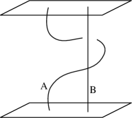
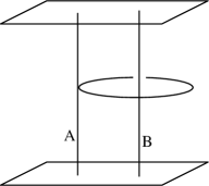
Figure 2: Adiabatic exchange of two particles A and B (left). This is topologically equivalent to the right configuration with linking number 1 and A will get gauge-transformed if B is the ’t Hooft operator.

Similarly, D6-brane baryon is a bound state of $N$ $Q^{\dagger}$’s, denoted by $(Q^{\dagger})^{N}$, which would be a singlet of $SU(N)$. Now the situation is totally opposite to the D2-brane baryon: it acquires $e^{2\pi iN/k}$ phase factor from $W_{4}$ but the trivial one from $T_{0}$, i.e., it detects $W_{4}$ but not $T_{0}$. We need to dress it by the $det(C)$–$W_{4}$ bound state to make anyon. Therefore, the $(Q^{\dagger})^{N}$–$det(C)$–$W_{4}$ bound states are the holographic anyons with the fractional phase equal to $n_{6}$ multiples of $2\pi N/k$ phase. Again, this fractional phase is captured by (3.10).

In summary: we assume the strings from the spiky D2 or D6 branes form the baryons, and by dressing them with the gauge invariant chiral primaries dual to the D0 or wrapped D4-branes, we can obtain the holographic anyons, with the fractional phases in agreement with the supergravity analysis.

Moreover, due to the non-trivial dressing, these holographic anyons may have less supersymmetry than the chiral primaries, and even are not BPS states. Since it is not clear how to check the BPS condition for such a composite operators, we will instead check it from their open string duals in the next section.

5 Constructing the holographic anyons

In this section, we describe supersymmetric D0- and D2-brane configurations in the ABJM background. The anyonic pair in the supergravity side can be constructed by these BPS configurations, though the bound states may break supersymmetry.

The Killing spinors in the ABJM background is summarized in the Appendix B. For our purpose in this section, it is more convenient to work in the Poincaré coordinate for $AdS_{4}$. Despite that, the Killing spinors given in (B.9)-(B.12) are still too complicated to be used to solve the kappa symmetry condition (B.17)-(B.19) for the BPS embedding of the D-branes. We have also tried to find BPS configurations of D4- and D6-branes, but have not made it. The setup and ansatz used there are also summarized in the Appendix C.

5.1 D0-brane

We start with considering D0-branes in the ABJM background and find the BPS configurations. In the ABJM paper, the chiral operators schematically represented as $C^{k}$ are identified with D0 brane in $AdS_{4}\times\mathbf{CP}^{3}$ background. These operators are in $\text{Sym}_{k}(\underline{\mathbf{4}})$ representation of $SU(4)_{R}$. In the gravity side, this $SU(4)_{R}$ corresponds to the isometry of $\mathbf{CP}^{3}$ and then BPS configuration would carry nontrivial angular momenta in $\mathbf{CP}^{3}$. We then consider D0 brane configurations rotating inside $\mathbf{CP}^{3}$. The Cartan subalgebras of $SU(4)_{R}$ correspond to the shifts in $\chi,\varphi_{1}$ and $\varphi_{2}$ coordinates and we thus turn on the angular momenta along these coordinates.

One-angular momentum case

First we consider a general configuration, where the D0 brane coordinates are given by $x=y=0$, $\theta_{1},\theta_{2},\alpha$ are all constant and $\varphi_{1}(t),\varphi_{2}(t),\chi(t)$ and $r(t)$ with the static gauge $\tau=t$. Then the action is given by

$$S_{D0}= T_{D0}e^{-\Phi}\int dt\sqrt{-\det g}-T_{D0}\int k\omega$$

$$= T_{D0}\frac{k}{2}\int dt\left[\sqrt{H}-\frac{1}{2}\cos\alpha\dot{\chi}-\cos^{2}\frac{\alpha}{2}\cos\theta_{1}\dot{\varphi}_{1}-\sin^{2}\frac{\alpha}{2}\cos\theta_{2}\dot{\varphi}_{2}\right]\,,$$ (5.1)

where

$$H= r^{2}-\frac{\dot{r}^{2}}{r^{2}}-A^{2}-B^{2}-C^{2}\,,$$ (5.2)

$$A= \sin\frac{\alpha}{2}\cos\frac{\alpha}{2}\left(\dot{\chi}+\cos\theta_{1}\dot{\varphi}_{1}-\cos\theta_{2}\dot{\varphi}_{2}\right)\,,$$ (5.3)

$$B= \cos\frac{\alpha}{2}\sin\theta_{1}\dot{\varphi}_{1}\,,$$ (5.4)

$$C= \sin\frac{\alpha}{2}\sin\theta_{2}\dot{\varphi}_{2}\,.$$ (5.5)

Obviously, constant $\dot{\chi},\dot{\varphi}_{1}$ and $\dot{\varphi}_{2}$ configuration solves the equation of motion and we will assume this.

The $\kappa$ symmetry projector is given by

$$\Gamma= \frac{1}{\sqrt{H}}\Gamma_{11}\left(r\Gamma_{0}-\frac{\dot{r}}{r}\Gamma_{3}+A\Gamma_{5}+B\Gamma_{7}+C\Gamma_{9}\right)\,,$$ (5.6)

and the BPS condition is that

$$\Gamma\epsilon= \epsilon\,,$$

$$\epsilon= \mathcal{K}\mathcal{L}\mathcal{M}\epsilon_{0}\,,$$ (5.7)

is solved by a constant spinor $\epsilon_{0}$. We first take $r(t)=r_{0}$. Inspired by the supersymmetry condition preserved by $M2$-branes generating this background, we may impose a projection condition,

$$\hat{\gamma}\Gamma_{3}\epsilon_{0}= \epsilon_{0}\,,$$ (5.8)

the Killing spinor is a bit simplified by $\mathcal{M}\epsilon_{0}=\epsilon_{0}$. After then we can take $r_{0}\rightarrow 0$ and then now D0 brane is sitting at the center of $AdS_{4}$.

Here we concentrate on the simplest case where only one of $A$, $B$ or $C$ is non-zero. All the cases go in parallel and then we consider $B=C=0$, that is, $\dot{\varphi}_{1}=\dot{\varphi}_{2}=0$ case. In this case the BPS condition is simplified to be

$$i\Gamma_{5}\Gamma_{11}\mathcal{K}\mathcal{L}\epsilon_{0}= \mathcal{K}\mathcal{L}\epsilon_{0}\,.$$ (5.9)

When $\theta_{1}=\theta_{2}=0$, $\Gamma_{5}\Gamma_{11}$ commutes with $\mathcal{K}$ and then we need to solve

$$i\Gamma_{5}\Gamma_{11}\mathcal{L}\epsilon_{0}= \mathcal{L}\epsilon_{0}\,.$$ (5.10)

By commuting $\Gamma_{5}\Gamma_{11}$ with $\mathcal{L}$, we finally arrive at

$$i\Gamma_{5}\Gamma_{11}e^{-\frac{\chi}{4}(\hat{\gamma}\Gamma_{11}-\Gamma_{45})}\epsilon_{0}= \epsilon_{0}\,.$$ (5.11)

We then impose the further projection conditions

$$i\Gamma_{5}\Gamma_{11}\epsilon_{0}= \epsilon_{0}\,,\qquad\hat{\gamma}\Gamma_{11}\epsilon_{0}=\Gamma_{45}\epsilon_{0}\,,$$ (5.12)

to solve the BPS condition. Let us count the number of the supersymmetry preserved by this D0-brane. Together with the previous projection condition and (B.15), we have imposed the conditions

$$\hat{\gamma}\Gamma_{3}\epsilon_{0}=\epsilon_{0}\,,\qquad\hat{\gamma}\Gamma_{11}\epsilon_{0}=\Gamma_{45}\epsilon_{0}\,,\qquad\Gamma_{67}\epsilon_{0}=\Gamma_{89}\epsilon_{0}\,,$$

$$i\Gamma_{5}\Gamma_{11}\epsilon_{0}=\epsilon_{0}\,.$$ (5.13)

So this configuration is a $1/6$ BPS configuration.

5.2 D2-branes

Since the wrapped D2-branes carry RR 2-form charges which should be canceled by the fundamental strings extending to the infinity. Similar story happened before for the wrapped D5-brane as the dual baryons proposed in [23]. Soon it was realized that the whole configuration can be realized as a spiky branes [24, 25] in AdS space, quite similar to its flat space counterpart considered in [21, 22]. Moreover, this configuration is BPS, in contrast to the non-BPS one considered in [26] by simply attached the fundamental strings to the wrapped branes. Following the same reasoning, it suggests that D2-brane wrapping on $\mathbf{CP}^{1}$ with $k$-strings attached and D6-brane wrapping on the whole $\mathbf{CP}^{3}$ with $N$-strings attached will be BPS when we replace the bunch of strings with a “spike” solutions on the DBI action [20]. We now construct the BPS spiky D2-branes here. However, we also find that the spiky D2 with magnetic flux satisfying (3.3) does not solve the equations of motion. Thus, we cannot have holographic anyon only from the spiky D2, instead we need to use the bound states such as the ones of spiky D2 and D4 with magnetic flux satisfying (3.2). Though this kind of holographic anyons could be unstable.

Ansatz

Suppose the D2-brane is wrapping on $\mathbf{CP}^{1}$ given by $\alpha=0$ slice of the $\mathbf{CP}^{3}$ and has a spike sourced by $k$-unit of the electric charge. The $\mathbf{CP}^{1}$ is parameterized as

$$ds^{2}_{CP^{1}}=\frac{1}{4}\left(d\theta_{1}^{2}+\sin^{2}\theta_{1}d\varphi_{1}^{2}\right)\,,$$ (5.14)

and because of the factor $4$ in (B.1), now $AdS_{4}$ and $\mathbf{CP}^{1}$ has the same radius. We take the static gauge

$$\tau=t\,,\qquad\sigma_{1}=\theta_{1}\,,\qquad\sigma_{2}=\varphi_{1}\,,$$ (5.15)

and the brane configuration is assumed to be given by $r(\theta_{1})$. We also turn on fluxes on the D2-brane, to be generic we have both electric and magnetic fluxes

$$\mathcal{F}= 2\pi\alpha^{\prime}F$$

$$= E^{1}d\tau\wedge d\sigma^{1}+E^{2}d\tau\wedge d\sigma^{2}+Bd\sigma^{1}\wedge d\sigma^{2}\,.$$ (5.16)

The DBI part of the action is

$$S_{DBI}= T_{D2}\int e^{-\Phi}\sqrt{-\det(g+2\pi\alpha^{\prime}F)}$$

$$= T_{D2}\frac{k}{2}\tilde{R}^{2}\int dtd\theta_{1}d\varphi_{1}\,\sqrt{H}\,,$$ (5.17)

$$H= \sin^{2}\theta_{1}\left(r^{2}+r^{\prime 2}\right)+r^{2}\mathbf{B}^{2}-\sin^{2}\theta_{1}\mathbf{E}_{1}^{2}-\left(1+\frac{r^{\prime 2}}{r^{2}}\right)\mathbf{E}_{2}^{2}\,,$$ (5.18)

where $\mathbf{B}=B/\tilde{R}^{2}$ etc. This D2-brane also coupled to the background RR 2-form flux,

$$S_{WZ}= -T_{D2}\int\mathcal{F}\wedge k\omega$$

$$= -T_{D2}\frac{k}{2}\tilde{R}^{2}\int\mathbf{E}_{1}\cos\theta_{1}dtd\theta_{1}d\varphi_{1}\,.$$ (5.19)

Thus the equations of motions are

$$0= \partial_{t}\left(\frac{\sin^{2}\theta_{1}}{\sqrt{H}}\mathbf{E}_{1}\right)-\partial_{\varphi_{1}}\left(\frac{r^{2}\mathbf{B}}{\sqrt{H}}\right)\,,$$ (5.20)

$$0= \partial_{t}\left(\frac{1+\frac{r^{\prime 2}}{r^{2}}}{\sqrt{H}}\mathbf{E}_{2}\right)+\partial_{\theta_{1}}\left(\frac{r^{2}\mathbf{B}}{\sqrt{H}}\right)\,,$$ (5.21)

$$0= -\partial_{\theta_{1}}\left(\frac{\sin^{2}\theta_{1}}{\sqrt{H}}\mathbf{E}_{1}+\cos\theta_{1}\right)-\partial_{\varphi_{1}}\left(\frac{1+\frac{r^{\prime 2}}{r^{2}}}{\sqrt{H}}\mathbf{E}_{2}\right)\,,$$ (5.22)

$$0= \partial_{\theta_{1}}\left(\frac{r^{\prime}\sin^{2}\theta_{1}-\frac{r^{\prime}}{r}\mathbf{E}_{2}^{2}}{\sqrt{H}}\right)-\frac{r\sin^{2}\theta_{1}+r\mathbf{B}^{2}+\frac{r^{\prime 2}}{r^{3}}\mathbf{E}_{2}^{2}}{\sqrt{H}}\,.$$ (5.23)

$\kappa$-symmetry Projector

For this D2-brane configuration, $\kappa$-symmetry projector becomes

$$\Gamma= \frac{1}{\sqrt{H}}\left[r\sin\theta_{1}\Gamma_{067}-r^{\prime}\sin\theta_{1}\Gamma_{037}+\sin\theta_{1}\mathbf{E}_{1}\Gamma_{7}\Gamma_{11}-\mathbf{E}_{2}\Gamma_{6}\Gamma_{11}+\frac{r^{\prime}}{r}\mathbf{E}_{2}\Gamma_{3}\Gamma_{11}-\mathbf{B}r\Gamma_{0}\Gamma_{11}\right]\,.$$ (5.24)

Now the BPS equation reads

$$\Gamma\mathcal{K}\mathcal{L}\epsilon_{0}= \mathcal{K}\mathcal{L}\epsilon_{0}\,,$$ (5.25)

where we have already assumed $\hat{\gamma}\Gamma_{3}\epsilon_{0}=\epsilon_{0}$. First consider

$$\mathcal{K}^{-1}\Gamma\mathcal{K}= \frac{1}{\sqrt{H}}\left[\left(r\sin\theta_{1}\Gamma_{067}-r^{\prime}\sin\theta_{1}\Gamma_{037}-\mathbf{E}_{2}\Gamma_{6}\Gamma_{11}+\frac{r^{\prime}}{r}\mathbf{E}_{2}\Gamma_{3}\Gamma_{11}+\mathbf{B}r\Gamma_{0}\Gamma_{11}\right)e^{-\frac{\theta_{1}}{2}(\hat{\gamma}\Gamma_{6}-\Gamma_{7}\Gamma_{11})}\right.$$

$$\left.\hskip 28.45274pt+\mathbf{E}_{1}\sin\theta_{1}\Gamma_{7}\Gamma_{11}\right]\,,$$ (5.26)

where we have used $\alpha=\theta_{2}=0$.

We here assume the following projection conditions on the constant spinor $\epsilon_{0}$,

$$\hat{\gamma}\Gamma_{3}\epsilon_{+}= \Gamma^{012}\epsilon_{0}=\epsilon_{0}\,,$$ (5.27)

$$\Gamma_{067}\epsilon_{0}= u\epsilon_{0}\,,$$ (5.28)

$$\Gamma_{03}\Gamma_{11}\epsilon_{0}= v\epsilon_{0}\,,$$ (5.29)

where $u$ and $v$ are $\pm 1$. The reason is the following. The first condition is the SUSY condition for the background $N$ M2-branes (or $N$ D2-branes) in the flat spacetime, and we have already imposed this condition for $t$-independence. The next condition is a (local) BPS condition for D2-branes wrapping on $\mathbf{CP}^{1}$ whose tangent space is given by $6,7$ directions. The last one is the BPS condition for the fundamental string stretching along the $r$-direction. With this ansatz, it is easy to see that

$$\mathcal{L}\epsilon_{0}= e^{\frac{\varphi_{1}}{4}(v-u)\Gamma_{0}}\epsilon_{0}\,.$$ (5.30)

When $\mathbf{B}=0$ or $u=v$, this factor is commuting with $\mathcal{K}^{-1}\Gamma\mathcal{K}$ and decouples from the BPS equation. Next consider $e^{-\frac{\theta_{1}}{2}(\hat{\gamma}\Gamma_{6}-\Gamma_{7}\Gamma_{11})}\epsilon_{0}$ part. Note that this factor commutes with $\mathcal{L}$ now. Under the projection condition, it becomes

$$e^{-\frac{\theta_{1}}{2}(\hat{\gamma}\Gamma_{6}-\Gamma_{7}\Gamma_{11})}\epsilon_{0}= e^{-\frac{\theta_{1}}{2}(1-uv)\Gamma_{36}}\epsilon_{0}\,.$$ (5.31)

So we assume $u=v$ and then can take $\mathcal{L}=1$. Further employing the projection conditions, the BPS equation becomes

$$\left[ur\sin\theta_{1}-\sqrt{H}-(vr^{\prime}-\mathbf{E}_{1})\sin\theta_{1}\Gamma_{7}\Gamma_{11}-\mathbf{E}_{2}\Gamma_{6}\Gamma_{11}+\frac{r^{\prime}}{r}\mathbf{E}_{2}\Gamma_{3}\Gamma_{11}+\mathbf{B}r\Gamma_{0}\Gamma_{11}\right]\epsilon_{0}=0\,.$$ (5.32)

Since $\Gamma_{6}\Gamma_{11},\Gamma_{7}\Gamma_{11}$ and $\Gamma_{0}\Gamma_{11}$ are not commuting with the projection conditions, we need to set all the coefficients to be zero, that is, $\mathbf{E}_{2}=\mathbf{B}=0$ and

$$\mathbf{E}_{1}=vr^{\prime}\,.$$ (5.33)

The rest condition is

$$ur\sin\theta_{1}=\sqrt{H}\,,$$ (5.34)

and this can be solved by $u=1$. In order to fix the profile of the spike, we then consider the equations of motion. The first two equations (5.20) and (5.21) are trivially satisfied. The last two equations (5.22) and (5.23) lead the same equation

$$\partial_{\theta_{1}}\left(\frac{r^{\prime}}{r}\sin\theta_{1}\right)=\sin\theta_{1}\,,$$ (5.35)

which can easily be integrated and the solution is given by

$$r(\theta_{1})= C_{1}\frac{1}{\sin\theta_{1}}\left(\frac{1-\cos\theta_{1}}{\sin\theta_{1}}\right)^{C_{2}}\,.$$ (5.36)

Here, one of the integration constant $C_{2}$ will be set to one in the following by the plausible flux distribution, and the other $C_{1}$ is the free moduli parameter for the radial position of the wrapped D2. Even though there is no BPS solution for $\mathbf{B}\neq 0$ case, one may wonder if there is non-BPS solution for it. However, it turns out that there is no spike solution of equations of motion for $\mathbf{E}_{2}=0$ but $\mathbf{B}\neq 0$ satisfying (3.3), i.e., $\mathbf{B}={m_{2}\over 2}\sin\theta_{1}$. To see this, one can first solve $\mathbf{E}_{1}$ from (5.22), and $\mathbf{B}$ is also given, then one can show that the remaining two equations (5.21) and (5.23) are not consistent with each other in solving the spike profile $r(\theta_{1})$.

Note that by giving up on having a spike we can obtain a solution to the equations of motion with a magnetic field. To see this, first notice that we need to introduce $k$ charges corresponding to the attached fundamental strings, as $k\delta^{2}(x)$ term in the Wess-Zumino term. Having this term allows us to set $A_{0}=\text{const.}$ consistently and then we have $\mathbf{E}=0$. Then together with $r=\text{const.}$, one finds that $\mathbf{B}\propto\cos\theta_{1}$ solves the equations of motion.

Distribution of the electric flux

In order to see Gauss law part of the equation of motion, it is useful to rewrite the action using explicitly $A_{\tau}$. We first consider the case with $\mathbf{E}_{2}=0$, $\mathbf{B}=0$ and $\mathbf{E}_{1}=-\tilde{R}^{-2}2\pi\alpha^{\prime}\partial_{\theta_{1}}A_{t}$. Then the $A_{t}$ equation of motions is

$$\partial_{\theta_{1}}\Pi_{\theta_{1}}= T_{D2}\frac{k}{2}2\pi\alpha^{\prime}\sin\theta_{1},,$$ (5.37)

$$\Pi_{\theta_{1}}= -T_{D2}\frac{k}{2}2\pi\alpha^{\prime}\frac{\sin\theta_{1}\mathbf{E}_{1}}{\sqrt{r^{2}+r^{\prime 2}-\mathbf{E}_{1}^{2}}}\,,$$ (5.38)

where

$$\Pi_{i}= \frac{\partial\mathcal{L}}{\partial(\partial_{i}A_{t})}$$ (5.39)

is the conjugate momentum. This corresponds to Gauss law $\nabla\cdot\mathbf{E}=\rho$ part of the Maxwell equations and the integration of $\Pi$ defines a conserved quantity and then integration of the right hand side over the spatial volume (now $\mathbf{CP}^{1}$) should give the total charge.

We here take the BPS spike solution,

$$r(\theta_{1})= C_{1}\frac{1}{\sin\theta_{1}}\left(\frac{1-\cos\theta_{1}}{\sin\theta_{1}}\right)^{C_{2}}\,,$$

$$\mathbf{E}_{1}= r^{\prime}\,,\quad\rightarrow\quad A_{t}(\theta_{1})=r\,,$$ (5.40)

and we obtain

$$\Pi_{\theta_{1}}= -\frac{k}{4\pi}(C_{2}-\cos\theta_{1})\,.$$ (5.41)

First we see the profile of the solution. For $\theta_{1}$ goes to $\pi$, both of $r(\theta_{1})$ and $A_{t}$ get divergent and then we conclude that the point charge is located at $\theta_{1}=\pi$. Next for small $\theta_{1}$, both of $r(\theta_{1})$ and $A_{t}$ behave as $\theta_{1}^{C_{2}-1}$. Therefore for the solution to be smooth on the other side of the spike, $C_{2}\geq 1$. Finally, by integrating $\Pi$ over $\mathbf{CP}^{1}$ we find

$$\int\sin\theta_{1}d\theta_{1}d\varphi_{1}\Pi_{\theta_{1}}= -C_{2}k\,.$$ (5.42)

This charge has to cancel the $k$ units of charge induced by the background, and therefore we get $C_{2}=1$. Thus the correct BPS solution with a plausible profile is given by

$$r(\theta_{1})= A_{t}(\theta_{1})=\frac{2r_{0}}{1+\cos\theta_{1}}\,,$$ (5.43)

where $r_{0}=C_{1}/2$ denote the position of the end of the spike at $\theta=0$, i.e., the radial position of the wrapped D2-brane.

We then conclude that each D0-brane having an angular momentum and D2-brane with a spike is a BPS configuration. It however turned out that, within our ansatz, the preserved supersymmetry by D0 and D2 branes are not compatible. Furthermore there does not exist BPS spike D2-branes with magnetic fluxes. These facts imply that our dressed baryons, D0-D2 bound states, are not BPS.

6 Conclusion and Discussions

In this paper, we have constructed the holographic anyons in the ABJM theory from the gravity, CFT and open string sides via AdS/CFT correspondence. The construction is more subtle than naively expected in all three aspects because it is the nontrivial generalization of the usual anyon constructed in the $U(1)$ Chern-Simons effective theory. In $U(1)$ case we attach the magnetic flux to the electron to make it anyon via the Chern-Simons coupling. Similarly, here we attach the nonabelian ’t Hooft operator to the baryon to make it anyonic.

We find two types of holographic anyons as the dressed baryons. One is the D0-D2 bound states, and the other is the D4-D6 ones. The anyonic phases from gravity and CFT sides agree. For D4-D6, the anyonic phase is proportional to the ’t Hooft coupling, and for D0-D2 its inverse. Interestingly, these two pairs are not related by the usual Hodge duality in ten dimensions, since it relates $C_{1}$ to $C_{7}$ and $C_{3}$ to $C_{5}$ but in the relation above the roles of D0 brane and D4 brane are exchanged. It has been suggested that this relation can be understood as a kind of geometric duality inside $\mathbf{CP}^{3}$[16]. Moreover, by combing with the level rank duality we can transform one anyonic phase to the other one, i.e.,

$$N\longleftrightarrow k\;,\qquad n_{0}\longleftrightarrow n_{4}\;,\qquad n_{2}\longleftrightarrow n_{6}\;,$$ (6.1)

and the anyonic phases are then switched as

$$n_{2}{2\pi k\over N}\longleftrightarrow n_{6}{2\pi N\over k}.$$ (6.2)

In the above, $n_{p}$ is the number of wrapped Dp-brane baryons in the anyon bound states. It is interesting to see if the combination of D0-D4 duality and level-rank duality is related to the particle-vortex duality in the quantum Hall system [27]. If this is the case, then D0-D2 and D4-D6 can be understood as the particle-vortex dual pair of CFT’s collective modes.

We also like to comment more on the agreement of the anyonic phases from gravity and CFT sides since it suggests that the anyonic phases do not run with the coupling constant. This seemingly topological feature should be due to the neglect of the interactions between the BPS Dp-branes if they are far enough from each other. Especially, in the supergravity side, if the distance between two branes (or strings and a brane) is not far enough, we may not be able to neglect the dynamical part of the phase, and as the separation distance goes to zero, the phase will disappear. This behavior might correspond to the fact in the field theory side that the ’t Hooft loops, or Wilson loops, become unstable once we introduce the fields which are not invariant under the center of the gauge group [13]. Therefore, the holographic anyonic phase is a long-range property of these pairs.

As a by product, we also examine the Killing spinor equation for the embedding branes wrapped over $\mathbf{CP}^{3}$. Though we have found the nontrivial BPS spiky wrapped D2-brane configuration, surprisingly some expected BPS solution for the chiral primary such as wrapped D4 brane and spiky D6 brane are not found by the simple ansatz based on symmetry argument. Despite that, we have put down the details of our unsuccessful trials and hopefully this will help for the further studies. We also note that though each of D0 brane and D2-brane with a spike is BPS, their bound state is not due to unmatching of the supersymmetries they preserve. It thus suggest that our dressed baryons are not protected from quantum corrections and it would appear very differently in either weak and strong coupling regimes. As noticed above, though, the anyonic phase (more precisely AB phase) between D0 and D2 are stable when the distance between them are far enough. It is then also interesting to investigate whether there exist BPS dressed baryon states in ABJM background.

We hope our results will inspire more studies on the connection between string theory and other branches of physics via AdS/CFT correspondence. It is also interesting to see if one can find the holographic anyons in the other holographic duals, and moreover, consider the dynamical consequences of these anyons, such as the implementation of topological quantum computing.

Appendix A Massive fluctuations

We will show that $F_{2}$ and $H_{3}$ are massive fields in the AdS bulk. This can seen most easily from the relevant field equations:

$$d*F_{2}-H_{3}+4\pi\delta^{3}(x)=0\;,$$ (A.1)

$$d*H_{3}+F_{2}=0\;.$$ (A.2)

From the above, we will obtain

$$d*d*H_{3}+H_{3}=4\pi\delta^{3}(x),$$ (A.3)

or

$$\Delta H_{3}-H_{3}=-4\pi\delta^{3}(x).$$ (A.4)

Obviously, it is a massive field, so is $F_{2}$.

Appendix B Killing spinors and supersymmetric embeddings

The ABJM geometry in the string frame metric ($\ell_{s}=1$) is

$$ds^{2}= \tilde{R}^{2}\left(ds^{2}_{AdS_{4}}+4ds^{2}_{\mathbf{CP}^{3}}\right)\,,$$ (B.1)

$$ds^{2}_{AdS_{4}}= r^{2}\left(-dt^{2}+dx^{2}+dy^{2}\right)+\frac{dr^{2}}{r^{2}}\,,$$ (B.2)

$$ds^{2}_{\mathbf{CP}^{3}}= \frac{1}{4}\left[d\alpha^{2}+\sin^{2}\frac{\alpha}{2}\cos^{2}\frac{\alpha}{2}\left(d\chi+\cos\theta_{1}d\varphi_{1}-\cos\theta_{2}d\varphi_{2}\right)^{2}\right.$$

$$\left.\hskip 28.45274pt+\cos^{2}\frac{\alpha}{2}\left(d\theta_{1}^{2}+\sin^{2}\theta_{1}d\varphi_{1}^{2}\right)\right.$$

$$\left.\hskip 28.45274pt+\sin^{2}\frac{\alpha}{2}\left(d\theta_{2}^{2}+\sin^{2}\theta_{2}d\varphi_{2}^{2}\right)\right]$$ (B.3)

$$(0\leq \alpha,\theta_{1},\theta_{2}\leq\pi\,,\qquad 0\leq\varphi_{1},\varphi_{2}<2\pi\,,\qquad 0\leq\chi<4\pi)$$ (B.4)

$$\tilde{R}^{2}= \frac{R^{3}}{4k}\,,\qquad\frac{R^{3}}{k}=2^{5/2}\pi\sqrt{N\over k}\,,$$ (B.5)

$$F_{4}= \frac{3}{8}R^{3}d\Omega_{AdS_{4}}\,,\quad F_{2}=kd\omega\,,\quad e^{2\Phi}=\frac{R^{3}}{k^{3}}\,,$$ (B.6)

$$\omega= \frac{1}{4}\left(\cos\alpha d\chi+2\cos^{2}\frac{\alpha}{2}\cos\theta_{1}d\varphi_{1}+2\sin^{2}\frac{\alpha}{2}\cos\theta_{2}d\varphi_{2}\right)\,.$$ (B.7)

In particular, we have chosen the Poincare coordinate for the $AdS_{4}$, which is more convenient for the Killing spinor analysis.

This background has the following vielbein:

$$e^{0}=\tilde{R}rdt\,,\qquad e^{1}=\tilde{R}rdx\,,\qquad e^{2}=\tilde{R}rdy\,,\qquad e^{3}=-\frac{\tilde{R}}{r}dr\,,$$

$$e^{4}=\tilde{R}d\alpha\,,\qquad e^{5}=\tilde{R}\sin\frac{\alpha}{2}\cos\frac{\alpha}{2}\left(d\chi+\cos\theta_{1}d\varphi_{1}-\cos\theta_{2}d\varphi_{2}\right)$$

$$e^{6}=\tilde{R}\cos\frac{\alpha}{2}d\theta_{1}\,,\qquad e^{7}=\tilde{R}\cos\frac{\alpha}{2}\sin\theta_{1}d\varphi_{1}$$

$$e^{8}=\tilde{R}\sin\frac{\alpha}{2}d\theta_{2}\,,\qquad e^{9}=\tilde{R}\sin\frac{\alpha}{2}\sin\theta_{2}d\varphi_{2}\,.$$ (B.8)

Killing spinor

This background turns out to have the following Killing spinor

$$\epsilon= \mathcal{K}\mathcal{L}\mathcal{M}\epsilon_{0}\,,$$ (B.9)

$$\mathcal{K}= e^{-\frac{\alpha}{4}(\hat{\gamma}\Gamma_{4}-\Gamma_{5}\Gamma_{11})}e^{-\frac{\theta_{1}}{4}(\hat{\gamma}\Gamma_{6}-\Gamma_{7}\Gamma_{11})+\frac{\theta_{2}}{4}(\Gamma_{4}\Gamma_{8}+\Gamma_{5}\Gamma_{9})}\,,$$ (B.10)

$$\mathcal{L}= e^{\xi_{1}\hat{\gamma}\Gamma_{11}+\xi_{2}\Gamma_{45}+\xi_{3}\Gamma_{67}+\xi_{4}\Gamma_{89}}\,,$$ (B.11)

$$\mathcal{M}= r^{1/2}\left[\frac{1+\hat{\gamma}\Gamma_{3}}{2}+\left(t\Gamma_{0}+x\Gamma_{1}+y\Gamma_{2}+\frac{1}{r}\Gamma_{3}\right)\Gamma_{3}\frac{1-\hat{\gamma}\Gamma_{3}}{2}\right]\,,$$ (B.12)

where

$$\xi_{1}=-\frac{\chi}{8}-\frac{\varphi_{1}}{4}\,,\quad\xi_{2}=\frac{\chi}{8}-\frac{\varphi_{2}}{4}\,,\quad\xi_{3}=-\frac{\chi}{8}+\frac{\varphi_{1}}{4}\,,\quad\xi_{4}=\frac{\chi}{8}+\frac{\varphi_{2}}{4}\,.$$ (B.13)

Note that

$${\cal M}\epsilon_{0}=\epsilon_{0}$$ (B.14)

if $\hat{\gamma}\Gamma_{3}\epsilon_{0}=\epsilon_{0}$.

And the dilatino condition gives projection condition for the constant spinor

$$(\hat{\gamma}\Gamma_{11}+\Gamma^{45}+\Gamma^{67}+\Gamma^{89})\epsilon_{0}=0\,.$$ (B.15)

Moreover, these four Gamma matrices commute with each other and have their squares to be $-1$ so we can choose

$$\hat{\gamma}\Gamma_{11}\epsilon_{0}=is_{0}\epsilon_{0},\qquad\Gamma_{45}\epsilon_{0}=is_{1}\epsilon_{0},\qquad\Gamma_{67}\epsilon_{0}=is_{2}\epsilon_{0},\qquad\Gamma_{89}\epsilon_{0}=is_{3}\epsilon_{0},$$ (B.16)

where $s_{i}\in{\pm 1}$ and satisfy $\sum_{i}s_{i}=0$ so that the background is found to preserve $\mathcal{N}=6$ supersymmetry. We can choose another matrix commuting with all of the above as $\hat{\gamma}\Gamma_{3}=\Gamma^{012}$. We may write the eigenvalue of this as $is_{5}$ and then the 32 component spinor is specified by the set of the eigenvalues $(s_{0},s_{1},s_{2},s_{3},s_{4},s_{5})$.

The projector

The $\kappa$-symmetry projector for a Dp-brane with world-volume gauge field strength $\mathcal{F}_{2}$ in a Lorentzian background is given in [18, 19] as

$$\Gamma= \frac{\sqrt{|g|}}{\sqrt{|g+\mathcal{F}|}}\sum_{n=0}^{\infty}\frac{1}{2^{n}n!}\gamma^{i_{1}j_{1}\cdots i_{n}j_{n}}\mathcal{F}_{i_{1}j_{1}}\cdots\mathcal{F}_{i_{n}j_{n}}J_{(p)}^{(n)}\,,$$ (B.17)

$$J_{(p)}^{(n)}= (\Gamma_{11})^{n+\frac{p-2}{2}}\Gamma_{(0)}\,,$$ (B.18)

$$\Gamma_{(0)}= \frac{1}{(p+1)!}\frac{1}{\sqrt{|g|}}\varepsilon^{i_{1}\cdots i_{p+1}}\gamma_{i_{1}\cdots i_{p+1}}\,,$$ (B.19)

where $i_{1},\cdots$ are the world-volume indices, $\gamma_{i}=\partial_{i}X^{\mu}\gamma_{\mu}$ is the pull-back of the curved-space gamma matrices $\gamma_{\mu}$ onto the world-volume, and $\gamma_{\mu}=e^{a}_{\mu}\Gamma_{a}$.

By using this projector, the BPS condition for the embedding is given by

$$\Gamma\epsilon=\epsilon\,.$$ (B.20)

Appendix C Some trial for BPS D4 and spiky D6 brane configurations

Apart from the D0 and D2-brane cases, we have also tried to solve the BPS conditions for D4 and D6-brane cases. Though we have not found BPS configurations, we here note our setup and ansatz for future reference.

C.0.1 D4-branes

We consider a D4-brane wrapping on $\mathbf{CP}^{2}$. In the original background given by $\mathbb{R}^{1,2}\times\mathbb{C}^{4}/\mathbb{Z}_{k}$, the would-be-$\mathbf{CP}^{2}$ can be regarded as a flat three plane through the origin of $\mathbb{C}^{4}$. We then take $z_{4}=0$, which leads $\mathbf{CP}^{2}:\,\theta_{2}=0\,,\quad\varphi_{2}=0$.

The configuration we consider is

	$t$	$x$	$y$	$r$	$\alpha$	$\chi$	$\theta_{1}$	$\varphi_{1}$	$\theta_{2}$	$\varphi_{2}$
D4	$\circ$			$r$	$\circ$	$\circ$	$\circ$	$\circ$	$0$	$0$

with $F_{\alpha\chi}$ and $F_{\theta_{1}\varphi_{1}}$ turned on. Thus the DBI action is

$$S_{D4,DBI}=T_{D_{4}}\tilde{R}^{5}\frac{k}{2\tilde{R}}\int dtd\alpha d\chi d\theta_{1}d\varphi_{1}\,r\,\cos^{3}\frac{\alpha}{2}\sin\frac{\alpha}{2}\sin\theta_{1}\sqrt{H}\,,$$ (C.1)

where

$$H:= (1+B_{1}^{2})(1+B_{2}^{2})\;,\qquad B_{1}=\frac{2\pi\alpha^{\prime}\,F_{\alpha\chi}}{\tilde{R}^{2}\cos\frac{\alpha}{2}\sin\frac{\alpha}{2}}\,,\qquad B_{2}= \frac{2\pi\alpha^{\prime}\,F_{\theta_{1}\varphi_{1}}}{\tilde{R}^{2}\cos^{2}\frac{\alpha}{2}\sin\theta_{1}}\,.$$ (C.2)

Since we have not turned on any electric fields on D4-brane, the Wess-Zumino term does not exist.

The equations of motion of $B_{1}$ and $B_{2}$ are reduced to

$$\partial_{\alpha}\left(\cos^{2}\frac{\alpha}{2}\frac{B_{1}(1+B_{2}^{2})}{\sqrt{H}}\right)=0\,,\qquad\partial_{\theta_{1}}\left(\frac{B_{2}(1+B_{1}^{2})}{\sqrt{H}}\right)=0\,.$$ (C.3)

These equations are solved by

$$B_{1}^{2}={C_{1}^{2}(C_{2}^{2}-1)\over C_{1}^{2}-\cos^{4}{\alpha\over 2}}\;,\qquad B_{2}^{2}={C_{2}^{2}\over C_{2}^{2}-1}({C_{1}^{2}\over\cos^{4}{\alpha\over 2}}-1)$$ (C.4)

where $C_{1}(\theta_{1})$ is an arbitrary function of $\theta_{1}$ only, and $C_{2}(\alpha)$ depends only on $\alpha$, instead.

BPS conditions

The $\Gamma$ projector is given by

$$\Gamma=\frac{1}{\sqrt{H}}\left((\Gamma_{11}\Gamma_{45}-B_{1})\Gamma_{067}(1-\sin{\alpha\over 2}\cot\theta_{1}\Gamma_{57})-B_{2}\Gamma_{045}+B_{1}B_{2}\Gamma_{11}\Gamma_{0}\right)$$ (C.5)

and the kappa symmetry condition

$$\Gamma{\cal KL}\epsilon_{0}={\cal KL}\epsilon_{0}$$ (C.6)

where we have chosen the projection condition $\hat{\gamma}\Gamma_{3}\epsilon_{0}=\epsilon_{0}$ such that ${\cal M}\epsilon_{0}=\epsilon_{0}$.

We then assume the following projection condition

$$\hat{\gamma}\Gamma_{11}\epsilon_{0}= \beta_{1}\Gamma_{45}\epsilon_{0}=\beta_{2}\Gamma_{67}\epsilon_{0}=\beta_{3}\Gamma_{89}\epsilon_{0}$$ (C.7)

and $\beta_{i}=\pm 1$ and the dilatino condition (B.15) requires that $\beta_{1}+\beta_{2}+\beta_{3}=-1$. Then we find that

$$\mathcal{L}\epsilon_{0}= e^{(\beta_{3}\xi_{1}+\beta_{1}\beta_{3}\xi_{2}+\beta_{2}\beta_{3}\xi_{3}+\xi_{4})\Gamma_{89}}\epsilon_{0}\,,$$ (C.8)

and since $\Gamma_{89}$ commutes with both of $\mathcal{M}$ and $\Gamma$, in (C.6) the $\mathcal{L}$ part trivially cancel on the both hands sides.

We then need to commute $\Gamma$ with ${\cal K}$ to solve the BPS condition. After some algebra, we arrive at

$$\sqrt{H}\mathcal{K}^{-1}\Gamma\mathcal{K}$$

$$= -\Gamma_{0}\Gamma_{11}\Gamma_{4567}\left(1-\sin\frac{\alpha}{2}\cot\theta_{1}\left(\cos\frac{\alpha}{2}\Gamma_{57}e^{\frac{\theta_{1}}{2}\Gamma_{7}\Gamma_{11}}-\sin\frac{\alpha}{2}\Gamma_{7}\Gamma_{11}\right)\right)$$

$$-B_{1}\Gamma_{067}\left(1+\sin^{2}\frac{\alpha}{2}\cot\theta_{1}\Gamma_{7}\Gamma_{11}\right)e^{-\frac{\theta_{1}}{2}(\hat{\gamma}\Gamma_{6}-\Gamma_{7}\Gamma_{11})}$$

$$+B_{1}\Gamma_{056}\sin\frac{\alpha}{2}\cos\frac{\alpha}{2}\cot\theta_{1}e^{-\frac{\theta_{1}}{2}\hat{\gamma}\Gamma_{6}}$$

$$-B_{2}\Gamma_{045}\left(\cos\frac{\alpha}{2}-\sin\frac{\alpha}{2}\hat{\gamma}\Gamma_{4}e^{-\frac{\theta_{1}}{2}\hat{\gamma}\Gamma_{6}}\right)\left(\cos\frac{\alpha}{2}+\sin\frac{\alpha}{2}\Gamma_{5}\Gamma_{11}e^{\frac{\theta_{1}}{2}\Gamma_{7}\Gamma_{11}}\right)$$

$$-B_{1}B_{2}\Gamma_{0}\Gamma_{11}\left(\cos\frac{\alpha}{2}-\sin\frac{\alpha}{2}\hat{\gamma}\Gamma_{4}e^{\frac{\theta_{1}}{2}\hat{\gamma}\Gamma_{6}}\right)\left(\cos\frac{\alpha}{2}+\sin\frac{\alpha}{2}\Gamma_{5}\Gamma_{11}e^{-\frac{\theta_{1}}{2}\Gamma_{7}\Gamma_{11}}\right)e^{-\frac{\theta_{1}}{2}(\hat{\gamma}\Gamma_{6}-\Gamma_{7}\Gamma_{11})}\,.$$ (C.9)

Let us first consider $(\beta_{1},\beta_{2},\beta_{3})=(-,+,-)$ case. For this choice, the BPS equation becomes

$$\epsilon_{0}= \frac{1}{\sqrt{H}}\left[-(1+B_{1}B_{2}\cos\alpha)\Gamma_{0}\Gamma_{11}-B_{1}\sin^{2}\frac{\alpha}{2}\cot\theta_{1}\Gamma_{0457}\Gamma_{11}\right.$$

$$+\left(\cos\frac{\alpha}{2}\sin\frac{\alpha}{2}\cot\theta_{1}\cos\frac{\theta_{1}}{2}-B_{1}B_{2}\sin\alpha\sin\frac{\theta_{1}}{2}\right)\Gamma_{057}\Gamma_{11}$$

$$-\left(B_{1}\cos\frac{\alpha}{2}\sin\frac{\alpha}{2}\cot\theta_{1}\sin\frac{\theta_{1}}{2}+B_{2}\sin\alpha\cos\frac{\theta_{1}}{2}\right)\Gamma_{04}\Gamma_{11}$$

$$+\left(\cos\frac{\alpha}{2}\sin\frac{\alpha}{2}\cot\theta_{1}\sin\frac{\theta_{1}}{2}+B_{1}B_{2}\sin\alpha\cos\frac{\theta_{1}}{2}\right)\Gamma_{05}$$

$$-\sin^{2}\frac{\alpha}{2}\cot\theta_{1}\Gamma_{07}+(B_{1}-B_{2}\cos\alpha)\Gamma_{045}$$

$$\left.+\left(B_{1}\cos\frac{\alpha}{2}\sin\frac{\alpha}{2}\cot\theta_{1}\cos\frac{\theta_{1}}{2}-B_{2}\sin\alpha\sin\frac{\theta_{1}}{2}\right)\Gamma_{056}\right]\epsilon_{0}$$ (C.10)

We have $\Gamma_{07}$ term whose coefficient does not include $B$’s. For BPS solutions to exist, this $\Gamma_{07}$ should be projected to be either $\mathbf{1}$ or one of the other gamma matrices. However, any of this choice will not be compatible with the projection conditions we have already imposed and then will break all the supersymmetry. We thus see that there is no BPS solution. We have also checked the other two cases, $(\beta_{1},\beta_{2},\beta_{3})=(+,-,-)$ and $(\beta_{1},\beta_{2},\beta_{3})=(-,-,+)$, and have arrived at the same structure and not found any BPS configuration based on this ansatz.

C.0.2 $\mathbf{CP}^{1}\times\mathbf{CP}^{1}$ embedding

By setting $\theta_{1}=\theta_{2}:=\theta$ and $\varphi_{1}=\varphi_{2}:=\varphi$, the $\mathbf{CP}^{3}$ is reduced to $\mathbf{CP}^{1}\times\mathbf{CP}^{1}$ of the equal radius, we then wrap D4-brane on it.

We may turn on two independent magnetic fields $F_{\alpha\tilde{\chi}}$ and $F_{\theta\varphi}$ and then the action is (Wess-Zumino part again vanishes)

$$S_{D4,DBI}= T_{D_{4}}\int e^{-\Phi}\sqrt{-\det(g+\mathcal{F})}$$

$$= T_{D_{4}}\tilde{R}^{5}\frac{k}{2\tilde{R}}\int d\alpha d\tilde{\chi}d\theta d\varphi\,r\,\sin\alpha\sin\theta\sqrt{H}\,,$$ (C.11)

$$B_{1}=\frac{2\pi\alpha^{\prime}F_{\alpha\tilde{\chi}}}{\tilde{R}^{2}\sin\alpha}\,,\qquad B_{2}=\frac{2\pi\alpha^{\prime}F_{\theta\varphi}}{\tilde{R}^{2}\sin\theta}\,,$$ (C.12)

where $\tilde{\chi}=\chi/2$ and $H$ is the same as (C.2).

The equations of motion are (by choosing the gauge $F_{\alpha\tilde{\chi}}=\partial_{\alpha}A_{\tilde{\chi}}$ and $F_{\theta\varphi}=\partial_{\theta}A_{\varphi}$)

$$\partial_{\alpha}\left(\frac{B_{1}(1+B_{2}^{2})}{\sqrt{H}}\right)=0\,,\qquad\partial_{\theta_{1}}\left(\frac{B_{2}(1+B_{1}^{2})}{\sqrt{H}}\right)=0\,.$$ (C.13)

These are solved by

$$B_{1}^{2}={C_{1}^{2}\over 1-C_{1}^{2}}\;,\qquad B_{2}^{2}={C_{2}^{2}\over 1-C_{2}^{2}}\;,$$ (C.14)

where $C_{1}=C_{1}(\theta)$, $C_{2}=C_{2}(\alpha)$ are arbitrary functions.

The $\Gamma$ projector is then given by

$$\Gamma={1\over\sqrt{H}}(\Gamma_{11}\Gamma_{045\tilde{6}\tilde{7}}-B_{1}\Gamma_{0\tilde{6}\tilde{7}}-B_{2}\Gamma_{045}+B_{1}B_{2}\Gamma_{11}\Gamma_{0})\;,$$ (C.15)

where

$$\Gamma_{\tilde{6}}:=\cos{\alpha\over 2}\Gamma_{6}+\sin{\alpha\over 2}\Gamma_{8}\;,\qquad\Gamma_{\tilde{7}}:=\cos{\alpha{}\over 2}\Gamma_{7}+\sin{\alpha{}\over 2}\Gamma_{9}\;.$$ (C.16)

We will impose $\hat{\gamma}\Gamma_{3}\epsilon_{0}=\epsilon_{0}$ condition as before. We need to impose further conditions for simplicity. The simplest projection condition here is to choose

$$\hat{\gamma}\Gamma_{11}\epsilon_{0}= -\Gamma_{45}\epsilon_{0}=-\Gamma_{67}\epsilon_{0}=\Gamma_{89}\epsilon_{0}\,,$$ (C.17)

which leads $\mathcal{L}\epsilon_{0}=\epsilon_{0}$. With this choice, $\mathcal{K}=e^{-\frac{\alpha}{4}(\hat{\gamma}\Gamma_{4}-\Gamma_{5}\Gamma_{11})}e^{-\frac{\theta}{2}(\hat{\gamma}\Gamma_{6}-\Gamma_{48})}$ on $\epsilon_{0}$, and then BPS equation is reduced to

$$\epsilon_{0}= \frac{\Gamma_{0}}{\sqrt{H}}\left[\left\{e^{-\theta\Gamma_{48}}\left(\cos^{2}\frac{\alpha}{2}+\sin^{2}\frac{\alpha}{2}B_{1}B_{2}\right)-e^{\theta\hat{\gamma}\Gamma_{6}}\left(\sin^{2}\frac{\alpha}{2}+\cos^{2}\frac{\alpha}{2}B_{1}B_{2}\right)\right\}\Gamma_{11}\right.$$

$$\hskip 56.9055pt+\left\{e^{-\theta\Gamma_{48}}\left(\sin^{2}\frac{\alpha}{2}B_{1}-\cos^{2}\frac{\alpha}{2}B_{2}\right)-e^{\theta\hat{\gamma}\Gamma_{6}}\left(\cos^{2}\frac{\alpha}{2}B_{1}-\sin^{2}\frac{\alpha}{2}B_{2}\right)\right\}\Gamma_{45}$$

$$\hskip 56.9055pt\left.+\sin\frac{\alpha}{2}\cos\frac{\alpha}{2}\left(e^{-\theta\Gamma_{48}}+e^{\theta\hat{\gamma}\Gamma_{6}}\right)\left(-\Gamma_{68}\Gamma_{11}+B_{1}\Gamma_{78}-B_{2}\Gamma_{4}\Gamma_{11}+B_{1}B_{2}\Gamma_{5}\right)\right]\epsilon_{0}\,.$$ (C.18)

Since the coefficient of $\Gamma_{68}\Gamma_{11}$ term does not involve $B_{1}$ nor $B_{2}$, this needs to be projected to either constant or another gamma matrix structure. However, it will not be compatible with the projection conditions above, and then we conclude that there is no BPS solution with these conditions.

In summary: We cannot find the BPS configuration for D4 branes wrapping on $\mathbf{CP}^{2}$ or $\mathbf{CP}^{1}\times\mathbf{CP}^{1}$ with magnetic fields turned on.

C.0.3 D6-brane

We now consider a D6-brane wrapping on the whole $\mathbf{CP}^{3}$ and having a spike. The ansatz we take is

	$t$	$x$	$y$	$r$	$\alpha$	$\chi$	$\theta_{1}$	$\varphi_{1}$	$\theta_{2}$	$\varphi_{2}$
D6	$\sigma^{0}$	$0$	$0$	$r(\alpha,\theta_{1},\theta_{2})$	$\sigma^{1}$	$\sigma^{2}$	$\sigma^{3}$	$\sigma^{4}$	$\sigma^{5}$	$\sigma^{6}$

with $E_{\alpha}=\tilde{R}^{-2}\mathcal{F}_{\sigma^{0}\sigma^{1}}\,,\,E_{1}=\tilde{R}^{-2}\mathcal{F}_{\sigma^{0}\sigma^{3}}\,,\,E_{2}=\tilde{R}^{-2}\mathcal{F}_{\sigma^{0}\sigma^{5}}$ turned on. Then

$$\sqrt{-\det(g+\mathcal{F})}= \tilde{R}^{7}\sin^{2}\frac{\alpha}{2}\cos^{2}\frac{\alpha}{2}\sin\theta_{1}\sin\theta_{2}\sqrt{H}\,,$$ (C.19)

$$H(r(\alpha))= r^{2}\left(1+\frac{r_{\alpha}^{2}}{r^{2}}\right)\left(c_{\alpha}^{2}+\frac{r_{1}^{2}}{r^{2}}\right)\left(s_{\alpha}^{2}+\frac{r_{2}^{2}}{r^{2}}\right)-E_{\alpha}^{2}\left(c_{\alpha}^{2}+\frac{r_{1}^{2}}{r^{2}}\right)\left(s_{\alpha}^{2}+\frac{r_{2}^{2}}{r^{2}}\right)$$

$$-E_{1}^{2}\left(1+\frac{r_{\alpha}^{2}}{r^{2}}\right)\left(s_{\alpha}^{2}+\frac{r_{2}^{2}}{r^{2}}\right)-E_{2}^{2}\left(1+\frac{r_{\alpha}^{2}}{r^{2}}\right)\left(c_{\alpha}^{2}+\frac{r_{1}^{2}}{r^{2}}\right)\,,$$ (C.20)

where $r_{\alpha}=\partial_{\alpha}r$, $r_{1,2}=\partial_{\theta_{1,2}}r$ and $c_{\alpha}=\cos\alpha/2,s_{\alpha}=\sin\alpha/2$.

The projector is given by

$$\Gamma= \frac{1}{\sin\theta_{1}\sin\theta_{2}\sqrt{H}}\Gamma_{I}\Gamma_{II}\,,$$

$$\Gamma_{I}= -r\Gamma_{0}\left(r\Gamma_{4}-\frac{r_{\alpha}}{r}\Gamma_{3}\right)\left(c_{\alpha}\Gamma_{6}-\frac{r_{1}}{r}\Gamma_{3}\right)\left(s_{\alpha}\Gamma_{8}-\frac{r_{2}}{r}\Gamma_{3}\right)+E_{\alpha}\left(c_{\alpha}\Gamma_{6}-\frac{r_{1}}{r}\Gamma_{3}\right)\left(s_{\alpha}\Gamma_{8}-\frac{r_{2}}{r}\Gamma_{3}\right)\Gamma_{11}$$

$$-E_{1}\left(r\Gamma_{4}-\frac{r_{\alpha}}{r}\Gamma_{3}\right)\left(s_{\alpha}\Gamma_{8}-\frac{r_{2}}{r}\Gamma_{3}\right)\Gamma_{11}+E_{2}\left(r\Gamma_{4}-\frac{r_{\alpha}}{r}\Gamma_{3}\right)\left(c_{\alpha}\Gamma_{6}-\frac{r_{1}}{r}\Gamma_{3}\right)\Gamma_{11}\,,$$

$$\Gamma_{II}= \Gamma_{5}\left(\sin\theta_{1}\Gamma_{7}+\sin\frac{\alpha}{2}\cos\theta_{1}\Gamma_{5}\right)\left(\sin\theta_{2}\Gamma_{9}-\cos\frac{\alpha}{2}\cos\theta_{2}\Gamma_{5}\right)\,.$$ (C.21)

We then impose the following projection conditions:

$$\hat{\gamma}\Gamma_{3}\epsilon_{0}= \epsilon_{0}\,,$$ (C.22)

$$\Gamma_{03}\Gamma_{11}\epsilon_{0}= v\epsilon_{0}\,,$$ (C.23)

$$\Gamma_{0456789}\epsilon_{0}= u\epsilon_{0}\,,$$ (C.24)

$$\hat{\gamma}\Gamma_{11}\epsilon_{0}= -\Gamma_{45}\epsilon_{0}=\Gamma_{67}\epsilon_{0}=-\Gamma_{89}\epsilon_{0}\,,$$ (C.25)

and by using the first two conditions, it is easy to see that $\mathcal{L}\epsilon_{0}=e^{v(-\xi_{1}+\xi_{2}-\xi_{3}+\xi_{4})\Gamma_{0}}\epsilon_{0}$ and since $\Gamma_{0}$ commutes with $\mathcal{K}$ and $\Gamma$, $\mathcal{L}$ will decouple from the BPS condition. $\mathcal{K}\epsilon_{0}$ is also simplified as $\mathcal{K}\epsilon_{0}=e^{-\frac{\alpha}{2}\hat{\gamma}\Gamma_{4}}\epsilon_{0}\equiv\mathcal{K}^{\prime}\epsilon_{0}$. Then

$$\Gamma_{I}\Gamma_{II}\mathcal{K}^{\prime}= \mathcal{K}^{\prime}\Gamma_{II}\left[-r\Gamma_{0}\left(\Gamma_{4}-\frac{r_{\alpha}}{r}\Gamma_{3}\right)\left(\frac{r_{2}}{r}c_{\alpha}\Gamma_{36}-\frac{r_{1}}{r}s_{\alpha}\Gamma_{38}\right)\right.$$

$$\left.\hskip 14.22636pt-\left\{E_{\alpha}c_{\alpha}s_{\alpha}\Gamma_{68}+E_{\alpha}\frac{r_{1}r_{2}}{r^{2}}+\left(\Gamma_{4}-\frac{r_{\alpha}}{r}\Gamma_{3}\right)\left(\frac{r_{2}}{r}E_{1}-\frac{r_{1}}{r}E_{2}\right)\Gamma_{3}\right\}\Gamma_{11}\right.$$

$$\left.+\left\{-r\Gamma_{0}\left(\Gamma_{4}-\frac{r_{\alpha}}{r}\Gamma_{3}\right)\left(c_{\alpha}s_{\alpha}\Gamma_{68}+\frac{r_{1}r_{2}}{r^{2}}\right)\right.\right.$$

$$\left.\left.-\left(-E_{\alpha}\left(\frac{r_{2}}{r}c_{\alpha}\Gamma_{63}+\frac{r_{1}}{r}s_{\alpha}\Gamma_{38}\right)+\left(\Gamma_{4}-\frac{r_{\alpha}}{r}\Gamma_{3}\right)(-E_{1}s_{\alpha}\Gamma_{8}+E_{2}c_{\alpha}\Gamma_{6})\right)\Gamma_{11}\right\}e^{-\alpha\hat{\gamma}\Gamma_{4}}\right]\,.$$ (C.26)

We then consider the last $[\cdots]$ factor on $\epsilon_{0}$. By applying the projection conditions, we have

$$\big{[}\cdots\big{]}(\text{on}\,\,\epsilon_{0})= \Gamma_{4}\left(\left(vr_{2}-E_{2}\cos\alpha-\frac{r_{\alpha}}{r}\sin\alpha E_{2}+\frac{r_{2}}{r}E_{\alpha}\sin\alpha\right)c_{\alpha}\Gamma_{6}\right.$$

$$\left.\hskip 10.00002pt-\left(vr_{1}-E_{1}\cos\alpha-\frac{r_{\alpha}}{r}\sin\alpha E_{1}+\frac{r_{1}}{r}E_{\alpha}\sin\alpha\right)s_{\alpha}\Gamma_{8}\right)\Gamma_{11}$$

$$+\left(-E_{\alpha}+vr_{\alpha}\cos\alpha-vr\sin\alpha\right)s_{\alpha}c_{\alpha}\Gamma_{68}\Gamma_{11}$$

$$+\frac{1}{r^{2}}\left(r_{\alpha}r_{2}E_{1}-r_{\alpha}r_{1}E_{2}-r_{1}r_{2}E_{\alpha}+vr_{\alpha}r_{1}r_{2}\cos\alpha-vrr_{1}r_{2}\sin\alpha\right)\Gamma_{11}$$

$$+\left\{\left(-\frac{r_{\alpha}r_{2}}{r}-v\frac{r_{2}}{r}E_{\alpha}\cos\alpha+v\frac{r_{\alpha}}{r}E_{2}\cos\alpha-vE_{2}\sin\alpha\right)c_{\alpha}\Gamma_{6}\right.$$

$$\left.\hskip 10.00002pt-\left(-\frac{r_{\alpha}r_{1}}{r}-v\frac{r_{1}}{r}E_{\alpha}\cos\alpha+v\frac{r_{\alpha}}{r}E_{1}\cos\alpha-vE_{1}\sin\alpha\right)s_{\alpha}\Gamma_{8}\right\}\Gamma_{0}$$

$$+\left(-v\frac{1}{r}(r_{2}E_{1}-r_{1}E_{2})-\frac{r_{1}r_{2}}{r}\cos\alpha-\frac{r_{\alpha}r_{1}r_{2}}{r^{2}}\sin\alpha\right)\Gamma_{04}$$

$$-(r\cos\alpha+r_{\alpha}\sin\alpha)s_{\alpha}c_{\alpha}\Gamma_{0468}\,.$$ (C.27)

Since $\Gamma_{II}$ are terms of $\Gamma_{5},\Gamma_{7}$ and $\Gamma_{9}$ and will not become terms with $\Gamma_{11}$ after projection conditions, we impose here all the terms proportional to $\Gamma_{11}$ to vanish and have

$$E_{\alpha}= v(r_{\alpha}\cos\alpha-r\sin\alpha)\,,\qquad E_{1}=vr_{1}\cos\alpha\,,\qquad E_{2}=vr_{2}\cos\alpha\,.$$ (C.28)

By plugging these solutions to the BPS equation again, we get

$$\epsilon_{0}=\frac{1}{\sin\theta_{1}\sin\theta_{2}\sqrt{H}}$$

$$\times\left[\left(\frac{r_{\alpha}r_{2}}{r}c_{\alpha}^{2}\sin\theta_{1}\cos\theta_{2}+\frac{r_{\alpha}r_{1}}{r}s_{\alpha}^{2}\cos\theta_{1}\sin\theta_{2}\right.\right.$$

$$\left.\hskip 20.00003pt+(r\cos\alpha+r_{\alpha}\sin\alpha)\left(-\frac{r_{1}r_{2}}{r^{2}}c_{\alpha}s_{\alpha}\cos\theta_{1}\cos\theta_{2}-c_{\alpha}s_{\alpha}\sin\theta_{1}\sin\theta_{2}\right)\right)\mathbf{1}$$

$$+\left(-\frac{r_{\alpha}r_{2}}{r}c_{\alpha}^{2}s_{\alpha}\cos\theta_{1}\cos\theta_{2}+\frac{r_{\alpha}r_{1}}{r}s_{\alpha}\sin\theta_{1}\sin\theta_{2}\right.$$

$$\left.\hskip 20.00003pt+(r\cos\alpha+r_{\alpha}\sin\alpha)\left(-\frac{r_{1}r_{2}}{r^{2}}c_{\alpha}\sin\theta_{1}\cos\theta_{2}+c_{\alpha}s_{\alpha}^{2}\cos\theta_{1}\sin\theta_{2}\right)\right)\Gamma_{46}$$

$$+\left(\frac{r_{\alpha}r_{2}}{r}c_{\alpha}\sin\theta_{1}\sin\theta_{2}+\frac{r_{\alpha}r_{1}}{r}s_{\alpha}^{2}c_{\alpha}\cos\theta_{1}\cos\theta_{2}\right.$$

$$\left.\hskip 20.00003pt+(r\cos\alpha+r_{\alpha}\sin\alpha)\left(\frac{r_{1}r_{2}}{r^{2}}s_{\alpha}\cos\theta_{1}\sin\theta_{2}+c_{\alpha}^{2}s_{\alpha}\sin\theta_{1}\cos\theta_{2}\right)\right)\Gamma_{48}$$

$$+\left(-\frac{r_{\alpha}r_{2}}{r}c_{\alpha}s_{\alpha}\cos\theta_{1}\sin\theta_{2}+\frac{r_{\alpha}r_{1}}{r}s_{\alpha}c_{\alpha}\sin\theta_{1}\cos\theta_{2}\right.$$

$$\left.\hskip 20.00003pt\left.+(r\cos\alpha+r_{\alpha}\sin\alpha)\left(\frac{r_{1}r_{2}}{r^{2}}\sin\theta_{1}\sin\theta_{2}-c_{\alpha}^{2}s_{\alpha}^{2}\cos\theta_{1}\cos\theta_{2}\right)\right)\Gamma_{68}\right]\epsilon_{0}\,.$$ (C.29)

The resulting $\Gamma$ matrices are not commuting with the projection conditions and thus all the coefficients need to vanish. This condition can be solved by

$$\frac{r_{\alpha}r_{1}}{r}= -(r\cos\alpha+r_{\alpha}\sin\alpha)c_{\alpha}s_{\alpha}\frac{\cos\theta_{1}}{\sin\theta_{1}}\,,$$ (C.30)

$$\frac{r_{\alpha}r_{2}}{r}= -(r\cos\alpha+r_{\alpha}\sin\alpha)c_{\alpha}s_{\alpha}\frac{\cos\theta_{2}}{\sin\theta_{2}}\,,$$ (C.31)

$$\frac{r_{1}r_{2}}{r^{2}}= c_{\alpha}^{2}s_{\alpha}^{2}\frac{\cos\theta_{1}}{\sin\theta_{1}}\frac{\cos\theta_{2}}{\sin\theta_{2}}\,.$$ (C.32)

Therefore the BPS equation is now

$$\frac{v}{\sqrt{H}}A\epsilon_{0}= \epsilon_{0}\,,$$ (C.33)

and

$$A= \frac{\text{coefficient of $\mathbf{1}$ term}}{\sin\theta_{1}\sin\theta_{2}}$$

$$= -(r\cos\alpha+r_{\alpha}\sin\alpha)c_{\alpha}s_{\alpha}\left(1+s_{\alpha}^{2}\frac{\cos^{2}\theta_{1}}{\sin^{2}\theta_{1}}\right)\left(1+c_{\alpha}^{2}\frac{\cos^{2}\theta_{2}}{\sin^{2}\theta_{2}}\right)\,.$$ (C.34)

$$H= (r\cos\alpha+r_{\alpha}\sin\alpha)^{2}c_{\alpha}^{2}s_{\alpha}^{2}\left(1+\left(1-\cos^{2}\alpha\frac{r^{2}+r_{\alpha}^{2}}{r_{\alpha}^{2}}\right)\left(s_{\alpha}^{2}\frac{\cos^{2}\theta_{1}}{\sin^{2}\theta_{1}}+c_{\alpha}^{2}\frac{\cos^{2}\theta_{2}}{\sin^{2}\theta_{2}}\right)\right.$$

$$\left.+\left(1-2\cos^{2}\alpha\frac{r^{2}+r_{\alpha}^{2}}{r_{\alpha}^{2}}\right)c_{\alpha}^{2}s_{\alpha}^{2}\frac{\cos^{2}\theta_{1}}{\sin^{2}\theta_{1}}\frac{\cos^{2}\theta_{2}}{\sin^{2}\theta_{2}}\right)\,.$$ (C.35)

If $H=A^{2}$, there will be a solution for $v=-1$. However, it does not seem to be the case.

References

- [1] J. M. Leinaas and J. Myrheim, “On the theory of identical particles,” Nuovo Cim. B 37 (1977) 1.
- [2] F. Wilczek, “Magnetic Flux, Angular Momentum, And Statistics,” Phys. Rev. Lett. 48, 1144 (1982).
- [3] F. Wilczek, “Quantum Mechanics Of Fractional Spin Particles,” Phys. Rev. Lett. 49, 957 (1982).
- [4] F. Wilczek and A. Zee, “Linking Numbers, Spin, And Statistics Of Solitons,” Phys. Rev. Lett. 51, 2250 (1983).
- [5] A. Zee, “Quantum Hall Fluids,” arXiv:cond-mat/9501022.
- [6] J. H. Brodie, L. Susskind and N. Toumbas, “How Bob Laughlin tamed the giant graviton from Taub-NUT space,” JHEP 0102, 003 (2001) [arXiv:hep-th/0010105]. L. Susskind, “The quantum Hall fluid and non-commutative Chern Simons theory,” arXiv:hep-th/0101029. A. P. Polychronakos, “Quantum Hall states as matrix Chern-Simons theory,” JHEP 0104, 011 (2001) [arXiv:hep-th/0103013].
- [7] M. Fujita, W. Li, S. Ryu and T. Takayanagi, “Fractional Quantum Hall Effect via Holography: Chern-Simons, Edge States, and Hierarchy,” JHEP 0906, 066 (2009) [arXiv:0901.0924 [hep-th]]. Y. Hikida, W. Li and T. Takayanagi, JHEP 0907, 065 (2009) [arXiv:0903.2194 [hep-th]].
- [8] R. C. Myers, “Dielectric-branes,” JHEP 9912, 022 (1999) [arXiv:hep-th/9910053].
- [9] O. Aharony, O. Bergman, D. L. Jafferis and J. Maldacena, “N=6 superconformal Chern-Simons-matter theories, M2-branes and their gravity duals,” JHEP 0810, 091 (2008) [arXiv:0806.1218 [hep-th]].
- [10] O. Aharony, O. Bergman and D. L. Jafferis, “Fractional M2-branes,” JHEP 0811, 043 (2008) [arXiv:0807.4924 [hep-th]].
- [11] S. A. Hartnoll, “Anyonic strings and membranes in AdS space and dual Aharonov-Bohm effects,” Phys. Rev. Lett. 98, 111601 (2007) [arXiv:hep-th/0612159].
-
[12]
Yosuke Imamura,
“Notes on Supergravity,” unpublished, in Japanese.
M. B. Green, C. M. Hull and P. K. Townsend, “D-Brane Wess-Zumino Actions, T-Duality and the Cosmological Constant,” Phys. Lett. B 382 (1996) 65 [arXiv:hep-th/9604119]. - [13] G. ’t Hooft, “On The Phase Transition Towards Permanent Quark Confinement,” Nucl. Phys. B 138, 1 (1978).
- [14] G. W. Moore and N. Seiberg, “Taming the Conformal Zoo,” Phys. Lett. B 220, 422 (1989).
- [15] N. Itzhaki, “Anyons, ’t Hooft loops and a generalized connection in three dimensions,” Phys. Rev. D 67, 065008 (2003) [arXiv:hep-th/0211140].
- [16] C. S. Park, “Comments on Baryon-like Operators in N=6 Chern-Simons-matter theory of ABJM,” arXiv:0810.1075 [hep-th].
- [17] V. Borokhov, “Monopole operators in three-dimensional N = 4 SYM and mirror symmetry,” JHEP 0403, 008 (2004) [arXiv:hep-th/0310254]. A. Kapustin, “Wilson-’t Hooft operators in four-dimensional gauge theories and S-duality,” Phys. Rev. D 74, 025005 (2006) [arXiv:hep-th/0501015]. V. Borokhov, A. Kapustin and X. k. Wu, “Topological disorder operators in three-dimensional conformal field theory,” JHEP 0211 (2002) 049 [arXiv:hep-th/0206054]. V. Borokhov, A. Kapustin and X. k. Wu, “Monopole operators and mirror symmetry in three dimensions,” JHEP 0212 (2002) 044 [arXiv:hep-th/0207074].
- [18] E. Bergshoeff and P. K. Townsend, “Super D-branes,” Nucl. Phys. B 490 (1997) 145 [arXiv:hep-th/9611173].
- [19] E. Bergshoeff, R. Kallosh, T. Ortin and G. Papadopoulos, Nucl. Phys. B 502, 149 (1997) [arXiv:hep-th/9705040].
- [20] C. G. Callan and J. M. Maldacena, “Brane dynamics from the Born-Infeld action,” Nucl. Phys. B 513, 198 (1998) [arXiv:hep-th/9708147].
- [21] C. G. Callan and J. M. Maldacena, “Brane dynamics from the Born-Infeld action,” Nucl. Phys. B 513, 198 (1998) [arXiv:hep-th/9708147].
- [22] G. W. Gibbons, “Born-Infeld particles and Dirichlet p-branes,” Nucl. Phys. B 514 (1998) 603 [arXiv:hep-th/9709027].
- [23] E. Witten, “Baryons and branes in anti de Sitter space,” JHEP 9807, 006 (1998) [arXiv:hep-th/9805112].
- [24] Y. Imamura, “Supersymmetries and BPS configurations on Anti-de Sitter space,” Nucl. Phys. B 537 (1999) 184 [arXiv:hep-th/9807179].
- [25] C. G. . Callan, A. Guijosa and K. G. Savvidy, “Baryons and string creation from the fivebrane worldvolume action,” Nucl. Phys. B 547, 127 (1999) [arXiv:hep-th/9810092].
- [26] A. Brandhuber, N. Itzhaki, J. Sonnenschein and S. Yankielowicz, “Baryons from supergravity,” JHEP 9807, 020 (1998) [arXiv:hep-th/9806158].
- [27] C. P. Burgess and B. P. Dolan, “Particle-vortex duality and the modular group: Applications to the quantum Hall effect and other two-dimensional systems”, Phys. Rev. B 63, 155309 (2001)