Spitzer and HHT observations of starless cores: masses and environments

Abstract

We present Spitzer observations of a sample of 12 starless cores selected to have prominent 24 µm shadows. The Spitzer images show 8 and 24 µm shadows and in some cases 70 µm shadows; these spatially resolved absorption features trace the densest regions of the cores. We have carried out a ¹²CO (2-1) and ¹³CO (2-1) mapping survey of these cores with the Heinrich Hertz Telescope (HHT). We use the shadow features to derive optical depth maps. We derive molecular masses for the cores and the surrounding environment; we find that the 24 µm shadow masses are always greater than or equal to the molecular masses derived in the same region, a discrepancy likely caused by CO freeze–out onto dust grains. We combine this sample with two additional cores that we studied previously to bring the total sample to 14 cores. Using a simple Jeans mass criterion we find that $\sim\!2/3$ of the cores selected to have prominent 24 µm shadows are collapsing or near collapse, a result that is supported by millimeter line observations. Of this subset at least half have indications of 70 µm shadows. All cores observed to produce absorption features at 70 µm are close to collapse. We conclude that 24 µm shadows, and even more so the 70 µm ones, are useful markers of cloud cores that are approaching collapse.

1. Introduction

Stars are born in cold cloud cores (e.g., Bergin & Tafalla, 2007), where gas and dust are compressed to high enough densities to cause the core to start collapsing. One of the most critical questions in astronomy is what the physical conditions for core formation and collapse are. Therefore, observations of cores in the rare stage during, or just prior to, collapse are critical to constrain theories of the very earliest stages of star-formation (e.g., Shu et al., 1987; Ballesteros-Paredes et al., 2003; Myers, 2005).

The initial process of collapse, or the transition from a stable core to a core with an embedded protostar, happens rapidly (Hayashi, 1966); additionally, the cores are necessarily dense and cold. These conditions pose significant observational challenges to identify cores close to collapse. Because of the temperature ranges involved, $\sim\!10$ K (e.g., Lemme et al., 1996; Caselli et al., 1999; Hotzel et al., 2002), and high densities, $\sim$10⁵ cm^-3 (e.g., Bacmann et al., 2000), cold cloud cores can best be observed at far-infrared, submillimeter, and millimeter wavelengths (e.g., Stutz et al., 2009). Such observations of dense cores show that most of them are close to equilibrium and not collapsing (e.g., Lada et al., 2008). Furthermore, if the cores are not supported by thermal and turbulent pressure alone, then a modest magnetic field can halt collapse (e.g., Kandori et al., 2005; Stutz et al., 2007; Alves et al., 2008).

Millimeter line observations are the traditional way to search for collapsing cores (e.g., Walker et al., 1986); however, there are ambiguities in the interpretation of such measurements (e.g., Walker et al., 1988; Menten et al., 1987; Mundy et al., 1990; Narayanan et al., 1998). Here we use mid-infrared shadows as an alternative observational approach to the study of starless cores, one that does not depend on the interpretation of millimeter line profiles and how these profiles relate to the underlying velocity field of the core material. Additionally, our method is sensitive to higher column densities than traditional studies of starless cores by background star extinction, usually limited to A_V $\leq$ 30 magnitudes (e.g., Alves et al., 2001; Kandori et al., 2005).

Cores that are isolated from regions of massive star formation are very useful to understand the initial stages of collapse into stars. These cores are free from complicating factors, e.g., massive core fragmentation, feed-back from high-mass stars, and protostellar outflows (e.g., Lada & Lada, 2003; de Wit et al., 2005; Fallscheer et al., 2009), to name a few, that can have large effects on a study aimed at understanding how individual low mass stars form. We present a sample of 12 relatively isolated cores that were selected from Spitzer MIPS observations of Bok globules and other star-forming regions to have prominent 24 $\mu$m shadows, spatially resolved absorption features caused by the dense core material viewed in absorption against the interstellar radiation field. We also include 2 previously studied cores, CB190 (Stutz et al., 2007) and L429 (Stutz et al., 2009), for a final sample of 14 cores. Such objects with 24 $\mu$m shadows always show a counterpart 8 $\mu$m shadow, analogous to the IR absorption features produced by more distant and massive structures termed infrared dark clouds (IRDCs; e.g., Perault et al., 1996; Butler & Tan, 2009; Peretto & Fuller, 2009; Lee et al., 2009) and the ISO 7 $\mu$m absorption features studied by Bacmann et al. (2000). We also present Heinrich Hertz Telescope (HHT) ¹²CO (2-1) and ¹³CO (2-1) on-the-fly (OTF) maps of regions $\sim$ 10^′ on a side surrounding each core.

Our search method is efficient at identifying cores that are near collapse. In § 2 we describe the observations and data processing; in § 3 we derive optical depth maps from the 8 and 24 $\mu$m images; in § 4 we present our mass measurements and we describe the stability analysis that we apply to the sample of cores; and finally, in §5 we summarize our main conclusions.

2. Observations and Processing

2.1. Spitzer IRAC and MIPS data

The 12 cores presented here were selected from two observing programs: Spitzer GTO program ID 53 and GO program ID 30384. Core names, MIPS and IRAC AOR numbers, and corresponding program IDs are listed in Table 1. The IRAC data consist of observations in all four channels from programs 139 (P.I. N. Evans), 94 (P.I. C. Lawrence), and 20386 (P.I. P. Myers). The frames were processed using the Spitzer Science Center (SSC) IRAC Pipeline v14.0, and mosaics were created from the basic calibrated data (BCD) frames using a custom IDL program; see Gutermuth et al. (2008) for details. The MIPS observations at 24, 70, and 160 µm are from programs 53 (P.I. G. Rieke) and 30384 (P.I. T. Bourke). All observations were carried out in scan map mode and were reduced using the Data Analysis Tool (DAT; Gordon et al., 2005). These data were processed according to steps outlined in Stutz et al. (2007); please refer to that publication for further details. The data for each core are shown in Figures 1 through 12.

2.2. ¹²CO (2-1) and ¹³CO (2-1) Data

These cores were mapped in the J = 2–1 transitions of ¹²CO (230.538 GHz) and ¹³CO (220.399 GHz) with the 10–m diameter Heinrich Hertz Telescope (HHT) on Mt. Graham, Arizona. Observations taken in 2007 (CB27 and CB44) were obtained using a receiver that was a dual polarization SIS mixer system operating in double-sideband mode with a 4 – 6 GHz IF band. The observations taken after 2007 were obtained using a prototype 1.3mm ALMA sideband separating receiver with a 4 - 6 GHz IF band. The ¹²CO (2–1) line was placed in the upper sideband and the ¹³CO (2–1) one in the lower sideband. The spectrometers were filter banks with 128 channels of 250 KHz width and separation. At the observed frequencies the spectral resolution was $\sim\!0.3$ km s^-1, the band-width was $\sim\!40.0$ km s^-1, and the angular resolution of the telescope was 32$\arcsec$ (FWHM).

The cores were mapped with on-the-fly (OTF) scanning in RA at $10\arcsec$ s^-1, with row spacing of $10\arcsec$ in declination. System temperatures were calibrated by the standard ambient temperature load method (Kutner & Ulich, 1981) after every other row of the map grid. Atmospheric conditions were generally clear and stable, and the system temperatures were nearly constant throughout the maps. Data for each CO isotopologues were processed with the CLASS reduction package (from the Observatoire de Grenoble Astrophysics Group), by removing a linear baseline and convolving the data to a square grid with $10\arcsec$ grid spacing (equal to one-third the telescope beamwidth). The intensity scales for the two polarizations were determined from observations of standard sources made just before the OTF maps. The gridded spectral data cubes were processed with the Miriad software package (Sault et al., 1995) for further analysis. For each sideband the two polarizations were averaged together yielding the map RMS noise levels listed in Table 2; also listed are the map center coordinates, dates of observation, sizes, system temperatures, and velocity ranges which include significant emission. The ¹²CO and ¹³CO integrated intensity images, integrated over the velocity ranges listed in Table 2, are shown in Figures 13 through 15; these images are centered on the 24 µm shadow coordinates.

3. Analysis

3.1. Optical Depth Maps

In this section we calculate the 24 µm and 8 µm optical depths for the shadow features seen in Figures 1–12. We assume that the cores are optically thin and that there is no foreground emission originating from the surface layers. We apply an analysis analogous to that presented in Stutz et al. (2007) at 24 µm and Stutz et al. (2008b) at 8 µm; however, we update the analysis presented in that work with a more robust calculation of the unobscured background flux level ($f_{0}$ in what follows).

3.1.1 $24$ µm Optical Depth Calculation

Under the above assumptions, the optical depth at 24 µm is

$$\tau_{24}=-ln\left(\frac{f^{\prime}-f_{\rm DC}}{f_{0}^{\prime}-f_{\rm DC}}\right).$$ (1)

Here $f_{\rm DC}$ is the contribution to the image flux level of all foreground sources, such as zodiacal emission and instrumental background; $f^{\prime}$ and $f_{0}^{\prime}$ are the shadow flux and the intrinsic, unobscured flux, respectively. In what follows $f$ and $f_{0}$ indicate the DC–subtracted values of the shadow fluxes: $f=f^{\prime}-f_{\rm DC}$ and $f_{0}=f_{0}^{\prime}-f_{\rm DC}$. The contribution of $f_{\rm DC}$ to the overall image flux level is assumed to be constant over image areas large compared to the size of the shadow while $f_{0}$ is determined in the region immediately adjacent to the shadow. Further details on the determination of these two quantities is provided in the following discussion. However, before proceeding, we note that the shadow depth, or contrast, in the absence of foreground emission from the surface of the shadow itself, is the result of the depth of the absorption feature relative to the quantity $(f_{0}^{\prime}-f_{\rm DC})$; a stronger background allows for robust sensitivity to larger $\tau$. Furthermore, an over-estimate of $f_{\rm DC}$ will artificially boost the shadow contrast and cause an over–estimate of $\tau$ and all dependent quantities. Rather than following the procedure applied in Stutz et al. (2009), where the darkest region of the L429 shadow was used to measure f_DC, the approach implemented here takes advantage of dark regions in the Spitzer images which are not associated with any absorption features. These regions provide an independent estimate of the foreground emission; furthermore, when shadow pixels are darker than, or have a lower value than, the f_DC level, we exclude them from our analysis because they are most likely not sensitive to the total column of material in that pixel, i.e., they have become saturated.

Image DC level ($f_{\rm DC}$) determination. To measure $f_{\rm DC}$, we select regions in the 24 µm image with no diffuse emission. These regions also have little to no detected emission at 70 and 160 µm. As a further check on the cleanliness of the background estimate, when possible we select the background region to overlap partially with, or be adjacent to, ¹²CO and ¹³CO map areas that are free from molecular line emission. Additionally, we avoid the areas near the edges of the images due to poor signal–to–noise and sparse coverage. The background region box size is $5\arcmin$ on a side, corresponding to $\sim 59,000$ mosaic pixels, which are subsampled by $2\times 2$ relative to the physical pixels. We set $f_{\rm DC}$ equal to the 0.5 percentile pixel value; as discussed above, this low value is conservative because a higher value may over–estimate the shadow contrast relative to $f_{0}^{\prime}$. The error in $f_{\rm DC}$, $\sigma_{\rm DC}$, is determined by simulating $\sim 59,000$ pixels drawn from a normal distribution with the same mean and standard deviation as the background region; the 0.5 percentile pixel value is stored and the process is repeated $10^{4}$ times. The standard deviation of the resulting distribution values is our estimate of $\sigma_{\rm DC}$ (Stutz et al., 2007). The pixel error map for the background subtracted images is then calculated using the DAT (Gordon et al., 2005) pixel error map, multiplied by a factor of 2 to take into account pixel–to–pixel correlations due to the sub–sampling, with $\sigma_{\rm DC}$ added in quadrature.

Unobscured flux ($f_{0}$) determination. We apply iterative Gaussian fitting to the image pixel value distributions to estimate $f_{0}$, the local, unobscured flux near the shadow, similar to the method developed by Stutz et al. (2008a) to reconstruct and analyze the noise properties in deep Hubble Space Telescope ACS images. In summary, we adjust the upper cutoff of the pixel value distribution so that the Gaussian fit is least affected by the non-Gaussian tail of the high pixel value distribution. This is done by finding the upper pixel value cutoff that has the narrowest Gaussian width. This fitting method is constructed to minimize the effects of sources or shadows on the estimate of $f_{0}$. We proceed by constructing a pixel value histogram for all pixels within $r_{0}$ of the shadow using a bin size of 0.4 $\mu$Jy/arcsec². We then clip the distribution by excluding all bins with values below the mean pixel value in a $30\arcsec$ radius aperture centered on the shadow. The shadow pixel–value distribution in this region is indicated as a grey histogram in Figures 16–19; the mean value of the shadow flux is indicated with a solid line. Excluding these bins avoids a possible bias of the best–fit mean pixel value towards lower values. Next we fit the histogram data to an unweighted Gaussian model, using standard IDL packages, and excluding all bins with values greater than the maximum bin plus one. We repeat this fitting procedure as we include successively higher value bins one at a time. The resulting best–fit Gaussian width ($\sigma$) values are shown in Figures 16–19 in the lower-left panel for each object, plotted as a function of the maximum bin value included in the fit. The solid line indicates the minimum $\sigma$ from the distribution of Gaussian widths; the mean value of the fit corresponding to the minimum value of sigma is the adopted value of $f_{0}$. These two parameters are listed in the figure.

To determine the effect the choice of pixel histogram radius ($r_{0}$) has on our derived value of $f_{0}$ we repeat this procedure over a range of $r_{0}$ values from $r_{0}=60\arcsec$ to $300\arcsec$, in $20\arcsec$ steps; the resulting values of $f_{0}$ and $\sigma$ are shown in the right–hand–side panel of Figures 16–19. In most cases the $f_{0}$ profiles flatten out by $r_{0}=240\arcsec$, as indicated by the dashed line. This value is used for all objects except CB42, which lies near the edge of the MIPS mosaic; since the $f_{0}$ profile for CB42 appears to flatten out by $140\arcsec$, the largest value of $r_{0}$ that we test for this core, we assume this value is valid. In the cases of CB26 and CB27 we do not measure as abrupt a flattening. For these cores we still use $r_{0}=240\arcsec$ as a conservative estimate; larger values for $r_{0}$ may over–estimate $f_{0}$ and the derived optical depths. Furthermore, ideally we calculate $f_{0}$ as close as possible to the shadow features; as the distance from the core is increased, other effects can bias the determination of $f_{0}$, such as diffuse emission not associated with the core. We estimate the uncertainty in $f_{0}$ to be $\sigma(f_{0})=0.02\times f_{0}$. The Gaussian error in the mean gives a SNR for $f_{0}$ of $\gtrsim 230$ for all cores; we consider this SNR to be optimistic.

Using our calculated value of $f_{0}$ and the background subtracted image, we calculate $\tau_{24}$ in each pixel and the associated error $\sigma_{\tau,24}$, using standard propagation of errors, including $\sigma_{\rm DC}$ and $\sigma(f_{0})$. The pixel–to–pixel correlations are significant and we do not take this into account in the $\tau$ pixel error maps; consequently, the error maps underestimate the true errors and we do not use them in the subsequent analysis. In the cases where the values of $f$ near the center of the cores are negative, causing $\tau_{24}$ to diverge, we set the value of $\tau_{24}$ equal to the mean $\langle\tau_{24}\rangle$ in an aperture with radius $10\arcsec$ or larger, depending on the size of divergent region, centered on the core. For most (8/12) cores, the number of divergent pixels is less than 90, corresponding to an effective circular area with radius smaller than $6\farcs 5$; for objects CB130 and CB180 the divergent region has an effective radius of $\sim\!7\farcs 5$, for CB44 the region has a radius of about $25\arcsec$, and for L1552 the region radius is about $20\arcsec$. This approach is conservative when analyzing core stability because it effectively underestimates the 24 µm shadow masses. Furthermore, an alternative approach is to estimate $f_{DC}$ as a fraction of the shadow pixel values; while this method would circumvent the divergent pixel issue, it would yeild larger core masses, potentially biasing our collapse analysis. The divergent pixels found with our method are flagged and accounted for in the subsequent analysis. The 24 µm $\tau$ pixel maps are shown in the left column of Figures 13 through 15.

3.1.2 8 µm Optical Depth Calculation

We apply the same techniques described above for the 24 µm images to the 8 µm images, with the exceptions described here. The results are illustrated in Figures 20–23. For the $f_{\rm DC}$ determination, it is not possible to use the same regions as those used for the 24 µm images because of the limited coverage of the 8 µm images; therefore we select new regions that are near the 24 µm regions when possible. In all cases the 8 µm $f_{\rm DC}$ regions are selected to include the darkest regions of the image; we set $f_{\rm DC}$ equal to the 0.1 percentile. The background region box size is $5\arcmin$ on a side, corresponding to $\sim\!60,000$ pixels at the plate scale of the IRAC images ($1\farcs 22$ pix^-1). The 8 µm error is assumed to be 2% of the pixel flux value; the background error is estimated as described above. These two quantities added in quadrature make the background–subtracted pixel error map. The method used to determine $f_{0}$ is identical to that described above, the only exception being that for some objects (CB23, L1544, L492, and L694-2) the maximum radius for which we can measure the pixel value distribution is limited by the size of the images. For these four objects, we chose the largest radius measurement of $f_{0}$ for which over $50\%$ of the area of the annulus contains image pixels. For these cores the maximum radius is $r_{0}=240\arcsec$ for CB230, and $r_{0}=200\arcsec$ for the rest. For cores with sufficiently large images, we observe a flattening of the $f_{0}$ profiles at a radius of $r_{0}=260\arcsec$; the adopted values for $r_{0}$ are indicated as dashed lines in the right column of Figures 20–23. In the cases of cores CB23 and CB27, we do not observe a flattening; therefore the $\tau_{8}$ maps for these sources may be less reliable.

As described above for the 24 µm images, we use our measurements of $f_{0}^{\prime}$, $f^{\prime}$, and $f_{DC}$ measured form the 8 µmimages to calculate

$$\tau_{8}=-ln\left(\frac{f^{\prime}-f_{\rm DC}}{f_{0}^{\prime}-f_{\rm DC}}\right)$$

in each pixel; we also calculate $\sigma_{\tau,8}$ with standard propagation of errors and including $\sigma_{\rm DC}$ and $\sigma(f_{0})$, where $\sigma(f_{0})=0.02\times f_{0}$. Divergent pixels are assigned a value according to the procedure outlined above, are flagged, and are accounted for in subsequent analysis.

We detect 3.6 µm emission above the sky level in a large fraction of our cores (TMC1-1C, CB23, CB26, CB27, L1544, L1552, and L694-2, and marginally in L492, CB130, and CB180). This emission is spatially coincident with the shadows, and similar in extent to the 160 µm emission. The lack of any significant 8 µm aromatic feature indicates that this emission is likely to be caused by the surface layer of dust grains scattering the interstellar radiation field, analogous to the near-IR emission studied by Lehtinen & Mattila (1996). Such near-IR emission has been used to study interstellar clouds (e.g. Foster & Goodman, 2006; Padoan et al., 2006; Nakajima et al., 2008). Juvela et al. (2008) show that when using $J$, $H$, and $K_{S}$ imaging this technique is sensitive to densities of $1\lesssim A_{V}\lesssim 15$ magnitudes. Including the 3.6 µm emission might increase the densities accessible to this technique, as well as providing a high-spatial resolution shadow-independent extinction estimator. We note that for the cores L1544, CB44, and L694-2 the emission shows a limb-brightening geometry at 3.6 µm, where the center of the shadow region appears darker than the surrounding region.

The 8 µm shadow determinations provide a test of the validity of those at 24 µm. In all cases where a good comparison is possible, the agreement is satisfactory if we take the optical depths at the two wavelengths to be approximately equal, $\tau_{24}/\tau_{8}=1.0\pm 0.1$ (see also Flaherty et al., 2007; Chapman et al., 2009; Chapman & Mundy, 2009). Additional details will be provided in a future publication.

3.2. Distance measures

Here we make some remarks on our adopted distances, which are summarized in Table 3.

TMC1-1C, CB23, CB26, CB27, L1544, L1552 — Kenyon et al. (1994) derive a distance to the northern portion Taurus of $140\pm 10$ pc based on extinction of background stars. This distance is roughly consistent with recent determinations using trigonometric parallax with the VLBA (Torres et al., 2009).

CB42 — We find no distance estimate for this source in the literature. In the direction of CB42, the extent of the local bubble is $\sim\!100$ pc (Lallement et al., 2003); we adopt a distance of $100$ pc, a conservative lower limit distance.

CB44 — Hilton & Lahulla (1995) list the Bok & McCarthy (1974) assumed distance of 400 pc. They also list the Tomita et al. (1979) estimate of 300 pc, and the Arquilla & Goldsmith (1986) distance estimate of 400 to 600 pc. We adopt a distance of $400$ pc.

L492, CB130 — Straižys et al. (2003) investigate the distance dependence of the interstellar extinction in the direction of the Aquila Rift. These authors find that the distance is $225\pm 55$ pc to the front edge and that the cloud has a depth of about 80 pc. Because these cores are viewed in absorption they are unlikely to be located behind much cloud material; therefore we adopt $225$ pc as the distance to these cores.

CB180 — Hilton & Lahulla (1995) list the Bok & McCarthy (1974) assumed distance of 400 pc. Bok & McCarthy (1974) do not elaborate on their adopted distances. This object is near the Scutum association. We adopt $400$ pc for the distance to this core.

L694-2 — Kawamura et al. (2001) derive a distance of $230\pm 30$ pc using star counts.

4. Discussion

4.1. Interpretation of Collapsing Cores

The stability of a cloud core is usually deduced through observations of millimeter–wave molecular emission lines (e.g., Gregersen et al., 1997; Mardones et al., 1997; Gregersen & Evans, 2000; Crapsi et al., 2005; Williams et al., 2006; Sohn et al., 2007), but the dynamical state of these lines can be affected by rotation, turbulence, optical depth, and other effects that can hide or mimic the indicators for collapse. We use infrared shadows, together with millimeter–wave spectroscopy, as an alternative, complementary, and reliable indicator of impending collapse (e.g., Stutz et al., 2007, 2009). These observational techniques can be used to estimate the masses and dynamical states of the cores. Conventionally, collapse is identified by fitting such observations to Bonnor-Ebert model profiles which assume spherical symmetry (e.g., Evans et al., 2001; Ballesteros-Paredes et al., 2003; Shirley et al., 2005). However, as shown in Figures 1 through 12, few of our objects appear symmetric on the plane of the sky, calling the applicability of this approach into question.

Instead, we have probed the collapse state of these cores on the basis of a simple Jeans mass calculation. In what follows, we determine 24 µm core masses and sizes. Given these core properties, and assuming a temperature of 10 K (reasonable for starless cores) we derive a Jeans mass for each core:

$$M_{J}=\left(\frac{5kT}{G\mu_{p}m_{H}}\right)^{3/2}R^{3/2}M^{-1/2},$$ (2)

where $M$ is the 24 µm core mass (M${}^{\rm core}_{24}$ in Table 4), R is the effective radius of the core (R${}^{\rm core}_{\rm eff}$ in Table 4), measured from the 24 µm image, and we have assumed that the mean molecular mass per free particle $\mu_{p}$ is equal to 2.4. The sizes of the cores are derived from the area in which we detected the 24 µm shadows (see § 4.2.1). We note that assuming a temperature of 8 K or 12 K for these cores cause a $\sim$30% change in the calculated Jeans mass. The distance dependence of the Jeans mass is D^1/2. In the following analysis (see Tables 4 and 5) we compare shadow masses, with a distance dependence of D², to the Jeans mass. We caution that the ratio of the 24 µm masses to the Jeans mass has a steep distance dependence of D^3/2. This Jeans mass analysis avoids possible biases introduced by imposing more stringent geometrical assumptions in the core analysis. However, it only takes thermal support into account.

Under more realistic conditions, turbulence might also provide support against collapse. From Hotzel et al. (2002), the energy contributed by turbulence to the support of the cloud is

$$E_{turb}=\frac{\mu_{p}}{AMU}\left(\frac{\Delta V^{2}}{\Delta V_{th}^{2}}-1\right)E_{th},$$ (3)

where $AMU$ is the atomic mass number of the species from which we measure the observed line width $\Delta V$, and $\Delta V_{th}$ is the expected thermal line width for that species, assuming a temperature of 10 K. To estimate possible contributions of turbulence to the support in the cores, we use previously measured $\Delta V$ values for high density tracers from the literature when available (e.g., Lee et al., 2004; Crapsi et al., 2005; Sohn et al., 2007). When such measurements are not available, we use other line widths as estimators, noting that lower density tracers will overestimate the line width and therefore the contribution from turbulence to the support. Often, the turbulent support is much less than the thermal support and hence can be ignored in considering the stability against collapse. In the cases where turbulent support is potentially significant, we attempt to assess its contribution relative to the Jeans mass and magnetic field required for stability.

Magnetic fields may also contribute to the support. The inferred magnetic field strengths in cores range from $\lesssim 15$ $\mu$G to $\sim\!160$ $\mu$G (Bergin & Tafalla, 2007). From Stahler & Palla (2005), given a magnetic field strength $B$ and a cloud radius $R$, the mass that can be supported is

$$M=70\hbox{$\hbox{M}_{\odot}$}\left(\frac{B}{10\mu G}\right)\left(\frac{R}{1pc}\right)^{2}.$$ (4)

Using this relation, and a measurement of the core mass and size, we estimate the minimum magnetic field strength required to support the core. If the cores require field strengths above $\sim\!160$ $\mu$G, we consider it unlikely that the core is supported by a magnetic field. Furthermore, if the minimum magnetic field derived in this fashion is reasonable, but the core mass is significantly greater than the Jeans mass (by a factor $\gtrsim 2$), we consider it unlikely that the core is stable against collapse. Our understanding of the magnetic field strengths in cores does not allow for strong constraints. However, this qualitative assessment gives a useful estimate of the possible role of the magnetic field.

Finally, rotation can also contribute to the support in cores. In column 9 of Table 4 we list the rotational velocity required to fully support our sample of cores. Future high–resolution observations will determine the extent of the role of rotation in these cores. In the analysis that follows, we interpret the line widths as caused only by turbulent and thermal motions; more realistically, turbulent motions on large scales can be confused with rotation (Burkert & Bodenheimer, 2000). Furthermore, irregular infall, or fragments, can mimic turbulence; inspection of Figures 1 through 12 reveals that a significant fraction of cores have geometries which are not regular, reminiscent of structures seen in self-gravitating 2D (Burkert & Hartmann, 2004) and 3D (Heitsch et al., 2008) simulations. Because of these irregular shapes, we have attempted to minimize geometrical assumptions in the analysis of our sample of cores, as discussed above; however, the stability arguments applied here inherently still assume approximate sphericity.

4.2. Mass Measurements

We describe the method used to calculate masses in the cores using the 24 µm shadows, and in the regions surrounding the cores using the ¹²CO and ¹³CO data. The results are summarized in Table 4. We also list the Jean mass for each core, assuming all the cores are at a temperature of 10 K and that the core density is described by the shadow mass (M${}_{24}^{\rm core}$) and the effective radius (R${}_{\rm eff}^{\rm core}$; see below).

4.2.1 Core Masses: Shadow Masses

We calculate masses in the cores applying a similar method as that of Stutz et al. (2007). Core shadow masses, assumed distances, and effective areas are listed in Table 4. In these calculations, we use the 24 µm images and 8 µm dust opacities from Ossenkopf & Henning (1994): $\kappa_{8}=1.21\times 10^{3}$ cm² gm^-1 for thick ice mantles at a density of $10^{6}$ cm^-3. This choice of dust opacity is motivated by our analysis in § 3.1.2 where we find that $r_{24/8}=\tau_{24}/\tau_{8}=1.0\pm 0.1$. This choice of Ossenkopf & Henning (1994) dust model has a ratio of $\tau_{24}/\tau_{8}=1.1$, close to our measured value.

The mass in a region with an optical depth $\tau_{24}$ is:

$$M_{24}=\frac{\Omega D^{2}}{\kappa_{8}}\alpha\times\tau_{24},$$ (5)

where $\Omega$ is the solid angle subtended by the region, $D$ is the distance, $\alpha(=100)$ is the assumed gas–to–dust ratio, and $\kappa$ is the assumed dust opacity. We measure the mean flux in an aperture of $1\farcm 5$ radius, excluding all pixels that have $\tau_{24}\leq 0.0$ in the maps described above. Using the measurements of $f_{\rm DC}$ and $f_{0}$ and the mean flux per pixel in the shadow, we then calculate the mean $\tau_{24}$ per pixel. Using equation 2 and the number of pixels ($\Omega=N_{pix}\times$ pixel scale²) included in the mean flux calculation we calculate a shadow mass. We use the value of $\Omega$ in subsequent analysis as a measure of the effective core sizes, where $R_{eff}^{core}=\sqrt{\Omega/\pi}$. The uncertainties in the masses measured in this fashion are of order 15%, without including distance uncertainties. We cross–check these masses by calculating core masses directly from the $\tau$–pixel maps. We find that the two sets of masses agree well; however, the mass errors are extremely low for the $\tau$–pixel map masses. We attribute this discrepancy to highly correlated errors, as discussed in § 3.1, and disregard the small uncertainties in favor of the $\sim\!15$% errors. The agreement between the two masses indicates that the method we use to estimate $f_{DC}$ (see § 3.1.1) does not have a large effect on the calculated core masses, even accounting for divergent pixel values.

4.2.2 Envelope Masses: Molecular Masses

We use the ¹²CO (2–1) and ¹³CO (2–1) maps to derive the total column density of hydrogen, N(H) in the area surrounding the cores. As listed in Table 2 and shown in Figures 13 through 15, the CO maps cover areas that are much larger than the 24 µm shadow area. The effect of CO freeze–out onto dust grains is severe (Bacmann et al., 2002; Tafalla et al., 2002); therefore, in the area where we observe 24 µm shadows, the column densities derived from CO observations are likely to be underestimated. However, in the regions outside of the shadows, where the densities are much lower than in the cores themselves, the CO–derived N(H) column should have a much higher degree of fidelity to the true column in the observed region. Therefore, we use the CO maps to derive masses of the larger environment surrounding the cores, observed as 24 µm shadows.

To derive masses from the CO data, we follow a similar procedure as Povich et al. (2009) (see also Kang et al., 2009) and we apply the escape probability radiative transfer model for CO from Kulesa et al. (2005). The ¹²CO (2–1) and ¹³CO (2–1) data cubes are used to derive the column of CO in each $10\arcsec\times 10\arcsec$ map pixel, assuming an isotope ratio of ¹²CO/¹³CO = 50. The model uses the ¹²CO and ¹³CO observations to solve for the column density of CO, N(CO), over a model grid of temperatures, densities, and column densities; given an initial guess for the density this procedure then fits simultaneously for the temperature and column density in each map pixel. The mass calculation also incorporates the van Dishoeck & Black (1988) PDR photodissociation model of CO, intended to account for the effect of the far–UV field, $G_{0}$, incident on the cores. The final CO column that we calculate therefore should include the effect of UV dissociation; if the UV–field is not strong, the application of this model can cause an over-estimate of the column densities.

After calculating the total (atomic plus molecular) column N(H) in each pixel, we derive masses using the distances collected from the literature (listed in Table 3 and discussed in § 3.2). We calculate total cloud masses by integrating the $N(H)$ pixel distribution over a $4\arcmin$ radius aperture centered on the shadow, indicated as M_CO,4 in Table 4. The left column of Figures 24 through 27 show the ¹³CO integrated intensity maps (grey scale) with the calculated N(H) column density contours overlaid; we find good spatial agreement between the two. The right column of Figures 24 through 27 shows the ¹²CO and ¹³CO spectrum averaged over the $r<1\farcm 5$ shadow region and in the $4\arcmin>r>1\farcm 5$ annulus where the dotted lines indicate the velocity range used to calculate the column density N(H). We also calculate molecular core masses over a circular aperture of size equal to the effective area of the core derived from the 24 µm $\tau$ maps (M${}_{\rm CO}^{\rm core}$); the effective radii (R${}_{\rm eff}^{\rm core}$) range from $1\farcm 2$ to $1\farcm 4$ for this sample of cores and are listed in Table 4.

4.3. Results

We use our optical depth maps at 8 and 24 µm, $\tau_{8}$ and $\tau_{24}$, to derive core masses; we use the ¹²CO and ¹³CO maps to measure the mass of material in the larger environment surrounding the cores. We then compare the Jeans mass criterion and other information to assess the collapse status of each core. Here we summarize our results:

TMC1-1C: Our analysis shows that this core is stable, assuming only thermal support. It is therefore highly unlikely that this core will collapse soon given its current configuration. If the mean density in the core increases by $\sim\!20\%$ the core will exceed the Jeans mass criterion; if that happens and if magnetic and turbulent support are negligible then eventually collapse will take place. Kauffmann et al. (2008) use the MAMBO bolometer array to observe the thermal dust continuum emission at 1.2 mm. In their study this shadow is designated as TMC1-1C 3C, with a measured mass of $10.71\pm 0.07$ $\hbox{M}_{\odot}$, in good agreement with our CO–measured mass of 11.4 $\hbox{M}_{\odot}$. Crapsi et al. (2005) measure the N₂H⁺ (2–1) and N₂D⁺ (2–1) line widths to be $0.21$ and $0.13$ km s^-1, respectively; they do not measure a large N₂D⁺/N₂H⁺ ratio and do not classify this source as very advanced chemically or in evolution. Caselli et al. (2008) measure the ortho-H₂D⁺ (1_1,0–1_1,1) emission, which is likely correlated with an advanced chemical age, and also find that TMC1-1C does not appear to be chemically evolved. These results are consistent with our conclusion that the core is probably stable.

CB23: Our analysis shows that the 24 µm shadow mass exceeds the Jeans mass by $\sim\!25\%$, indicating that this core is only marginally unstable, if only thermal support is considered. The measured N₂H⁺ line widths (see below) are narrow and indicate that the turbulent contribution to the support is only of order $\sim\!30\%$ (Hotzel et al., 2002). A magnetic field of $\sim\!120$ $\mu$G would be sufficient to support the 24 µm mass and to halt collapse (Stahler & Palla, 2005). A magnetic field of this level is on the high side of the range of field strengths measured for other cores (Bergin & Tafalla, 2007), but remains plausible. Park et al. (2004) observe ¹²CO and ¹³CO emission; the line profiles appear Gaussian. Lee et al. (2004) observe CS (3–2) and DCO⁺ (2–1); Lee et al. (1999) observe CS (2–1) and N₂H⁺ (1–0). A blue asymmetry is observed in CS (2–1); a small amount of a blue asymmetry is seen in CS (3–2) and DCO⁺ (2–1) although it falls below the Lee et al. (2004) threshold to be classified as a collapse candidate. Crapsi et al. (2005) measure the N₂H⁺ (1-0) and N₂D⁺ (2-1) line widths to be $0.17$ and $0.23$ km s^-1, respectively but do not classify this source as chemically or kinematically evolved. Sohn et al. (2007) observe an infall asymmetry in the HCN (1–0) line profiles of at least 2 of the 3 hyper–fine components, and possibly in all three. We note that the Crapsi et al. (2005) and the Sohn et al. (2007) observations were taken at locations separated by $\sim\!60\arcsec$, however, both locations are well within the shadow feature. Taken with our results, these observations indicate that this core is approaching collapse.

CB26: Our analysis indicates that this core has a mass that exceeds the Jeans criterion by a factor of $\sim\!3$. The field required to support the mass of CB26 is of order $200$ $\mu$G, much larger than the upper limit of $74$ $\mu$G set by Henning et al. (2001) in a nearby region of CB26. The HCN (1-0) line widths of $\sim\!0.6$–$0.9$ km s^-1 measured by Turner et al. (1997) indicate that the turbulent support is of order $\sim\!2$ to $4$ times the thermal support; however, Turner et al. (1997) do not show their HCN measurement and our CO spectra show 2 velocity components, which could broaden the line widths (see Figure 24). We note that Turner et al. (1997) do not list the coordinates of these observations and we assume they are the same as those listed in Clemens & Barvainis (1988), which are about 1$\arcmin$ from the center of the shadow. Without higher density tracer line profiles from which to infer the velocity field of the material, we consider it likely that CB26 is near collapse. The young T-Tauri star associated with this source has received far more attention than the nearby starless core. This YSO has been studied in detail (e.g., Launhardt et al., 1998; Henning et al., 2001; Stecklum et al., 2004; Launhardt et al., 2009; Sauter et al., 2009). It lies approximately $3\farcm 5$ to the south–west of the shadow center, and can be seen in Figure 3 as the brightest 24 µm source. Although it is not clear what evolutionary, chemical, or other, relationship the shadow and the YSO might share, it is interesting that Henning et al. (2001) measure relatively well–ordered submillimeter dust polarization in a region $\sim\!40\arcsec$ on a side towards the young star, perhaps indicating that the magnetic field in the larger region, and therefore in the shadow, might also be well behaved. The polarization vectors point roughly north–south, indicating that the magnetic field is oriented in the east–west direction, the same direction as the longer axis of the entire CB26 region.

CB27: Our analysis indicates that this source is stable, if supported only by thermal pressure. With an additional plausible level of turbulent and magnetic support, the core remains stable. This conclusion is supported by the molecular line observations, which show no evidence of asymmetry. Lee et al. (2004) measure CS (3–2) and DCO⁺ (2–1) line profiles that are indistinguishable from Gaussian. Park et al. (2004) observe ¹²CO and ¹³CO Gaussian profiles as well. Sohn et al. (2007) observe this source to have a red asymmetry in all three HCN (1-0) line profiles. Gupta et al. (2009) detect C₆H^- emission with a line width of $\sim\!0.15$ km s^-1; Roberts & Millar (2007) detect N₂H⁺ and N₂D⁺ emission whose line profiles appear symmetric.

L1544: We find that our 24 µm mass is lower than the Jeans criterion for collapse; however, the 70 µm image indicates that this mass estimate is a lower limit. As can be seen in Figure 5, in the 70 µm image there is a hint of a dark region at the location of the 24 µm shadow. The quality of the 70 µm image does not allow for a robust analysis; however, Stutz et al. (2009) show that in the case of starless core L429, the 24 µm shadow mass is underestimated compared to the 70 µm shadow by a factor $\sim\!5$. Taking this result, a plausible corrected 24 µm mass is $7$ $\hbox{M}_{\odot}$, a factor of $\sim\!2.5$ larger than the Jeans mass, making the core much more likely to be approaching collapse. Many authors have observed this source (e.g., Lee et al., 1999; Bacmann et al., 2000; Shirley et al., 2000; Bacmann et al., 2002; Tafalla et al., 2002; Bacmann et al., 2003; Lee et al., 2003, 2004; Williams et al., 2006; Park et al., 2004; Caselli et al., 2008; Gupta et al., 2009); the consensus is that this starless core is very evolved and likely to be collapsing. Lee et al. (2004) observe a CS (3–2) profile with a double peak with a brighter blue peak, and a DCO⁺ (2–1) profile with a blue asymmetry. Crapsi et al. (2005) measure the N₂H⁺ (2-1) and N₂D⁺ (2-1) line widths to be $0.32$ and $0.29$ km s^-1, respectively; the N₂H⁺ (3-2) and N₂D⁺ (3-2) were $0.19$ and $0.34$ km s^-1, respectively. They also find that this core has a large N₂D⁺/N₂H⁺ ratio equal to 0.23 and classify it as a highly evolved core, based on various observational chemical evolutionary probes. Williams et al. (2006) compare the N₂H⁺(1-0) emission from L1544 and L694-2 and conclude that both cores will form stars in $\sim 10^{4}$ yr. Sohn et al. (2007) measure all three HCN (1-0) components to have two very strong peaks, all with the blue peak higher than the red peak. Bacmann et al. (2002) and Bacmann et al. (2003) find high degrees of CO depletion and a large deuterium abundance; Caselli et al. (2008) measure a large amount of ortho-H₂D⁺ (1_1,0–1_1,1) emission, one of the highest in their sample, and conclude that emission from this species is correlated with CO depletion, deuterium fractionation, and an advanced chemical evolutionary stage. These results are consistent with our conclusion that this core is likely to be approaching collapse.

L1552: In this case, our analysis shows that the 24 µm shadow mass exceeds the Jeans mass by a wide margin, a factor of $\sim\!8$. This source also shows a clear detection of a 70 µm shadow; applying a correction of a factor of 5 to the 24 µm mass (see L1544 discussion and Stutz et al., 2009) makes this core very unstable. Lee et al. (2004) measure a blue asymmetry in both CS (3–2) and DCO⁺ (2–1). The Sohn et al. (2007) HCN (1-0) profiles show a mild blue asymmetry in the line profiles and report an N₂H⁺ narrow line width of $0.22$ km s^-1, indicating that turbulent support is negligible. These line measurements are consistent with our conclusion that this core is near collapse.

CB42: Our analysis indicates that this source is very stable against collapse, with a Jeans mass that exceeds the shadow mass by a factor $\sim\!10$. Turner et al. (1997) measure an HCN line width of $\sim\!0.82$ km s^-1.

CB44: Our analysis indicates that this core has a mass that exceeds the Jeans criterion by a factor of $\sim\!12$. Molecular line observations of this source are sparse; however, Launhardt et al. (1998) measure a CS (2-1) line width of $1.5$ km s^-1, with a profile showing some indication that it may have a red asymmetry. Observations of other (high density) tracers are needed. The magnetic field required to support the 24 µm shadow mass is of order 190 $\mu$G, large compared to observations of other cores (Bergin & Tafalla, 2007). Based on this evidence and without line observations of higher density tracers we consider it likely that CB44 is approaching collapse.

L492: Our mass measurement indicates that this core may be unstable to collapse. Although the 24 µm mass only marginally exceeds the Jeans mass, by $\sim\!15\%$, this source has a 70 µm shadow, which, as discussed above, indicates that the 24 µm mass is a lower limit (Stutz et al., 2009). Kauffmann et al. (2008) report a 1.2 mm dust mass of $18.35\pm 0.17$ $\hbox{M}_{\odot}$, in reasonable agreement with our CO–measured mass of 23.6 $\hbox{M}_{\odot}$, accounting for our larger CO aperture ($4\arcmin$). At both 8 µm and 24 µm we observe two sub–components of this core, oriented in the east-west direction; this structure is not evident in the Kauffmann et al. (2008) MAMBO maps. Crapsi et al. (2005) measure the N₂H⁺(2-1) and N₂D⁺(2-1) line widths to be $0.26$ and $0.22$ km s^-1, respectively, at a position centered on the western sub-clump. The narrow line widths indicate that turbulence does not play a significant role in the support of this core. They classify this source as marginally evolved because it exhibits only 3 out of the 8 evolutionary probes that they consider. Lee et al. (2004) measure a CS (3-2) with a blue asymmetry, DCO⁺ (2-1) profile with a blue asymmetry and possible self absorption; they classify this source as an infall candidate. Sohn et al. (2007) measure all three HCN (1-0) components to have two strong peaks, all with the blue peak higher than the red peak, and consider this source to be an infall candidate. These results are consistent with our conclusion that this core is likely to be approaching collapse.

CB130: In the case of CB130, the 24 µm shadow mass is only marginally unstable. A plausible level of turbulent and/or magnetic support would halt collapse; for example, a magnetic field of $\sim\!70$ $\mu$G will suffice to halt collapse. There are no molecular line observations at the location of the shadow. The source CB130-3, which lies $1\farcm 5$ east of the shadow center, is the closest object and was studied by Park et al. (2004) and Lee et al. (2004). Inspection of the DSS red plate reveals what appears to be a cusp, or knot, of material at the CB130-3 position. However, our 24 µm maps indicate that a denser and compact region of the CB130 complex is revealed by the 24 µm shadow which is completely enshrouded at near-IR and shorter wavelengths (see Figure 10). At the CB130-3 position Lee et al. (2004) measure a CS (3-2) line profile with a red asymmetry. Without further molecular line observations, we conclude that this source is probably stable.

CB180: Our analysis indicates that this source is unstable, with a 24 µm shadow mass that exceeds the Jeans mass by a factor of $\sim\!2.6$. Caselli et al. (2002) measure an N₂H⁺ line width of $0.9$ km s^-1 but do not show the spectrum of this object; this width indicates hat the contribution of turbulence is about 4 times that of the thermal support (Hotzel et al., 2002). Given the 24 µm shadow mass, a magnetic field of order $\sim\!70$ $\mu$G would suffice to halt collapse. Based on these pieces of evidence, and without kinematical information from detailed line profiles, we consider it likely that CB180 is close to collapse.

L694-2: Our 24 µm mass indicates that this core is stable; however, as with L1544, L1552, and L492, this source has a 70 µm shadow. Correcting our 24 µm mass by a factor 5, as discussed above, yields a core mass that exceeds the Jeans mass by a factor of $\sim\!4$. Like L1544, this source has been studied in some detail (e.g., Lee et al., 1999; Harvey et al., 2003a, b; Lee et al., 2004; Crapsi et al., 2005; Williams et al., 2006; Lee et al., 2007; Sohn et al., 2007; Caselli et al., 2008). Crapsi et al. (2005) measure the N₂H⁺(2-1) and N₂D⁺(2-1) line widths to be $0.27$ and $0.24$ km s^-1, respectively; the N₂H⁺(3-2) and N₂D⁺(3-2) were $0.31$ and $0.24$ km s^-s, respectively. They also find that this core has a large N₂D⁺/N₂H⁺ ratio equal to 0.26. Similar to L1544, this core is classified by Crapsi et al. (2005) as highly evolved, both chemically and kinematically. Sohn et al. (2007) measure HCO (1-0) double–peaked line profiles with a blue assymetry. Caselli et al. (2008) measure a large amount of ortho-H₂D⁺ (1_1,0–1_1,1) emission, one of the highest in their sample, along with L1544 (and L429). The line widths indicate that the turbulent support is negligible, contributing of order $\sim\!0.4\times$ the thermal support. These results are consistent with our conclusion that this core is approaching collapse.

Here we summarize results from two previous studies of cores CB190 (Stutz et al., 2007) and L429 (Stutz et al., 2009) which use similar techniques applied to 24 µm and 70 µm shadows, respectively:

CB190: Stutz et al. (2007) cary out a detailed study of this core. The 24 µm shadows analysis indicates that the mass of the core is twice the Jeans mass; however, the magnetic field required to support the core material is about $90$ $\mu$G, a plausible field strength for starless cores. If the magnetic field is in fact present in CB190 it will leak out of the core in $\sim\!3$ Myr, an ambipolar diffusion time-scale (Stahler & Palla, 2005). Turbulent pressure does not provide sufficient support against collapse. Millimeter line emission from various species is too faint to constrain the kinematics in the core. Without more line profile information, we conclude that CB190 is near collapse.

L429: Stutz et al. (2009) study the 70 µm shadow cast by this core and conclude that a plausible level of magnetic support will not halt collapse. Additionally, the molecular line widths are narrow, indicating that the turbulent support is of order the thermal support in this core. Stutz et al. (2009) conclude that L429 is in a near collapse state. Lee et al. (2004) observe a blue asymmetry in the CS (3-2) line, while Crapsi et al. (2005) and Lee et al. (1999) measure symmetrical double peaked N₂H⁺ (1-0) and CS (2-1) lines, respectively. Sohn et al. (2007) measure HCN (1-0) double peaked lines but note that this source is one of two out of 85 cores in their study with anomalous hyperfine line ratios. More high-resolution line observations are needed to clarify these results. Caselli et al. (2008) measure a large amount of ortho-H₂D⁺ (1_1,0–1_1,1) emission for this source, and find that this emission is correlated with a large degree of central concentration, and a large amount of CO depletion and deuteration, indicating that this source is evolved. Taken together, these pieces of evidence indicate L429 is close to collapse.

In this paper we emphasize how the 24 µm shadow observations can reveal structure not evident in previous studies. We highlight the 24 µm observations of CB130 and L492. In the case of L492, we observe what appear to be 2 sub–clumps in the shadow feature (Figure 9), oriented in a roughly east-west direction separated by about $40\arcsec$, reported here for the first time. Molecular line observations are centered on the western component (e.g., Crapsi et al., 2005) and indicate that this core is likely to be collapsing. The two components may be an example of core fragmentation; high spatial resolution observations of this core should be able to confirm if both sub–clumps are collapsing, and to measure the relative radial velocity between them. In the case of CB130, we have discovered a 24 µm shadow which is $\sim\!1\farcm 5$ west of the region previously selected for millimeter line studies (e.g., Lee et al., 2004; Park et al., 2004); further observations taken at the location of the 24 µm shadow will confirm if this core is near collapse.

In the top panel of Figure 28 we compare the 24 µm shadow masses (M${}_{24}^{\rm core}$ in Table 4) to the CO–derived core masses (M${}_{\rm CO}^{\rm core}$ in Table 4). In all cases, F${\rm core}=$M${}_{24}^{\rm core}/$M${}_{\rm CO}^{\rm core}\geq 1.0$; this discrepancy is likely due to the effect of freeze–out of CO in dense regions (e.g., Bacmann et al., 2002; Tafalla et al., 2002); the effect will be stronger that illustrated for cores with 70 µm shadows (L1544, L1552, L492, and L694-2, see above discussion) because the 24 µm mass is likely to be underestimated. In the lower panel of Figure 28 we show the 24 µm masses as a function of the total molecular CO derived masses (integrated over a $4\arcmin$ radius). Cores with 70 µm shadows are marked with grey arrows indicating a plausible mass correction of a factor of 5 (Stutz et al., 2009). We tentatively detect a rough trend in core mass with increasing envelope mass. We caution that this trend may be driven by distance uncertainties, small sample size, and incomplete mass census. Observations from upcoming facilities, e.g., SCUBA2, which can image the sub–millimeter dust continuum emission, and Herschel, which can image the 70 µm shadows with a high degree of spatial resolution ($\sim\!6\arcsec$) will provide further constraints on the evolution of starless cores.

5. Conclusions

We study the 8 µm, 24 µm, and 70 µm shadows cast by a sample of 14 starless cores. We derive 24 µm core masses and sizes; we apply a Jeans mass criterion, and attempt to account for turbulent and magnetic support in the cores, in order to assess the collapse state of each core. We caution that distance uncertainties can have a large effect on our Jeans mass analysis. In addition, we have obtained ¹²CO (2-1) and ¹³CO (2-1) OTF maps of the cores; the molecular core masses we derive are always less than the 24 µm masses. This discrepancy is likely caused by freezeout onto dust grains. From this work we conclude that:

1. 70% (10/14) of cores selected to have prominent 24 µm shadows seem to be approaching collapse, indicating that this criterion selects dense, evolved cores.

2. 50% (5/10) of cores that are classified as approaching collapse have indications of 70 µm shadows; the 70 µm data quality does not allow for a rigorous analysis of these shadows.

3. All cores with indications of 70 µm shadows have millimeter line profiles showing blue asymmetries, indicating that these long–wavelength shadow features are produced by very evolved cores. These cores are all likely to be close to collapse.

4. Shadows at 24 µm and especially at 70 µm appear to be effective indicators of cores that are approaching collapse.

Table 1Spitzer IRAC and MIPS data parameters

Source	Other names	R.A.	Decl.	$l$	$b$	MIPS AOR a	IRAC AOR a
		h0m0s	$\arcdeg$0$\arcmin$0$\arcsec$	$\arcdeg$	$\arcdeg$
(1)	(2)	(3)	(4)	(5)	(6)	(7)	(8)
TMC1-1C	B220	04 41 51.4	$+$25 50 13	174.3	$-$13.3	18155008	5085952
CB23	L1507	04 43 27.9	$+$29 42 26	171.5	$-$10.6	12026368	4914944
CB26	L1439	04 59 59.8	$+$52 03 29	156.1	$+$5.9	12020480	4916224
CB27	L1512	05 04 05.3	$+$32 46 03	171.8	$-$5.2	12021248	4916736
L1544	$\cdots$	05 04 17.4	$+$25 08 23	178.0	$-$9.8	18155776	14610688
L1552	$\cdots$	05 17 38.2	$+$26 02 53	179.0	$-$6.8	18156288	4917760
CB42	$\cdots$	06 02 47.5	$+$16 43 00	192.5	$-$2.8	12024064	$\cdots$
CB44	B227,L1570	06 07 31.0	$+$19 31 00	190.6	$-$0.4	12022272	4919296
L492	CB128	18 15 49.1	$-$03 43 05	25.5	$+$6.1	18159360	14603264
CB130	L507	18 16 14.3	$-$02 30 16	26.7	$+$6.6	18159616	5146368
CB180	B133,L531	19 06 15.1	$-$06 55 25	28.4	$-$6.4	12023808	4925696
L694-2	B143,CB200	19 41 07.4	$+$10 58 59	48.4	$-$5.8	18160128	14604288

Note. — Coordinates indicate the reference pixel coordinate for each listed observation.

Table 2HHT OTF Mapping parameters

Core	R.A.	Decl.	Obs. Date	Size	Line	Tsys a	RMS b	Vel.c
	h0m0s	$\arcdeg$0$\arcmin$0$\arcsec$		$\arcmin$ $\times$ $\arcmin$		K	K – $T_{A}^{*}$	km s-1
(1)	(2)	(3)	(4)	(5)	(6)	(7)	(8)	(9)
TMC1	04 41 37.5	$+$26 02 34	2009 Feb 01	10 $\times$ 10	12CO (2-1)	203	0.15	2.0, 10.0
					13CO (2-1)	222	0.11	4.0, 7.0
CB23	04 43 19.1	$+$29 43 43	2008 Feb 07	13 $\times$ 13	12CO (2-1)	241	0.22	4.0, 11.0
					13CO (2-1)	221	0.15	5.0, 8.0
CB26	05 00 19.9	$+$52 05 56	2009 Mar 02	14 $\times$ 12	12CO (2-1)	263	0.17	1.7, 7.5
					13CO (2-1)	255	0.25	3.0, 7.0
CB27B	05 04 10.5	$+$32 43 00	2007 Jan 28	15 $\times$ 15	12CO (2-1)	218	0.24	6.0, 8.3
					13CO (2-1)	231	0.25	6.0, 8.0
L1544	05 04 16.9	$+$25 11 50	2009 Feb 01	10 $\times$ 10	12CO (2-1)	201	0.12	7.0, 10.0
					13CO (2-1)	220	0.10	6.0, 8.0
L1552-SH	05 17 38.6	$+$26 05 29	2009 Feb 02	10 $\times$ 10	12CO (2-1)	190	0.15	5.0, 10.0
					13CO (2-1)	207	0.13	7.0, 9.0
CB42	06 02 34.2	$+$16 57 04	2008 Apr 16	10 $\times$ 10	12CO (2-1)	264	0.19	-2.0, 9.0
					13CO (2-1)	249	0.18	1.0, 4.0
CB44	06 07 29.2	$+$19 27 33	2007 Jan 28	10 $\times$ 10	12CO (2-1)	193	0.24	-5.0, 3.0
					13CO (2-1)	207	0.26	-2.0, 1.0
L492	18 15 49.2	$-$03 44 11	2009 Mar 01	10 $\times$ 7	12CO (2-1)	299	0.24	0.0, 10.0
					13CO (2-1)	289	0.33	6.0, 9.0
CB130-1	18 15 59.8	$-$02 13 28	2009 Mar 01	12 $\times$ 12	12CO (2-1)	261	0.19	1.0, 11.0
					13CO (2-1)	246	0.27	5.0, 9.0
CB180	19 06 14.8	$-$06 48 18	2008 Apr 18	10 $\times$ 7	12CO (2-1)	209	0.15	9.0, 14.0
					13CO (2-1)	196	0.15	11.0, 13.0
L694-2	19 41 05.3	$+$10 54 54	2009 Mar 01	10 $\times$ 10	12CO (2-1)	297	0.22	7.0, 11.0
					13CO (2-1)	295	0.18	8.5, 10.5

Note. — The beam size (FWHM) for the HHT at the observed frequencies is $\sim\!32\arcsec$ FWHM; the velocity resolution for these observations is 0.34 km s^-1. Objects observed in 2008 and later were observed using the ALMA prototype mixer, see text for details.

Table 3Shadow parameters

Source	R.A.	Decl.	Dist.a	$f_{\rm DC,24}$b	$f_{0,24}$	$f_{\rm DC,8}$c	$f_{0,8}$
	h0m0s	$\arcdeg$0$\arcmin$0$\arcsec$	pc	$\mu$Jy/arcsec2	$\mu$Jy/arcsec2	MJy/sr	MJy/sr
(1)	(2)	(3)	(4)	(5)	(6)	(7)	(8)
TMC1-1C	04 41 39.1	$+$26 00 19	140	1390.63	11.49	957.92	38.98
CB23	04 43 29.5	$+$29 39 11	140	-4.51	3.15	1578.37	1.96
CB26	05 00 12.6	$+$52 06 02	140	-5.60	2.56	1741.00	14.63
CB27	05 04 08.6	$+$32 43 23	140	-7.67	5.82	903.63	3.88
L1544	05 04 16.7	$+$25 10 42	140	1555.05	12.36	4294.04	66.20
L1552	05 17 38.8	$+$26 05 05	140	1530.99	2.20	1456.65	17.89
CB42	06 02 27.7	$+$16 56 59	200	-11.0	10.45	$\cdots$	$\cdots$
CB44	06 07 29.0	$+$19 27 42	400	-7.30	3.89	1089.62	28.00
L492	18 15 48.6	$-$03 45 44	225	1075.20	7.79	2402.96	26.16
CB130	18 16 11.1	$-$02 16 38	225	788.42	7.30	835.85	28.29
CB180	19 06 08.4	$-$06 52 56	400	-5.78	4.60	865.37	30.85
L694-2	19 41 04.1	$+$10 57 10	230	627.72	6.22	1511.84	45.87

Note. — The listed values of $f_{0,8}$ and $f_{0,24}$ are the $f_{\rm DC}$–subtracted quantities. Coordinates indicate the approximate centers of the shadow features shown in Figures 1–12. We also note that 1 $\mu$Jy/arcsec${}^{2}=23.5$ MJy/sr

Table 4Core masses and sizes

Source	M${}_{24}^{\rm core}$	M${}_{\rm CO}^{\rm core}$ a	MCO,4 b	R${}_{\rm eff}^{\rm core}$ c	R${}_{\rm eff}^{\rm core}$ c	Fcore d	M${}_{\rm j}^{\rm core}$ e
	$\hbox{M}_{\odot}$	$\hbox{M}_{\odot}$	$\hbox{M}_{\odot}$	arcmin	pc		$\hbox{M}_{\odot}$
(1)	(2)	(3)	(4)	(5)	(6)	(7)	(8)
TMC1-1C	1.6	0.9	7.1	1.4	0.06	1.8	2.7
CB23	2.5	0.7	4.9	1.3	0.05	3.8	2.0
CB26	5.0	0.8	5.0	1.4	0.06	6.0	1.6
CB27	2.1	0.8	5.6	1.4	0.06	2.5	2.4
L1544g	1.4	0.8	6.4	1.4	0.06	1.7	2.8
L1552g	8.7	0.8	6.8	1.3	0.05	10.6	1.1
CB42	0.3	0.3	2.9	1.2	0.04	1.0	3.0
CB44	35.0	7.0	46.2	1.4	0.16	5.0	2.8
L492g	3.8	2.0	16.1	1.3	0.09	1.9	3.3
CB130	3.2	1.5	15.6	1.2	0.08	2.1	3.1
CB180	10.2	5.3	51.5	1.2	0.13	1.9	3.9
L694-2g	2.6	1.7	16.3	1.2	0.08	1.6	3.6

Table 5Stability analysis summary

Source	Near Collapse	M${}_{24}^{core}$/M${}_{j}^{core}$	70 µm Shadow	Ba	Eturb/Ethb	Vrotc	Chem. Evol.
				$\mu$G		km s-1
(1)	(2)	(3)	(4)	(5)	(6)	(7)	(8)
TMC1-1C	no	0.6	no	0	0	0.4	no
CB23	yes	1.3	no	123	0.3	0.6	no
CB26	yes	3.2	no	214	2	0.5	$\cdots$
CB27	no	0.9	no	0	0	0.6	$\cdots$
L1544	yes	$>$0.5	yes	$>$66	0.4	$>$0.4	yes
L1552	yes	$>$8.1	yes	$>$424	0.2	$>$0.2	$\cdots$
CB42	no	0.1	no	0	0	1.0	$\cdots$
CB44	yes	12.	no	188	11	0.3	$\cdots$
L492	yes	$>$1.1	yes	$>$71	0.3	$>$0.8	yes
CB130	no	1.0	no	0	$\cdots$	0.4	$\cdots$
CB180	yes	2.6	no	81	4	0.4	$\cdots$
L694-2	yes	$>$0.7	yes	$>$57	0.4	$>$0.4	yes
CB190	yes	2.5	no	78	$>$0.5	0.6	$\cdots$
L429	yes	$>$1.0	yes	$>$194	1	$>$0.4	yes

Note. — See SS 4.3 for full discussion.

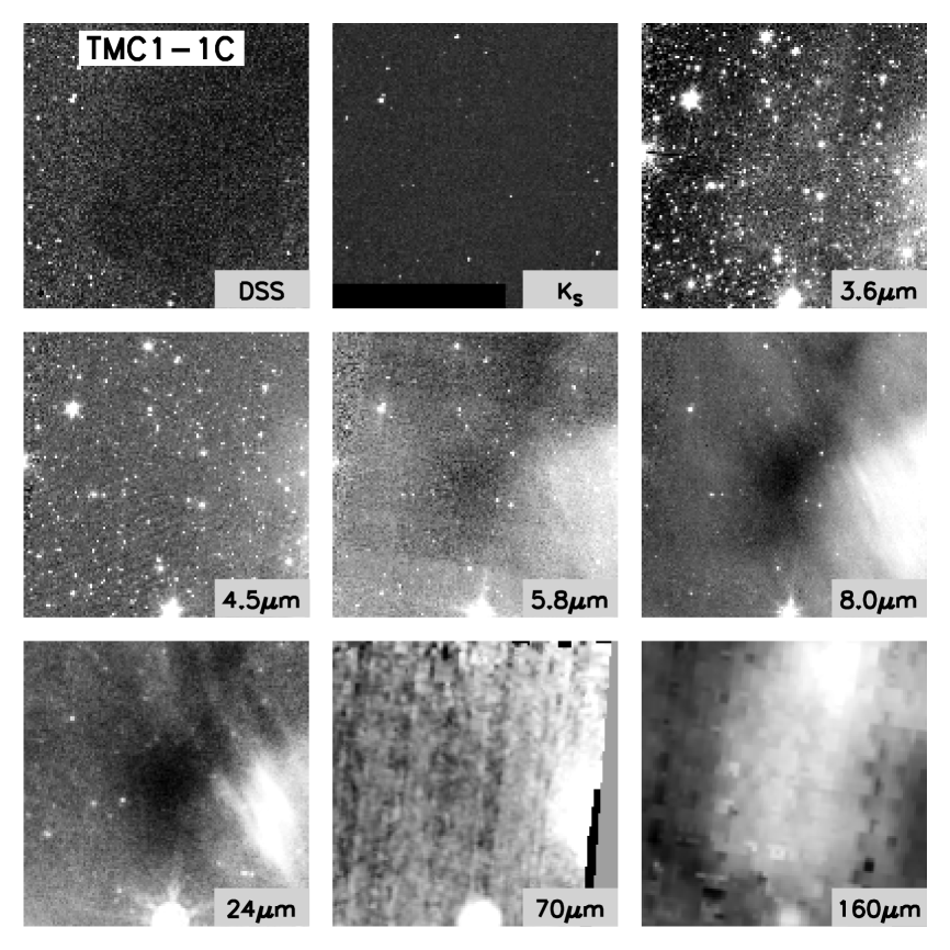
Figure 1.— $8\arcmin\times 8\arcmin$ images at the indicated wavelengths, shown on a log scale. North is up, east is to the left. For full resolution figures contact stutz@mpia.de.

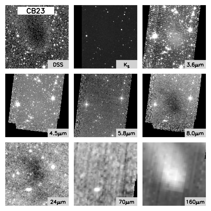
Figure 2.— Same as Figure 1

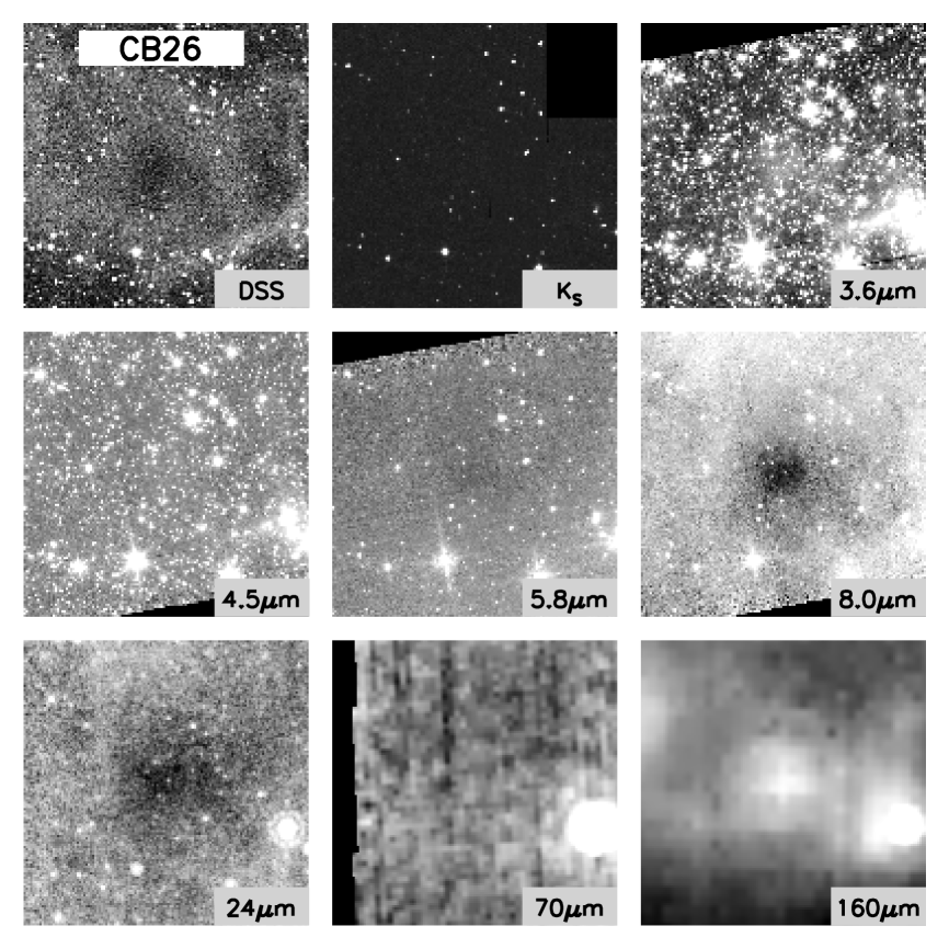
Figure 3.— Same as Figure 1

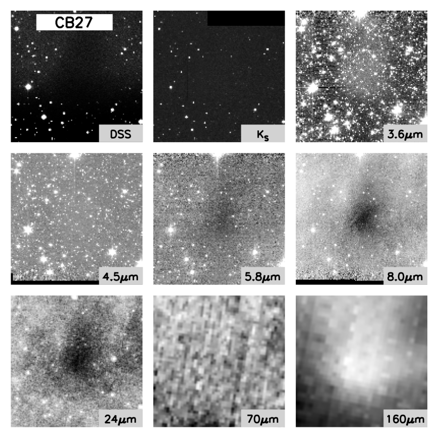
Figure 4.— Same as Figure 1

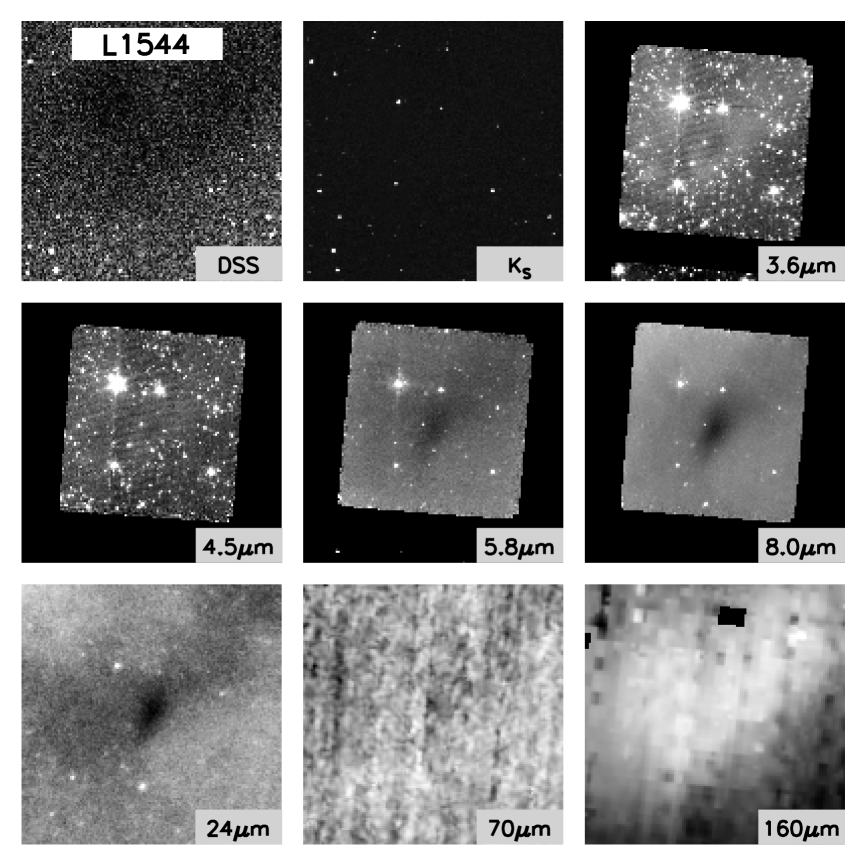
Figure 5.— Same as Figure 1

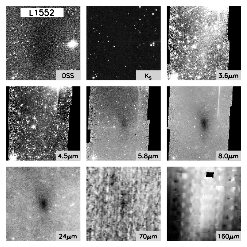
Figure 6.— Same as Figure 1

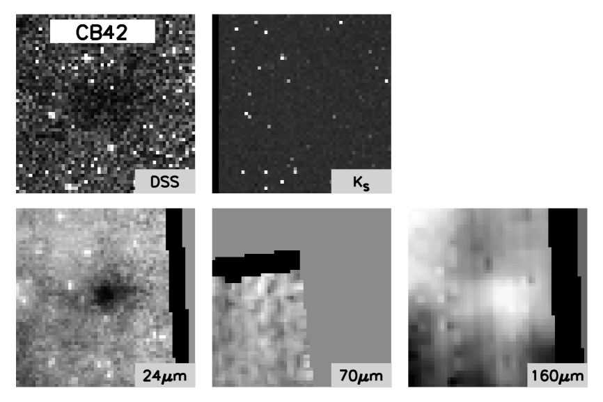
Figure 7.— Same as Figure 1

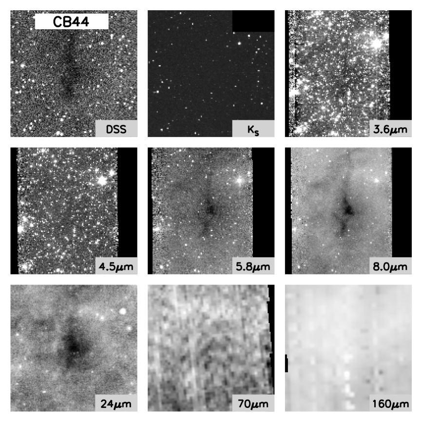
Figure 8.— Same as Figure 1

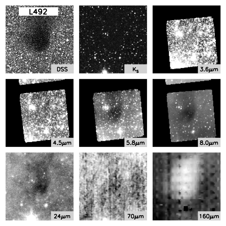
Figure 9.— Same as Figure 1

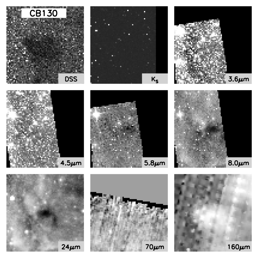
Figure 10.— Same as Figure 1

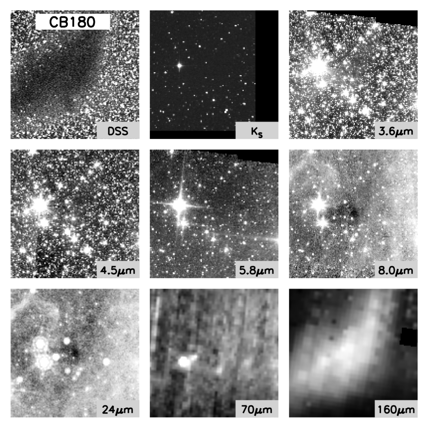
Figure 11.— Same as Figure 1

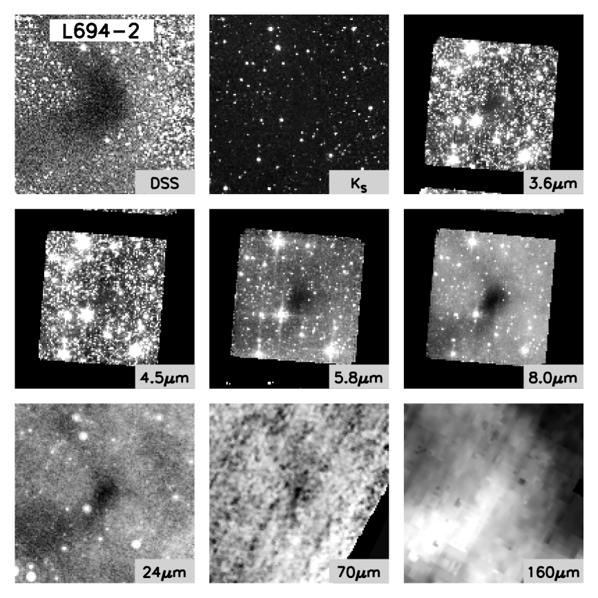
Figure 12.— Same as Figure 1

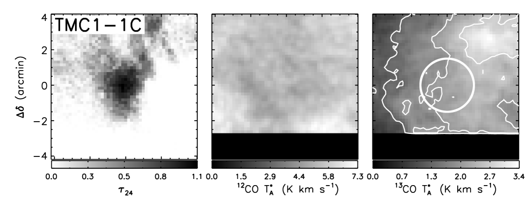
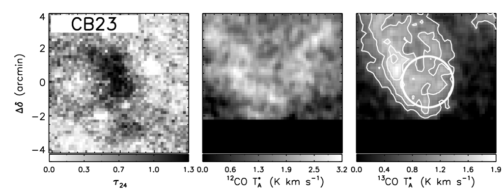
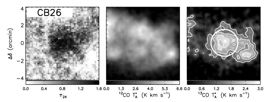
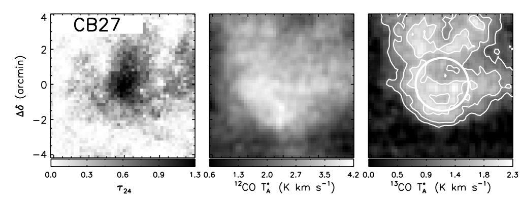
Figure 13.— $\tau_{24}$–maps and ¹²CO and ¹³CO integrated intensity maps, over the velocity ranges listed in Table 2. The black circle ($1\farcm 5$ radius) indicates the area used to calculate the 24 µm shadow masses; the white circle indicates that used to calculate the molecular masses. The ¹³CO contours levels are ${0.4,0.6,0.8}$ times the maximum value indicated int the ¹³CO color–bar. For full resolution figures contact stutz@mpia.de.

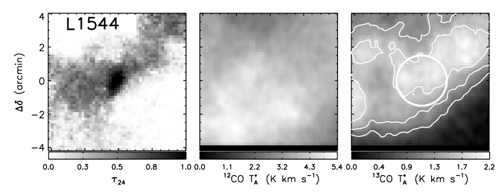
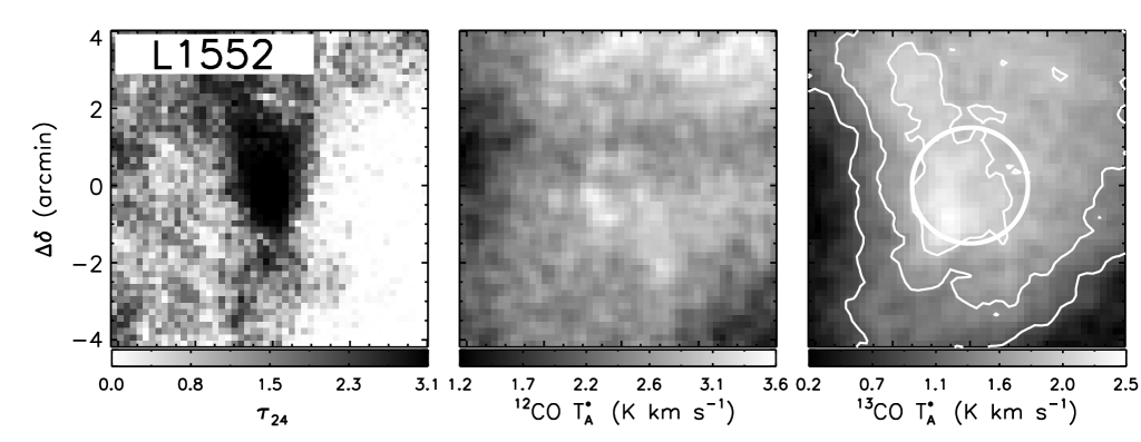
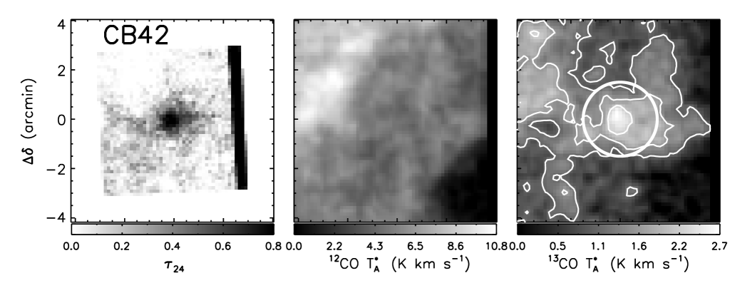
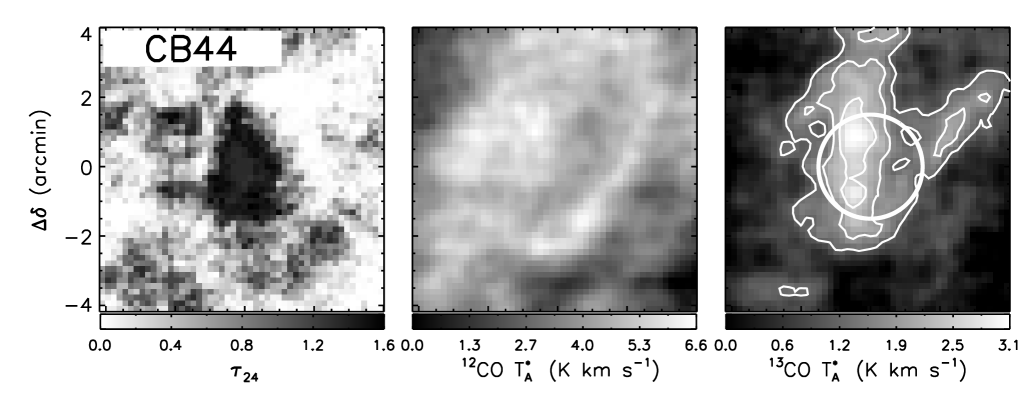
Figure 14.— Same as Figure 13

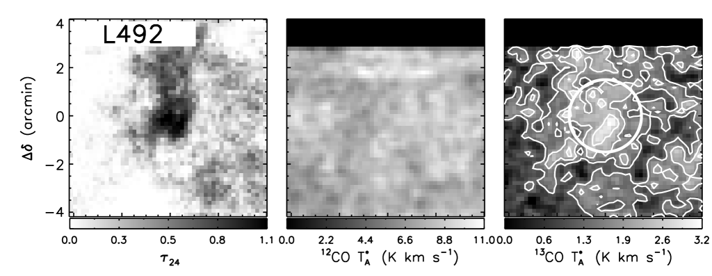
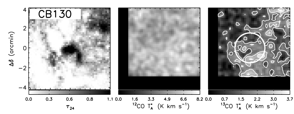
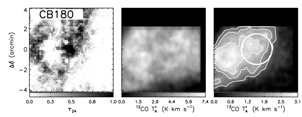
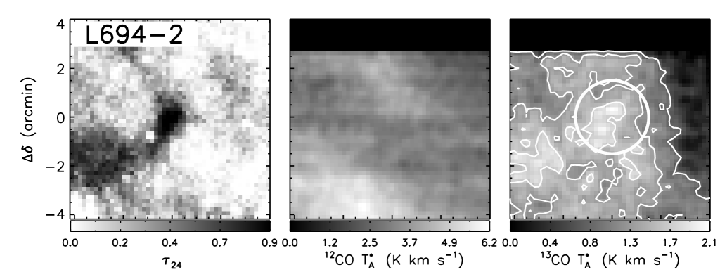
Figure 15.— Same as Figure 13

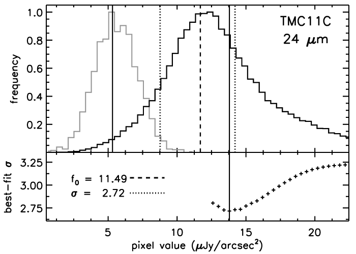
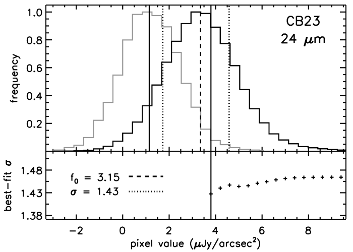
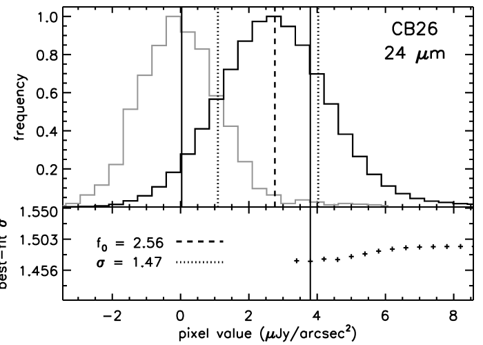
Figure 16.— Left Column, top panel — Black histogram: 24 µm pixel value distribution for background subtracted image region of $r_{0}=240\arcsec$ radius (except for CB42), $r_{0}$ is indicated in the right column as the dashed line, and is centered on the shadow. Grey histogram: 24 µm pixel value distribution for $30\arcsec$ region centered on the shadow. Solid lines: minimum and maximum black histogram bins used to fit for the minimum $\sigma$. The dashed line indicates the best–fit mean, or $f_{0}$, value at the minimum best–fit value for $\sigma$, indicated by the dotted line. Left Column, bottom panel — Best–fit values of $\sigma$ plotted against the maximum bin value included in the fit. The solid line indicates the minimum value of $\sigma$. Best–fit Gaussian parameters $\sigma$ and the mean ($f_{0}$) are indicated. Right Column: Best–fit $f_{0}$ and minimum $\sigma$ as a function of aperture size ($r_{0}$).

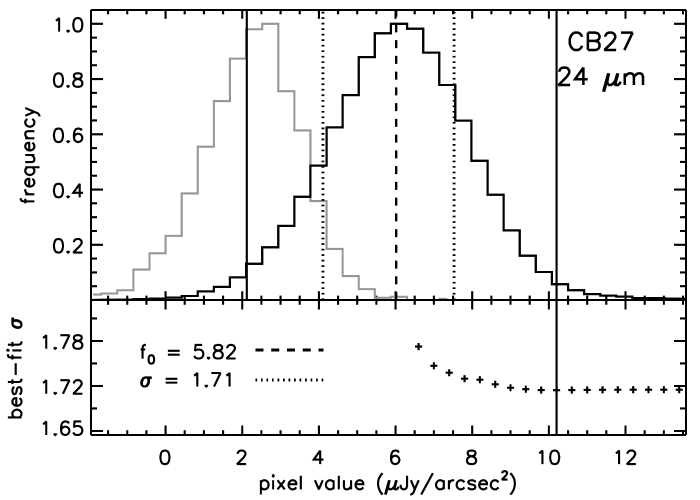
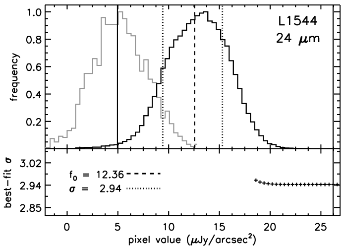
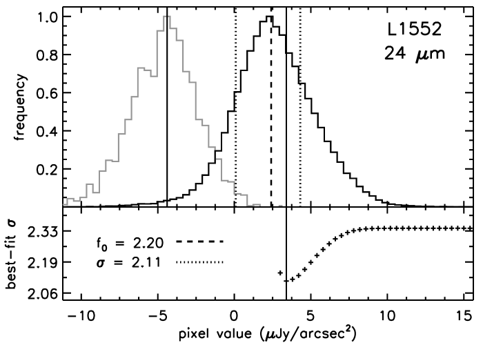
Figure 17.— Same as Figure 16

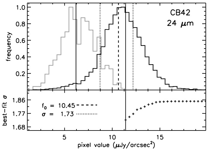
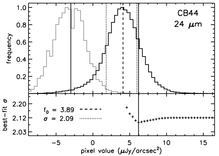
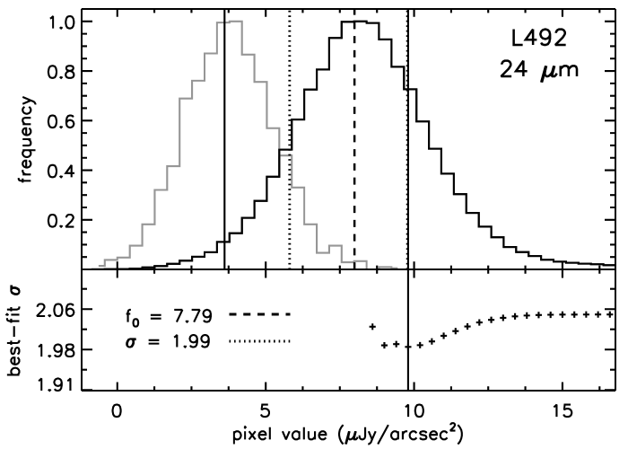
Figure 18.— Same as Figure 16

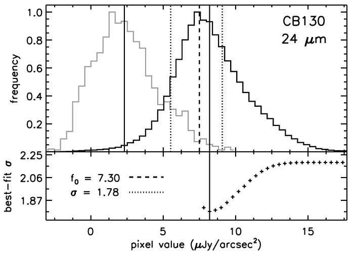
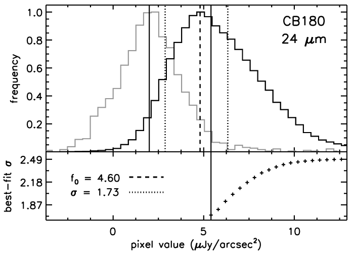
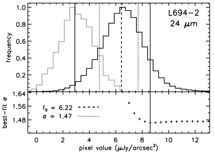
Figure 19.— Same as Figure 16

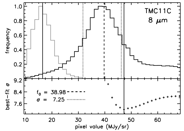
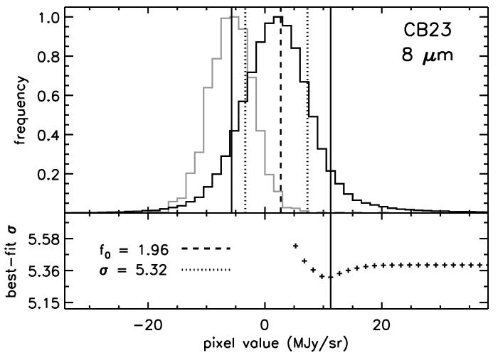
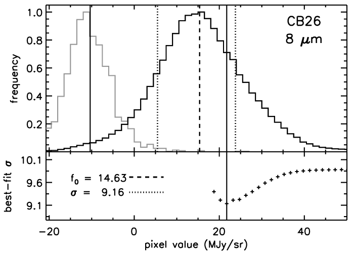
Figure 20.— Left Column, top panel — Black histogram: 8 µm pixel value distribution for background subtracted image region of $r_{0}=240\arcsec$ radius (except for CB42), $r_{0}$ is indicated in the right column as the dashed line, and is centered on the shadow. Grey histogram: 8 µm pixel value distribution for $30\arcsec$ region centered on the shadow. Solid lines: minimum and maximum black histogram bins used to fit for the minimum $\sigma$. The dashed line indicates the best–fit mean, or $f_{0}$, value at the minimum best–fit value for $\sigma$, indicated by the dotted line. Left Column, bottom panel — Best–fit values of $\sigma$ plotted against the maximum bin value included in the fit. The solid line indicates the minimum value of $\sigma$. Best–fit Gaussian parameters $\sigma$ and the mean ($f_{0}$) are indicated. Right Column — Best–fit $f_{0}$ and minimum $\sigma$ as a function of aperture size ( $r_{0}$).

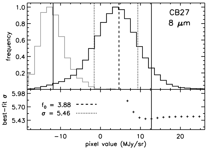
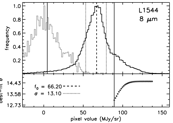
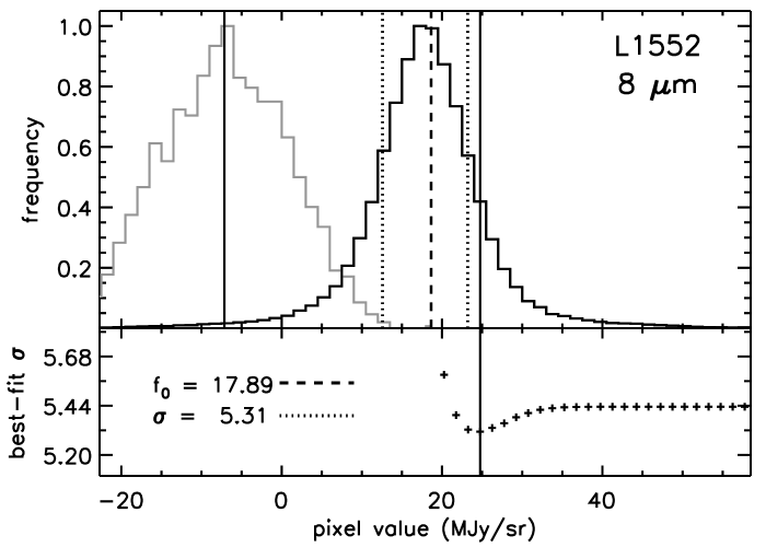
Figure 21.— Same as Figure 20

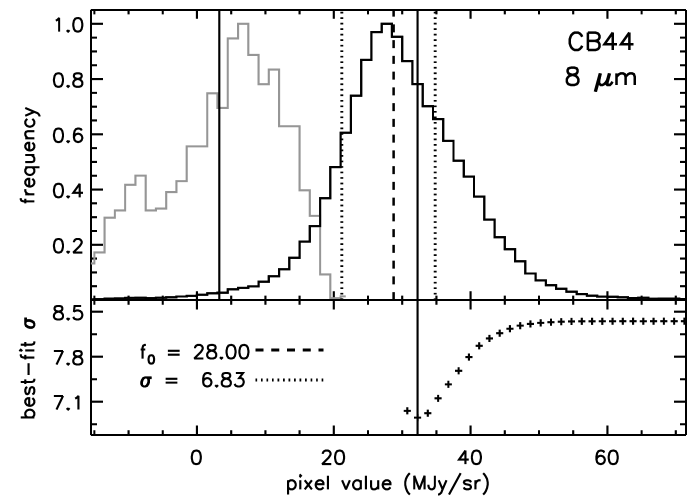
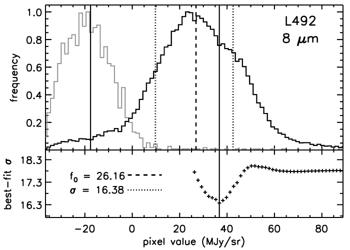
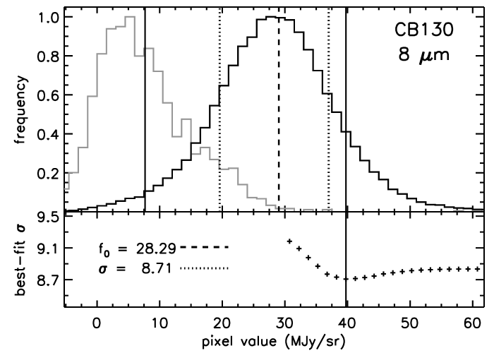
Figure 22.— Same as Figure 20

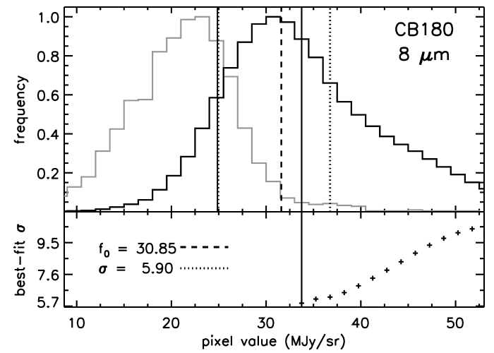
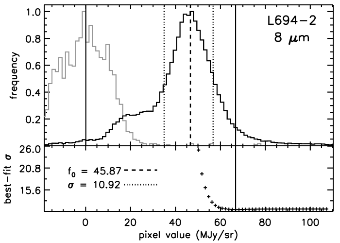
Figure 23.— Same as Figure 20

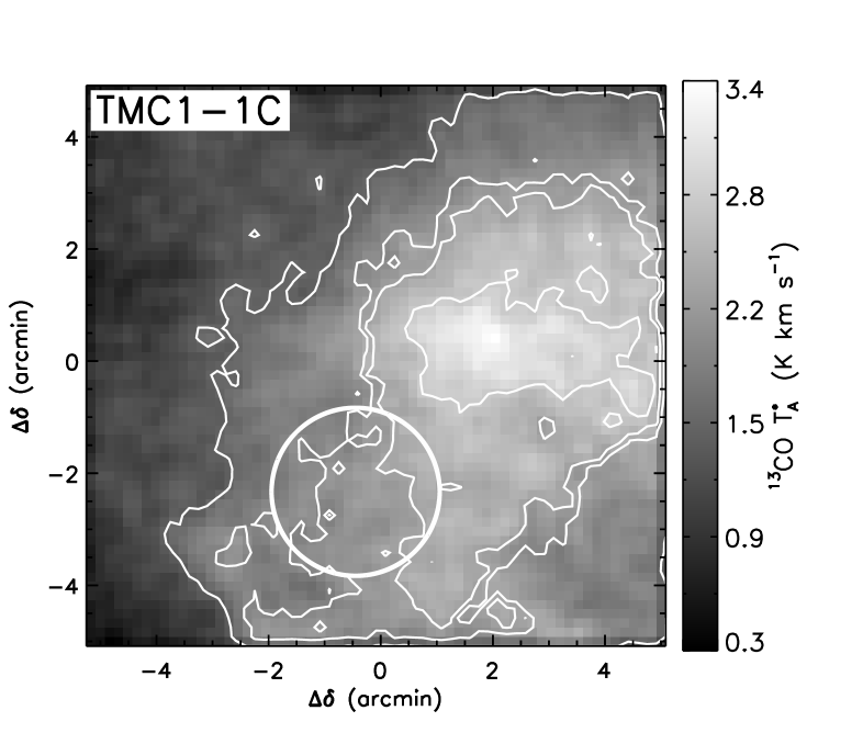
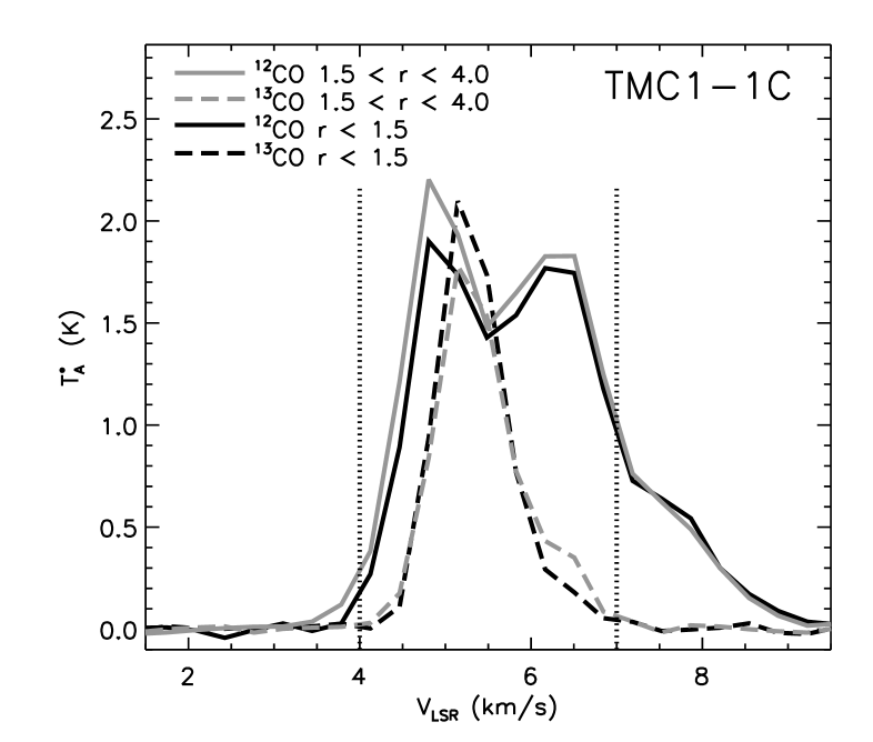
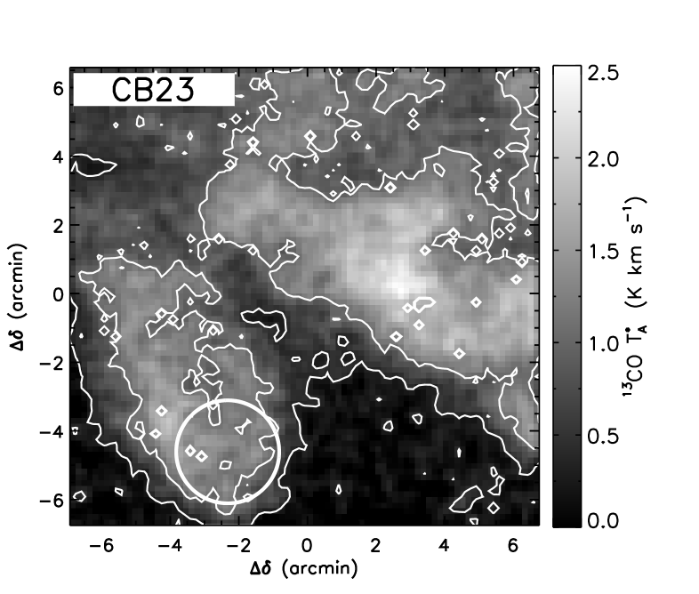
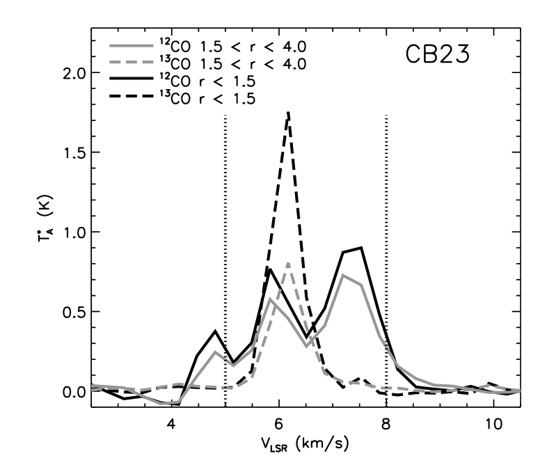
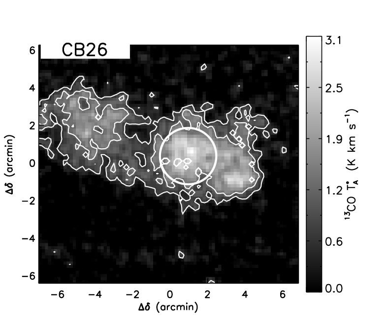
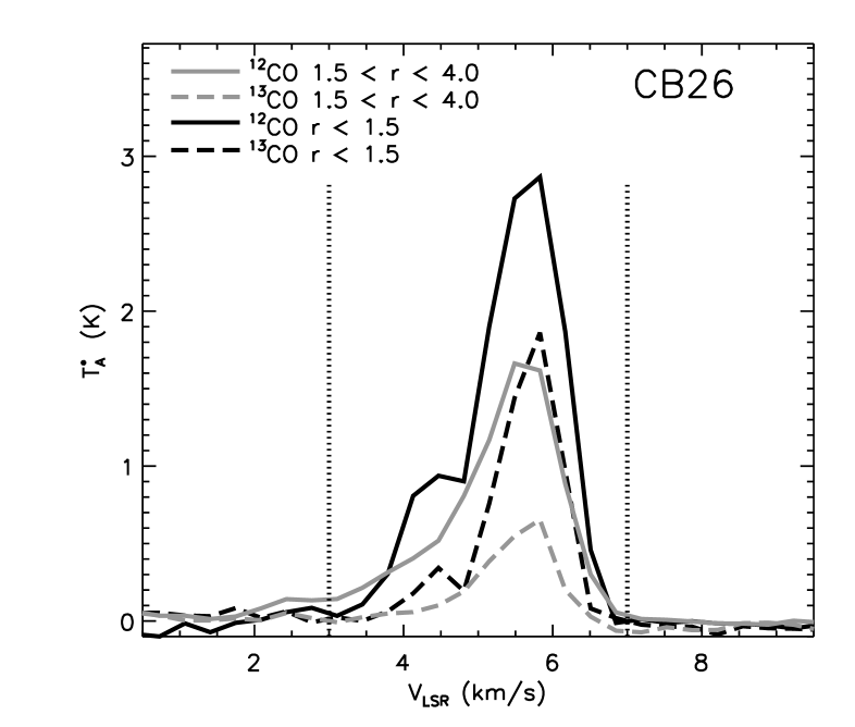
Figure 24.— Left Column — The grey scale image is ¹³CO (2-1) integrated intensity map. Contours are the CO–model derived N(H) column density maps, which show good spatial agreement between the molecular map; contour levels are scaled to the maximum value of the column density in the region of the shadow. Fractional contour levels for TMC-1C are $\{0.8,0.9,0.95,0.995\}\times 1.19\times 10^{22}$ cm^-2, for CB23 are $\{0.6,0.8\}\times 1.09\times 10^{22}$ cm^-2, and for CB26 are $\{0.5,0.6\}\times 1.49\times 10^{22}$ cm^-2. The shadow is indicated by the small white circle, with a radius of $1\farcm 5$; the large circle (r $=4\farcm 0$) indicates the region in which we calculate mass M_CO,4 (see Table 4 and text). Right Column — Mean ¹²CO and ¹³CO spectra for the regions indicated by the circles in the left panel. For full resolution figures contact stutz@mpia.de.

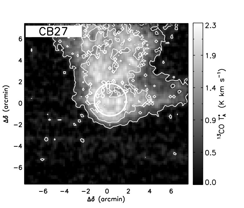
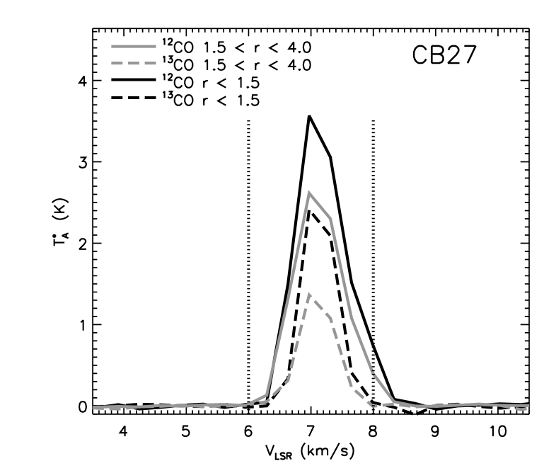
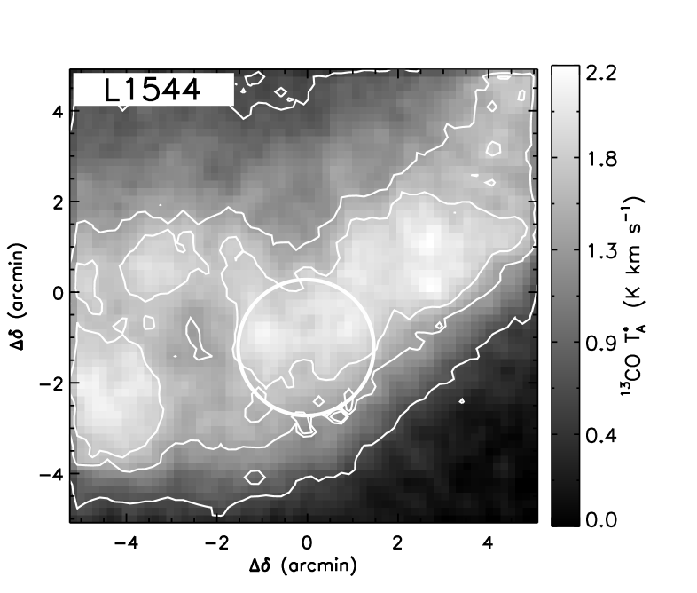
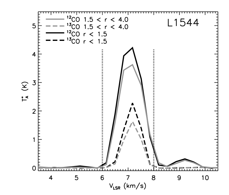
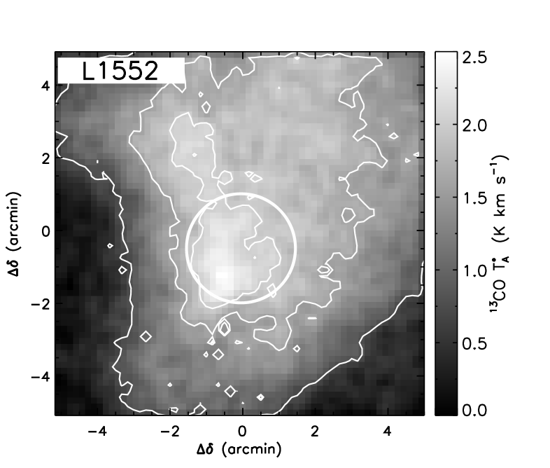
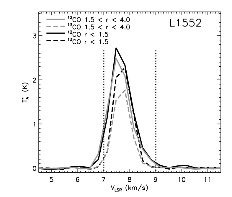
Figure 25.— Same as Figure 24. Fractional contour levels for CB27 are $\{0.5,0.7\}\times 1.40\times 10^{22}$ cm^-2, for L1544 are $\{0.7,0.9,0.95\}\times 1.11\times 10^{22}$ cm^-2, and L1552 are $\{0.7,0.9,0.95\}\times 1.15\times 10^{22}$ cm^-2.

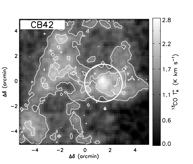
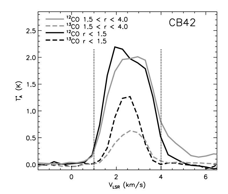
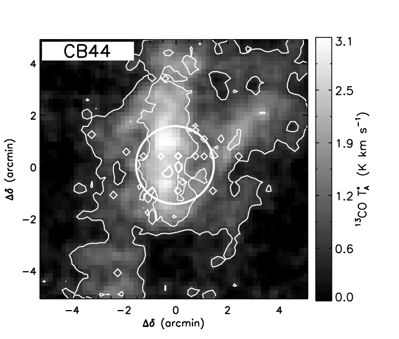
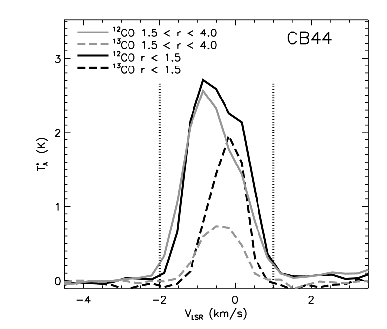
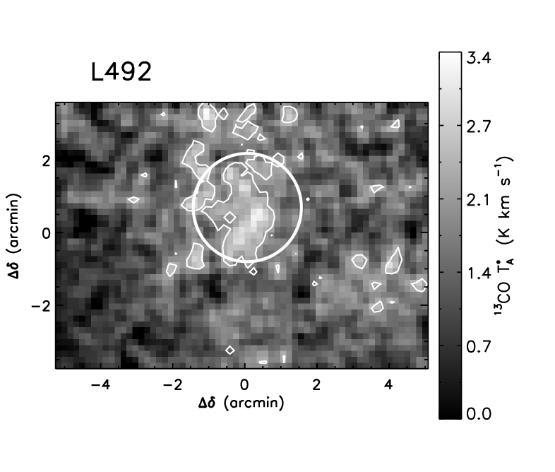
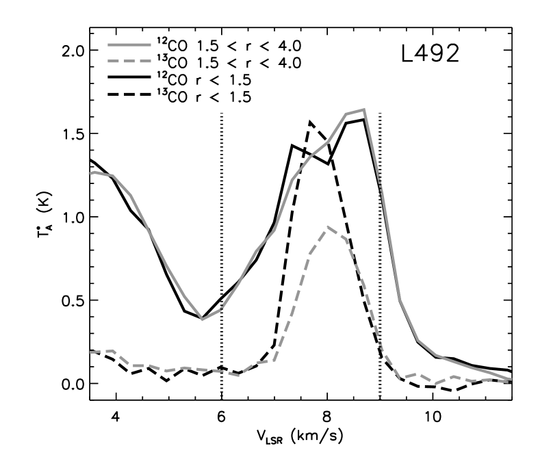
Figure 26.— Same as Figure 24. Fractional contour levels for CB42 are $\{0.75,0.85\}\times 1.19\times 10^{22}$ cm^-2, for CB44 are $\{0.4,0.55\}\times 1.86\times 10^{22}$ cm^-2, and L492 are $\{0.85\}\times 1.24\times 10^{22}$ cm^-2.

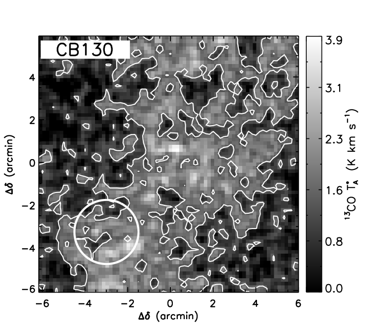
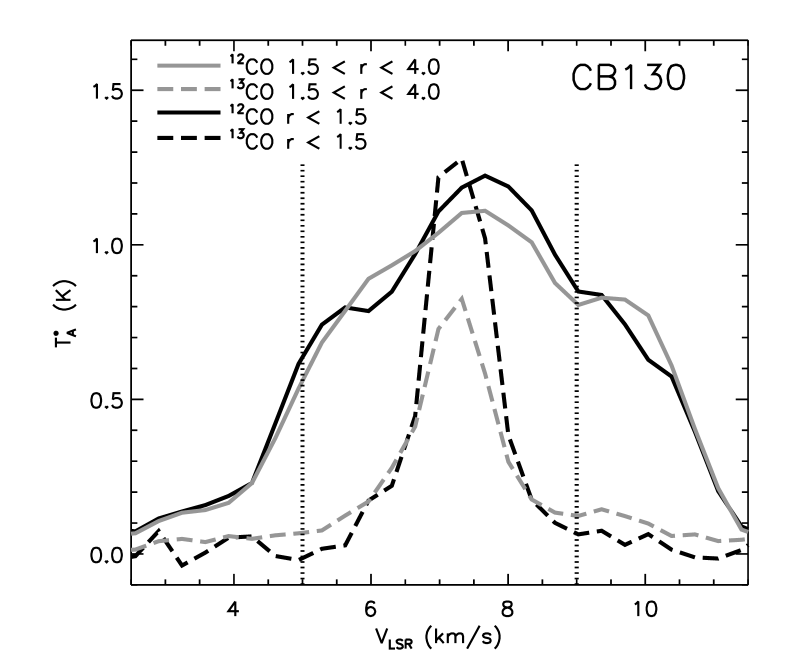
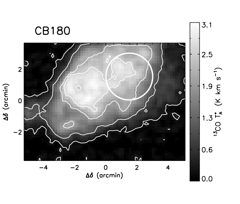
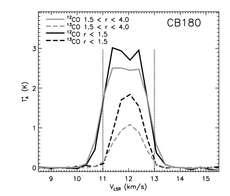
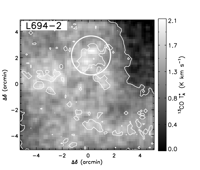
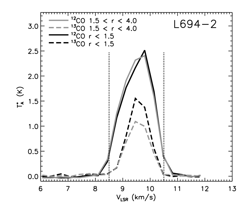
Figure 27.— Same as Figure 24. Fractional contour levels for CB130 are $\{0.75\}\times 1.21\times 10^{22}$ cm^-2, for CB180 are $\{0.5,0.7,0.9,0.97\}\times 1.21\times 10^{22}$ cm^-2, and L694-2 are $\{0.7,0.9\}\times 1.11\times 10^{22}$ cm^-2.

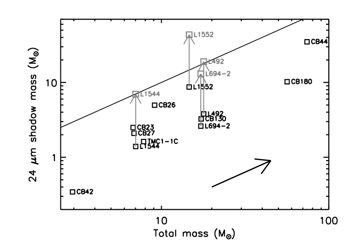
Figure 28.— Masses presented Table 4 are plotted here. Top panel — The CO core masses calculated over the area of the core are plotted versus the 24 µm shadow masses. Bottom panel — The total masses (M_CO,4 $+$ M${}_{24}^{\rm core}$ $-$ M${}_{\rm CO}^{\rm core}$) are plotted versus the 24 µm shadow masses. The arrow indicates the effect of 50% change in the assumed distance. In both panels the black curve indicates equality between the ordinate and the abscissa.

References

- Alves et al. (2001) Alves, J. F., Lada, C. J., & Lada, E. A. 2001, Nature, 409, 159
- Alves et al. (2008) Alves, F. O., Franco, G. A. P., & Girart, J. M. 2008, A&A, 486, L13
- Arquilla & Goldsmith (1986) Arquilla, R., & Goldsmith, P. F. 1986, ApJ, 303, 356
- Bacmann et al. (2000) Bacmann, A., André, P., Puget, J.-L., Abergel, A., Bontemps, S., & Ward-Thompson, D. 2000, A&A, 361, 555
- Bacmann et al. (2002) Bacmann, A., Lefloch, B., Ceccarelli, C., Castets, A., Steinacker, J., & Loinard, L. 2002, A&A, 389, L6
- Bacmann et al. (2003) Bacmann, A., Lefloch, B., Ceccarelli, C., Steinacker, J., Castets, A., & Loinard, L. 2003, ApJ, 585, L55
- Ballesteros-Paredes et al. (2003) Ballesteros-Paredes, J., Klessen, R. S., & Vázquez-Semadeni, E. 2003, ApJ, 592, 188
- Bergin & Tafalla (2007) Bergin, E. A., & Tafalla, M. 2007, ARA&A, 45, 339
- Bok & McCarthy (1974) Bok, B. J., & McCarthy, C. C. 1974, AJ, 79, 42
- Burkert & Bodenheimer (2000) Burkert, A., & Bodenheimer, P. 2000, ApJ, 543, 822
- Burkert & Hartmann (2004) Burkert, A., & Hartmann, L. 2004, ApJ, 616, 288
- Butler & Tan (2009) Butler, M. J., & Tan, J. C. 2009, ApJ, 696, 484
- Caselli et al. (1999) Caselli, P., Walmsley, C. M., Tafalla, M., Dore, L., & Myers, P. C. 1999, ApJ, 523, L165
- Caselli et al. (2002) Caselli, P., Benson, P. J., Myers, P. C., & Tafalla, M. 2002, ApJ, 572, 238
- Caselli et al. (2008) Caselli, P., Vastel, C., Ceccarelli, C., van der Tak, F. F. S., Crapsi, A., & Bacmann, A. 2008, A&A, 492, 703
- Chapman et al. (2009) Chapman, N. L., Mundy, L. G., Lai, S.-P., & Evans, N. J. 2009, ApJ, 690, 496
- Chapman & Mundy (2009) Chapman, N. L., & Mundy, L. G. 2009, arXiv:0905.0655
- Clemens & Barvainis (1988) Clemens, D. P., & Barvainis, R. 1988, ApJS, 68, 257
- Crapsi et al. (2005) Crapsi, A., Caselli, P., Walmsley, C. M., Myers, P. C., Tafalla, M., Lee, C. W., & Bourke, T. L. 2005, ApJ, 619, 379
- de Wit et al. (2005) de Wit, W. J., Testi, L., Palla, F., & Zinnecker, H. 2005, A&A, 437, 247
- Draine (2003) Draine, B. T. 2003, ARA&A, 41, 241
- Evans et al. (2001) Evans, N. J., Rawlings, J. M. C., Shirley, Y. L., & Mundy, L. G. 2001, ApJ, 557, 193
- Fallscheer et al. (2009) Fallscheer, C., Beuther, H., Zhang, Q., Keto, E., & Sridharan, T. K. 2009, arXiv:0907.2232
- Flaherty et al. (2007) Flaherty, K. M., Pipher, J. L., Megeath, S. T., Winston, E. M., Gutermuth, R. A., Muzerolle, J., Allen, L. E., & Fazio, G. G. 2007, ApJ, 663, 1069
- Foster & Goodman (2006) Foster, J. B., & Goodman, A. A. 2006, ApJ, 636, L105
- Gregersen et al. (1997) Gregersen, E. M., Evans, N. J., II, Zhou, S., & Choi, M. 1997, ApJ, 484, 256
- Gregersen & Evans (2000) Gregersen, E. M., & Evans, N. J., II 2000, ApJ, 538, 260
- Gordon et al. (2005) Gordon, K. D., et al. 2005, PASP, 117, 503
- Gupta et al. (2009) Gupta, H., Gottlieb, C. A., McCarthy, M. C., & Thaddeus, P. 2009, ApJ, 691, 1494
- Gutermuth et al. (2008) Gutermuth, R. A., et al. 2008, ApJ, 674, 336
- Harvey et al. (2003a) Harvey, D. W. A., Wilner, D. J., Lada, C. J., Myers, P. C., & Alves, J. F. 2003a, ApJ, 598, 1112
- Harvey et al. (2003b) Harvey, D. W. A., Wilner, D. J., Myers, P. C., & Tafalla, M. 2003b, ApJ, 597, 424
- Hayashi (1966) Hayashi, C. 1966, ARA&A, 4, 171
- Heitsch et al. (2008) Heitsch, F., Hartmann, L. W., Slyz, A. D., Devriendt, J. E. G., & Burkert, A. 2008, ApJ, 674, 316
- Henning et al. (2001) Henning, T., Wolf, S., Launhardt, R., & Waters, R. 2001, ApJ, 561, 871
- Hilton & Lahulla (1995) Hilton, J., & Lahulla, J. F. 1995, A&AS, 113, 325
- Hotzel et al. (2002) Hotzel, S., Harju, J., & Juvela, M. 2002, A&A, 395, L5
- Juvela et al. (2008) Juvela, M., Pelkonen, V.-M., Padoan, P., & Mattila, K. 2008, A&A, 480, 445
- Kandori et al. (2005) Kandori, R., et al. 2005, AJ, 130, 2166
- Kang et al. (2009) Kang, M., Bieging, J. H., Kulesa, C. A., & Lee, Y. 2009, ApJ, 701, 454
- Kauffmann et al. (2008) Kauffmann, J., Bertoldi, F., Bourke, T. L., Evans, N. J., II, & Lee, C. W. 2008, A&A, 487, 993
- Kawamura et al. (2001) Kawamura, A., Kun, M., Onishi, T., Vavrek, R., Domsa, I., Mizuno, A., & Fukui, Y. 2001, PASJ, 53, 1097
- Kenyon et al. (1994) Kenyon, S. J., Dobrzycka, D., & Hartmann, L. 1994, AJ, 108, 1872
- Kulesa et al. (2005) Kulesa, C. A., Hungerford, A. L., Walker, C. K., Zhang, X., & Lane, A. P. 2005, ApJ, 625, 194
- Kutner & Ulich (1981) Kutner, M. L., & Ulich, B. L. 1981, ApJ, 250, 341
- Lada & Lada (2003) Lada, C. J., & Lada, E. A. 2003, ARA&A, 41, 57
- Lada et al. (2008) Lada, C. J., Muench, A. A., Rathborne, J., Alves, J. F., & Lombardi, M. 2008, ApJ, 672, 410
- Lallement et al. (2003) Lallement, R., Welsh, B. Y., Vergely, J. L., Crifo, F., & Sfeir, D. 2003, A&A, 411, 447
- Launhardt et al. (1998) Launhardt, R., Evans, N. J., II, Wang, Y., Clemens, D. P., Henning, T., & Yun, J. L. 1998, ApJS, 119, 59
- Launhardt et al. (2009) Launhardt, R., et al. 2009, A&A, 494, 147
- Lee et al. (1999) Lee, C. W., Myers, P. C., & Tafalla, M. 1999, ApJ, 526, 788
- Lee et al. (2003) Lee, J.-E., Evans, N. J., II, Shirley, Y. L., & Tatematsu, K. 2003, ApJ, 583, 789
- Lee et al. (2004) Lee, C. W., Myers, P. C., & Plume, R. 2004, ApJS, 153, 523
- Lee et al. (2007) Lee, S. H., Park, Y.-S., Sohn, J., Lee, C. W., & Lee, H. M. 2007, ApJ, 660, 1326
- Lee et al. (2009) Lee, M.-Y., et al. 2009, arXiv:0908.2275
- Lehtinen & Mattila (1996) Lehtinen, K., & Mattila, K. 1996, A&A, 309, 570
- Lemme et al. (1996) Lemme, C., Wilson, T. L., Tieftrunk, A. R., & Henkel, C. 1996, A&A, 312, 585
- Mardones et al. (1997) Mardones, D., Myers, P. C., Tafalla, M., Wilner, D. J., Bachiller, R., & Garay, G. 1997, ApJ, 489, 719
- Menten et al. (1987) Menten, K. M., Serabyn, E., Guesten, R., & Wilson, T. L. 1987, A&A, 177, L57
- Mundy et al. (1990) Mundy, L. G., Wootten, H. A., & Wilking, B. A. 1990, ApJ, 352, 159
- Myers (2005) Myers, P. C. 2005, ApJ, 623, 280
- Nakajima et al. (2008) Nakajima, Y., Kandori, R., Tamura, M., Nagata, T., Sato, S., & Sugitani, K. 2008, PASJ, 60, 731
- Narayanan et al. (1998) Narayanan, G., Walker, C. K., & Buckley, H. D. 1998, ApJ, 496, 292
- Ossenkopf & Henning (1994) Ossenkopf, V., & Henning, T. 1994, A&A, 291, 943
- Padoan et al. (2006) Padoan, P., Juvela, M., & Pelkonen, V.-M. 2006, ApJ, 636, L101
- Park et al. (2004) Park, Y.-S., Lee, C. W., & Myers, P. C. 2004, ApJS, 152, 81
- Perault et al. (1996) Perault, M., et al. 1996, A&A, 315, L165
- Peretto & Fuller (2009) Peretto, N., & Fuller, G. A. 2009, arXiv:0906.3493
- Povich et al. (2009) Povich, M. S., et al. 2009, ApJ, 696, 1278
- Roberts & Millar (2007) Roberts, H., & Millar, T. J. 2007, A&A, 471, 849
- Sault et al. (1995) Sault R.J., Teuben P.J., Wright M.C.H., 1995, in Astronomical Data Analysis Software and Systems IV, ed. R. Shaw, H.E. Payne, J.J.E. Hayes, ASP Conf. Ser., 77, 433-436
- Sauter et al. (2009) Sauter, J., et al. 2009, arXiv:0907.1074
- Shirley et al. (2000) Shirley, Y. L., Evans, N. J., II, Rawlings, J. M. C., & Gregersen, E. M. 2000, ApJS, 131, 249
- Shirley et al. (2005) Shirley, Y. L., Nordhaus, M. K., Grcevich, J. M., Evans, N. J., Rawlings, J. M. C., & Tatematsu, K. 2005, ApJ, 632
- Shu et al. (1987) Shu, F. H., Adams, F. C., & Lizano, S. 1987, ARA&A, 25, 23
- Sohn et al. (2007) Sohn, J., Lee, C. W., Park, Y.-S., Lee, H. M., Myers, P. C., & Lee, Y. 2007, ApJ, 664, 928
- Stahler & Palla (2005) Stahler, S. W., & Palla, F. 2005, The Formation of Stars, by Steven W. Stahler, Francesco Palla, pp. 865. ISBN 3-527-40559-3. Wiley-VCH , January 2005.
- Straižys et al. (2003) Straižys, V., Černis, K., & Bartašiūtė, S. 2003, A&A, 405, 585
- Stecklum et al. (2004) Stecklum, B., Launhardt, R., Fischer, O., Henden, A., Leinert, C., & Meusinger, H. 2004, ApJ, 617, 418
- Stutz et al. (2007) Stutz, A. M., et al. 2007, ApJ, 665, 466
- Stutz et al. (2008a) Stutz, A. M., Papovich, C., & Eisenstein, D. J. 2008a, ApJ, 677, 828
- Stutz et al. (2008b) Stutz, A. M., et al. 2008b, ApJ, 687, 389
- Stutz et al. (2009) Stutz, A. M., Bourke, T. L., Rieke, G. H., Bieging, J. H., Misselt, K. A., Myers, P. C., & Shirley, Y. L. 2009, ApJ, 690, L35
- Tafalla et al. (2002) Tafalla, M., Myers, P. C., Caselli, P., Walmsley, C. M., & Comito, C. 2002, ApJ, 569, 815
- Tomita et al. (1979) Tomita, Y., Saito, T., & Ohtani, H. 1979, PASJ, 31, 407
- Torres et al. (2009) Torres, R. M., Loinard, L., Mioduszewski, A. J., & Rodriguez, L. F. 2009, arXiv:0903.5338
- Turner et al. (1997) Turner, B. E., Pirogov, L., & Minh, Y. C. 1997, ApJ, 483, 235
- van Dishoeck & Black (1988) van Dishoeck, E. F., & Black, J. H. 1988, ApJ, 334, 771
- Walker et al. (1986) Walker, C. K., Lada, C. J., Young, E. T., Maloney, P. R., & Wilking, B. A. 1986, ApJ, 309, L47
- Walker et al. (1988) Walker, C. K., Lada, C. J., Young, E. T., & Margulis, M. 1988, ApJ, 332, 335
- Williams et al. (2006) Williams, J. P., Lee, C. W., & Myers, P. C. 2006, ApJ, 636, 952