Frictional Drag induced in Low- Dimensional Systems by Brownian Motion of Ions in Liquid Flow

Abstract

We study the frictional drag force in low-dimensional systems (2D-electron and 2D-liquid systems) mediated by a fluctuating electromagnetic field which originate from Brownian motion of ions in liquid. The analysis is focused on the [2D-system–2D-system], [2D-system –semi-infinite liquid], and [2D-system–infinite liquid] configurations. We show that for 2D-electron systems the friction drag depends linearly on the relative velocity of the free carries of charge in the different media, but for 2D-liquid systems the frictional drag depends nonlinear on the relative velocity. For 2D-systems the frictional drag force induced by liquid flow may be several orders of magnitude larger than the frictional drag induced by an electronic current.

PACS: 47.61.-k, 44.40.+a, 68.35.Af

I Introduction

All media are surrounded by a fluctuating electromagnetic field because of the thermal and quantum fluctuations of the current density inside them. The fluctuating field is responsible for many important phenomena such as radiative heat transfer, the van der Waals interaction, noncontact friction and frictional drag in low-dimensional systems Greffet6 ; RMP07 . The relation between fluctuations and friction is determined by the fluctuation-dissipation theorem. According to this theorem, the fluctuating force that makes a small particle jitter will also cause friction if the particle is dragged through the medium. Noncontact friction and frictional drag measurements are very closely related to each other. In both these experiments the media are separated by a potential barrier thick enough to prevent electrons or other particle with a finite rest mass from tunneling across it, but allowing the interaction via the long-range electromagnetic field, which is always present in the gap between bodies. In noncontact friction experiments the bodies move relative to each other, while in frictional drag experiments the motion of charged particles (electrons or ions) is induced in one medium, and the reaction of free carries of charge on this motion is measured in other medium (see Fig. 1)

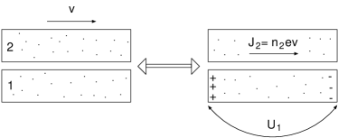
Figure 1: Two way for studying noncontact friction. Left: Two bodies at finite separation are sliding relative to each other. The noncontact friction force between bodies is mediated by a fluctuating electromagnetic field. Right: A current of charged particles (electrons or ions) flow in upper medium. The fluctuating electromagnetic field associated with this motion will result in friction force acting on the free electrons or ions in medium at the bottom. This friction force will induce an electric field which can be measured.

There are two mechanisms of noncontact friction and frictional drag. The electrostatic friction is due to the relative motion of charged bodies. This mechanism of noncontact friction was observed in Stipe ; Kuehn2006 . In these experiments a charged probe tip oscillated close to the surface of substrate. Measurement of the damping of the probe oscillation yields a noncontact friction coefficient that may be related to the spectrum of the electromagnetic field fluctuation at the probe frequency. Using the fluctuation-dissipation theorem, the force fluctuations were interpreted Stipe ; Kuehn2006 in terms of near-surface fluctuating electric field interacting with static surface charge. The electrostatic friction can be related to the ‘image’ charge which is induced in the sample by the charged tip. During motion of the tip relative to the sample the “image” charge will lag slightly behind the moving charge inducing it, and this is the origin of the electrostatic friction Volokitin2005 ; Volokitin2006 .

Noncontact friction exists even between neutral bodies because the fluctuating electromagnetic field originated from charge fluctuations in one medium will induce polarization in other medium. The interaction of the fluctuating electromagnetic field with the induced polarization is responsible for many important phenomena such as radiative heat transfer and the van der Waals interaction RMP07 . When two media are in relative motion, the induced polarization will lag behind the fluctuating polarization inducing it, and this gives rise to the so-called van der Waals friction.

The origin of the van der Waals friction is closely connected with the Doppler effect. Let us consider two flat parallel surfaces, separated by a sufficiently wide insulator gap, which prevents particles from tunneling across it. If the charge carriers inside the volumes restricted by these surfaces are in relative motion (velocity $v$) a frictional stress will act between surfaces. This frictional stress is related to an asymmetry of the reflection amplitude along the direction of motion; see Fig. 2.

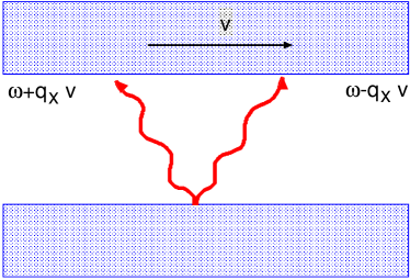
Figure 2: Two bodies moving relative to each other will experience van der Waals friction due to Doppler shift of the electromagnetic waves emitted by them.

If one body emits radiation, then in the rest reference frame of the second body these waves are Doppler shifted which will result in different reflection amplitudes. The same is true for radiation emitted by the second body. The exchange of “Doppler-shifted-photons” will result in momentum transfer between bodies which is the origin of the van der Waals friction.

The van der Waals friction can be probed not only by measuring the friction force during relative motion of the two bodies, but an alternative method consists in driving an electric current in one metallic layer and studying of the effect of the frictional drag of the electrons in a second (parallel) metallic layer (Fig. 3).

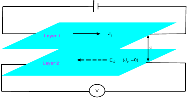
Figure 3: A schematic diagram of a drag experiment. A current $\mathbf{J_{1}}$ is passed through layer 1, and a voltmeter is attached to layer 2 to measure the induced electric field $\mathbf{E_{2}}$ due to interlayer interaction.

Such experiments were suggested by Pogrebinskii Pogrebinskii and Price Price , and were performed for 2D-quantum wells Gramila1 ; Sivan . In these experiments, two quantum wells are separated by a dielectric layer thick enough to prevent electrons from tunneling across it but allowing interlayer interaction between them. A current of density $J_{1}=n_{1}ev$ is driven through layer 1 (where $n_{`}$ is the carrier concentration per unit area in the first layer), see Fig. 3. Due to the interlayer interactions a frictional stress $\sigma=\gamma v$ will act on the electrons in the layer 2 from layer 1 which will induce a current in layer 2. If layer 2 is an open circuit, an electric field $E_{2}$ will develop in the layer whose influence cancels the frictional stress $\sigma$ between the layers. Experiments Gramila1 show that, at least for small separations, the frictional drag can be explained by the interaction between the electrons in the different layers via the fluctuating Coulomb field. However, for large inter-layer separation the friction drag is dominated by phonon exchange Bonsager .

Recently, it was observed that the flow of a liquid over bundles of single-walled carbon nanotubes (SWNT) induces a voltage in the sample along the direction of the flow Kumar1 ; Kumar2 . The dependence of the voltage on the flow speed was found to be logarithmic over five decades of variation of the speed. There have been attempts to explain this flow-induced voltage in electrokinetic terms, as a result of the streaming potential that develops along the flow of an electrolyte through a microporous insulator Cohen ; Ghosh . Earlier Král and Shapiro Kral proposed that the liquid flow transfer momentum to the acoustic phonons of the nanotube, and that the resulting “phonon wind” drives an electric current in the nanotube. They also suggested, qualitatively, that the fluctuating Coulomb field of the ions in the liquid could drag directly the carriers in the nanotube. However, the first mechanism Kral requires an enormous pressure Kumar2 , while the second mechanism Kral result in a very small current, of order femtoAmperes Kumar2 . In Kumar2 another mechanism was proposed, which is related to the second idea of Ref. Kral , but which requires neither localization of carriers nor drag at the same speed as the ions. In fact, Kumar2 considered the friction between a moving point charge and the surrounding medium. This mechanism of friction is described by the theory of electrostatic friction RMP07 . For neutral systems, such as a nanotube, the electrostatic friction proposed in Kumar2 will vanishing.

In Persson7 it was assumed that the liquid molecules nearest to the nanotube form a 2D-solidlike monolayer, pinned to the nanotube by adsorbed ions. As the liquid flows, the adsorbed solid monolayer performs stick-slip type of sliding motion along the nanotube. The drifting adsorbed ions will produce a voltage in the nanotube through electronic friction against free electrons inside the nanotube.

In Das a model calculations of the frictional drag were presented involving a channel containing overdamped Brownian particles. The channel was embedded in a wide chamber containing the same type of Brownian particles with drift velocity parallel to the channel. It was found that the flow of particles in the chamber induces a drift of the particles in the channel.

In this article we study frictional drag in low-dimensional system mediated by the fluctuating electromagnetic field originated from Brownian motion of ions. We compare this mechanism of frictional drag with the frictional drag resulting from charge fluctuations in electron system. A Brief Report about this work was published in Volokitin08 .

II van der Waals frictional drag between two 2D-systems

Let us consider two media with flat parallel surfaces at separation $d\ll\lambda_{T}=c\hbar/k_{B}T$. Assume that the free charge carriers in one media move with the velocity $v$ relative to other medium. According to Volokitin6 ; Volokitin10 the frictional stress between the two media, mediated by a fluctuating electromagnetic field, is determined by

$$\sigma_{\|}=\frac{\hbar}{2\pi^{3}}\int_{-\infty}^{\infty}dq_{y}\int_{0}^{\infty}dq_{x}q_{x}e^{-2qd}\left\{\int_{0}^{\infty}d\omega[n(\omega)-n(\omega+q_{x}v)]\right.$$

$$\times\left(\frac{\mathrm{Im}R_{1p}(\omega+q_{x}v)\mathrm{Im}R_{2p}(\omega)}{\mid 1-e^{-2qd}R_{1p}(\omega+q_{x}v)R_{2p}(\omega)\mid^{2}}+\left(1\leftrightarrow 2\right)\right)$$

$$\left.-\int_{0}^{q_{x}v}d\omega[n(\omega)+1/2]\left(\frac{\mathrm{Im}R_{1p}(\omega-q_{x}v)\mathrm{Im}R_{2p}(\omega)}{\mid 1-e^{-2qd}R_{1p}(\omega-q_{x}v)R_{2p}(\omega)\mid^{2}}+(1\leftrightarrow 2)\right)\right\}.$$ (1)

where $n(\omega)=[\exp(\hbar\omega/k_{B}T-1]^{-1}$ and ($1\leftrightarrow 2$) denotes the terms which are obtained from the preceding terms by permutation of indexes $1$ and $2$. $R_{ip}$ ($i=1,2$) is the reflection amplitude for surface $i$ for $p$ -polarized electromagnetic waves. The reflection amplitude for a 2D- system is determined by Volokitin10

$$R_{ip}=\frac{\epsilon_{ip}-1}{\epsilon_{ip}+1},$$ (2)

where $\epsilon_{ip}=4\pi iq\sigma_{i}(\omega,q)/\omega\varepsilon+1$, $\sigma_{i}$ is the longitudinal conductivity of the layer $i$, and $\varepsilon$ is the dielectric constant of the surrounding dielectric.

For a 2D-electron system the longitudinal conductivity can be written in the form $\sigma_{l}(\omega,q)=-\mathrm{i}\omega\chi_{l}(\omega,q)/q^{2},$ where $\chi_{l}$ is the finite life-time generalization of the longitudinal Lindhard response function for a 2D-electron gas Mermin ; Stern

$$\chi_{l}(\omega,Q)=\frac{(1+i/\omega\tau)\chi_{l}^{0}(\omega+i/\tau,Q)}{1+(i/\omega\tau)\chi_{l}^{0}(\omega+i/\tau,Q)/\chi_{l}^{0}(0,Q)},$$ (3)

where for a degenerate electron gas

$$\chi_{l}^{0}(\omega,q)=\frac{n_{s}e^{2}}{zm^{*}v_{F}^{2}}\left\{2z+\sqrt{(u-z)^{2}-1}-\sqrt{(u+z)^{2}-1}\right\},$$ (4)

where $\tau$ is the relaxation time, $z=q/2k_{F}$, $u=\omega/(qv_{F})$, and $k_{F}$ and $v_{F}$ are the Fermi wave vector and Fermi velocity, respectively, and $n_{s}$ is the 2D-electron density in the layer. We define an effective electric field equal to the friction force per unit charge: $E=\sigma_{\|}/n_{s}e$. For $v\ll v_{F}$, where $v_{F}$ is the Fermi velocity, the friction force depends linearly on velocity $v$. For $d=175\ \mathrm{\AA}$ at $T=3$ K, and with $n_{s}=1.5\times 10^{15}$ m^-2, the electron effective mass $m^{*}=0.067$ m_e, $v_{F}=1.6\times 10^{7}$ cm/s, the electron mean free path $l=v_{F}\tau=1.21\times 10^{5}\ \mathrm{\AA}$, and $\varepsilon=10$ (which corresponds to the condition of the experiment Gramila1 ) we get $E=6.5\times 10^{-6}v$ V/m, where the velocity $v$ is in m/s. For a current $200$ nA in a two-dimensional layer with the width $w=20\mu$m the drift of electrons (drift velocity $v=60$m/s) creates a frictional electric field in the adjacent quantum well $E=4\cdot 10^{-4}$V/m. Note that for the electron systems the frictional drag force decreases when the electron concentration increases. As an a example, for 2D-quantum wells with high electron density ($n_{s}=10^{19}$ m^-2, $T=273$ K, $\tau=4\times 10^{-14}$ s, $\varepsilon=10$, $m^{*}=m_{e}$) at $d=175\ \mathrm{\AA}$ we get $E=1.2\times 10^{-9}v$ V/m.the thickness of the channel $d_{c}=10$ nm

Let us now consider a fluid with the ions in a narrow channel with thickness $d$. For $d\gg q^{-1}_{D}\gg d_{c}$, where $q_{D}=\sqrt{4\pi N_{0}Q^{2}/\varepsilon_{c}k_{B}T}$ is the Debye screening wave number ($N_{0}$ is the concentration of ions, and $\varepsilon_{c}$ is the dielectric constant of the liquid in the channel, and $Q$ is the ion charge), the channel can be considered as two-dimensional. The Fourier transform of the diffusion equation for the ions (of type a) in the channel can be written in the form

$$\frac{i\omega}{D_{a}}\sigma^{a}_{q}=q^{2}\left(\sigma^{a}_{q}+\frac{N_{a}Q^{2}d_{c}}{k_{B}T}\varphi_{q}\right),$$ (5)

where $\sigma^{a}_{q}$ and $\phi_{q}$ are the Fourier components of the surface charge density and the electric potential, respectively, and $D_{a}$ is the diffusion coefficient of the ions in the liquid in the channel. From Eq. (5) we get

$$\sigma^{a}_{q}=-\frac{N_{a}Q^{2}d_{c}}{k_{B}T}q^{2}\frac{\varphi_{q}}{q^{2}-i\omega/D_{a}}.$$ (6)

The surface current density resulting from the diffusion and drift of the ions of type a, is determined by the formula

$$j^{a}_{iq}=-iqD\left(\sigma^{a}_{q}+{N_{a}Q^{2}d_{c}}{k_{B}T}\varphi_{q}\right)=$$

$$=-i\omega\frac{N_{a}Q^{2}d_{c}}{k_{B}T}\frac{1}{q^{2}-i\omega/D_{a}}E_{q},$$ (7)

where $E_{q}=-iq\varphi_{q}$ is the Fourier component of the electric field. Furthermore, there is a surface current density connected with the polarization of the liquid, which is determined by the formula

$$j_{pq}=-i\omega p_{q}=-i\omega d_{c}\frac{\varepsilon_{-}1}{4\pi}E_{q},$$ (8)

where $p_{q}$ and $\varepsilon_{c}$ are the surface polarization and dielectric permeability of liquid in the channel, respectively. Thus the total current density $j_{q}=\sigma(\omega,q)E_{q}$, where the conductivity of the 2D-liquid is determined by the formula

$$\sigma(\omega,q)=-\frac{i\omega d_{c}}{4\pi}\left(-1+\varepsilon_{c}\left(1+\sum_{a}\frac{q_{D}^{2}}{q^{2}-i\omega/D_{a}}\right)\right).$$ (9)

For the [2D-electron]–[2D-liquid] configuration with the same parameters as above for electron system (with high electron density) at $d=175$ Å, and with $\varepsilon_{c}=80$, $N_{0}=10^{24}$m^-3, $D=10^{-9}$m²/s, $d_{c}=100$ Å we get $E=4.6\times 10^{-8}v$ V/m, which is one order of magnitude larger than for the [2D-electron]–[2D-electron] configuration (with high electron density). Fig. 4 shows the dependence of the effective electric field in the channel on velocity of the liquid flow in ajancent channel, with the same liquid.

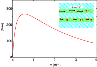
Figure 4: The effective electric field in a 2D-channel with liquid as a function of the flow velocity in second 2D-channel for identical liquids in both channels. The temperature $T=300$ K, the ion concentration in liquid $N_{0}=10^{24}$m^-3, the thickness of the channels $d_{c}=10$ nm, the diffusion coefficients of ions $D=10^{-9}$m²/s and the dielectric constant of the liquid $\varepsilon_{c}=80$. The dielectric constant of the dielectric in the gap between channel $\varepsilon=10$ and the separation between the channels $d=175$ Å.

For comparison with [2D-electron]–[2D-electron] and [2D-electron]–[2D-liquid] configurations, for the [2D-liquid]–[2D-liquid] configuration the effective electric field is many orders of magnitude larger, and depends nonlinerly on the liquid flow velocity $v$.

III van der Waals frictional drag in a 2D- system induced by liquid flow in a semi-infinite chamber

Let us consider a 2D-electron system, isolated from a semi-infinite liquid flow by a dielectric layer with the thickness $d$. For the 2D- electron system the reflection amplitude is determined by Eqs. (2) - (4). To find the reflection amplitude for interface between the dielectric and the liquid we will assume that the liquid fills half-space $z\geq 0$, and that the half-space with $z<0$ is filled by a dielectric with the dielectric constant $\varepsilon$. Let us study the reflection of an electromagnetic wave from the surface of the liquid in the nonretarded limit, which formally corresponds to the limit $c\rightarrow\infty$. In the region $z<0$ the potential can be written in the form

$$\varphi_{q}=(e^{-qz}-Re^{qz})e^{i\mathbf{q\cdot x}-i\omega t},$$ (10)

where $q$ is the magnitude of the component of the wave vector parallel to surface. We will assume that the liquid consists of ions of two types $a$ and $b$. The equation of continuity for the ions

$$-i\omega n_{i}+\mathbf{\nabla}\cdot\mathbf{J}_{i}=0,$$ (11)

where $i=a,b$, $n_{i}=N_{i}-N_{0}$, where $N_{i}$ and $N_{0}$ are the concentration of ions in the presence and absence of the electric field, respectively. To linear order in the electric field

$$\mathbf{J}_{i}=-N_{0}\mu_{i}Q_{i}\mathbf{\nabla}\varphi-D_{i}\mathbf{\nabla}n_{i},$$ (12)

where $D_{i}$ is the diffusion coefficient, $\mu_{i}$ is the mobility and $Q_{i}$ is the charge for ions of type $i$. The diffusion coefficient and the mobility are related with each other by the Einstein relation: $D_{i}=k_{B}T\mu_{i}$. We consider the case when the different ion mobilities differ considerably. In this case, in the calculation of dielectric response it is possible to disregard the diffusion of the less mobile ions. Omitting the index $i$ for the more mobile ions, after substitution of (12) in (11) we obtain

$$i\omega n+D\nabla^{2}\left(n+\frac{N_{0}Q}{k_{B}T}\varphi\right)=0.$$ (13)

This equation must be supplemented with Poisson’s equation

$$\nabla^{2}\varphi=-\frac{4\pi Qn}{\varepsilon_{0}},$$ (14)

where $\varepsilon_{0}$ is the dielectric permeability of the liquid. The general solution of equations (13) and (14) can be written in the form

$$\varphi=(C_{1}e^{-\lambda z}+C_{2}e^{-qz})e^{i\mathbf{q\cdot x}},$$ (15)

where $\lambda=\sqrt{q^{2}+q_{D}^{2}-i\omega/D}$ and $q_{D}=\sqrt{4\pi N_{0}Q^{2}/\varepsilon_{0}k_{B}T}$. At the interface ($z=0$) the electric potential and the normal component of the electric displacement field must be continuous, and the normal component of the flow density must vanish. From these boundary conditions we obtain

$$C_{1}+C_{2}=1-R,$$ (16)

$$-\varepsilon_{0}(\gamma C_{1}+qC_{2})+\varepsilon q(1+R)=0,$$ (17)

$$i\omega\gamma C_{1}+Dq_{D}^{2}qC_{2}=0.$$ (18)

From (16)-(18) we get

$$R=\frac{\epsilon-1}{\epsilon+1},$$ (19)

where

$$\epsilon=\frac{\varepsilon_{0}\lambda(Dq_{D}^{2}-i\omega)}{\varepsilon(Dq_{D}^{2}q-i\omega\lambda)}.$$ (20)

For $v\ll v_{F}$ the frictional drag force acting on the electrons in the 2D- system, due to the interaction with the ions in the liquid, increases linearly with the fluid velocity $v$. In particular, for $N_{0}=10^{24}$m^-3, $T=273$ K, $\varepsilon_{0}=80$, $D=10^{-9}$m²/s, for a high electron density ($n_{s}=10^{19}$m^-2) in the 2D- electron system, $E=1.4\cdot 10^{-6}v$ V/m. This effective electric field is three orders of magnitude larger than obtained for two 2D- electron systems with high electron concentration, and of the same order of magnitude as friction between two 2D- electron systems with low electron concentration.

Fig. 5 shows the dependence of the effective electric field in the 2D- channel on the velocity of the liquid flow in the semi-infinite chamber, for identical liquid in the channel and in the chamber. We have used the same parameters as above for the liquid, with the separation between the channel and chamber $d=1$nm. The effective electric field in the channel initially increases with the flow velocity, reaches a maximum, and then decreases, in agreement with the model calculation in Das . The position of the maximum decreases when the density of ions decreases. The frictional drag force induced by the liquid flow in the narrow channel is 9 orders of magnitude larger than the frictional drag force induced in a 2D-electron system.

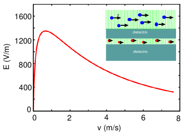
Figure 5: The effective electric field in a 2D-channel with liquid induced by liquid flow in a semi-infinite chamber as a function of the flow velocity for identical liquids in the channel and in the chamber. The temperature $T=300$ K, the ion concentration in liquid $N_{0}=10^{24}$m^-3, the thickness of the channel $d_{c}=10$ nm, the diffusion coefficients of ions $D=10^{-9}$m²/s and the dielectric constant of the liquid $\varepsilon_{0}=80$. The dielectric constant of the dielectric in the gap between channel $\varepsilon=10$ and the separation between the channel and semi-infinite chamber $d=1$ nm.

IV van der Waals frictional drag in a 2D- system induced by liquid flow in an infinite chamber

As a limiting case of the situation considered above, let us consider a 2D-system immersed in a flowing liquid in an infinite chamber. We assume that the liquid flows along the $x$-axis, and that the plane of 2D-system coincides with the $xy$- plane. According to the fluctuation-dissipation theorem, for an infinite medium the correlation function for the Fourier components of the longitudinal current density is determined by RMP07

$$<j_{k}^{f}j_{k}^{f*}>_{\omega}=\frac{\hbar}{(2\pi)^{2}}[n(\omega)+1/2]\omega^{2}\mathrm{Im}\varepsilon(\omega,k),$$ (21)

where $\mathbf{k}=(\mathbf{q},k_{z})$ is the wave vector. The longitudinal current density is connected with the charge density $\rho_{k}=kj_{k}/\omega$ via the continuity equation, from which one obtain

$$<\rho_{k}^{f}\rho_{k}^{f*}>_{\omega}=\frac{\hbar}{(2\pi)^{2}}[n(\omega)+1/2]k^{2}\mathrm{Im}\varepsilon(\omega,k).$$ (22)

Poisson’s equation for the electric potential gives

$$\varphi_{k}^{f}=\frac{4\pi\rho_{k}}{k^{2}\varepsilon(\omega,k)}.$$ (23)

In the $xy$-plane the q - component of the electric potential is determined by

$$\varphi^{f}(\omega,q,0)=\int\frac{dk_{z}e^{ik_{z}0^{+}}}{2\pi}\varphi_{k}^{f}.$$ (24)

From (22) and (23) we get

$$<\varphi^{f}(\omega,q,0)\varphi^{*f}(\omega,q,0)>=4\hbar(n(\omega)+1/2)\mathrm{Im}\Sigma(\omega,q,0),$$ (25)

where

$$\Sigma(\omega,q,0)=-\int_{-\infty}^{\infty}\frac{dk_{z}}{2\pi}\frac{1}{k^{2}\varepsilon_{0}\varepsilon(\omega,k)}.$$ (26)

Taking into account that $E_{q}=iq\varphi_{q}$ we get $<E^{f}_{q}E^{*f}_{q}>_{\omega}=q^{2}<\varphi^{f}_{q}\varphi^{*f}_{q}>_{\omega}$. From the diffusion and Poisson’s equations we get

$$\frac{i\omega}{D}\rho_{k}=k^{2}\left(\rho_{k}+\frac{N_{0}Q^{2}}{k_{B}T}\varphi_{k}\right),$$ (27)

$$\varepsilon_{0}k^{2}\varphi_{k}=4\pi\rho_{k}+4\pi\rho_{k}^{f}.$$ (28)

From (27) and (28) we get the dielectric function of the Debye plasma

$$\varepsilon(\omega,k)=1+\frac{q_{D}^{2}}{k^{2}-i\omega/D}.$$ (29)

Substituting (29) in (26) gives

$$\Sigma(\omega,q)=-\frac{1}{\varepsilon_{0}(q_{D}^{2}-i\omega/D)}\left[-\frac{i\omega/D}{2q}+\frac{q_{D}^{2}}{2\gamma}\right].$$ (30)

According to the fluctuation-dissipation theorem, the average value of the correlation function for the Fourier components of the fluctuating surface charge density in the 2D-system is determined by RMP07

$$<\tau_{q}^{f}\tau_{q}^{f*}>_{\omega}=\frac{\hbar q^{2}}{\pi\omega}(n(\omega)+1/2)\mathrm{Re}\sigma(\omega,q).$$ (31)

If the 2D- system is surrounded by liquid flow the electric field created by the fluctuations of the charge density in the fluid will induce surface charge density fluctuations in the 2D- system. The spectral correlation functions (27) and (31) are determined in the rest reference frame of the liquid, and of the 2D-system, respectively. In order to find the connection between the electric fields in different reference frames we use the Galileo transformation which leads to the Doppler frequency shift of the electrical field in the different reference frames. The electric field in the plane of the 2D- system, due to the fluctuations of the charge density in the liquid, will take the form

$$E(\mathbf{x},t)=e^{-i(\omega+q_{x}V)t+i\mathbf{q\cdot x}}E_{q}^{I},$$ (32)

where $E_{q}^{I}$ is the sum of the electric fields created by the fluctuations of the charge density in the fluid and the induced charge density in the 2D- system:

$$E_{q}^{I}=E_{q}^{f}+4\pi iq\Sigma(\omega,q)\tau^{I}_{q}(\omega^{+}),$$ (33)

where $\omega^{+}=\omega+q_{x}V$ and $\tau^{I}_{q}$ is the surface induced charge density. According to Ohm’s law

$$j_{q}^{I}=\sigma_{q}^{+}E_{q}^{I}=\sigma_{q}^{+}(E_{q}^{f}+4\pi iq\Sigma(\omega,q)\tau^{I}_{q}(\omega^{+})),$$ (34)

where $\sigma_{q}^{+}=\sigma(\omega^{+},q)$ is the longitudinal conductivity for the 2D-system. The continuity equation for the surface charge density gives $j_{q}^{ind}=\omega^{+}\tau^{ind}_{q}/q$ and from (34) we get

$$\tau_{q}^{I}=\frac{q}{\omega^{+}}\frac{\sigma_{q}^{+}E_{q}^{f}}{1-4\pi iq^{2}\sigma_{q}^{+}/\omega^{+}\Sigma(\omega,q)}$$ (35)

and

$$E^{I}_{q}=\frac{E_{q}^{f}}{1-4\pi iq^{2}\sigma_{q}^{+}/\omega^{+}\Sigma(\omega,q)}.$$ (36)

In order to find the electric field created by the charge density fluctuations in the 2D- system it is necessary to solve Poisson’s equation in the rest reference frame of the liquid. In this reference frame the charge density takes the form

$$\tau(\mathbf{x},t)=e^{-i(\omega-q_{x}V)t+i\mathbf{q\cdot x}}\tau_{q}^{II}.$$ (37)

Note that the charge density is composed from the fluctuating $\tau^{f}$ and induced $\tau^{ind}$ charge density: $\tau_{q}^{II}=\tau_{q}^{f}+\tau_{q}^{ind}$. In the presence of the liquid flow the electric field in the plane of the 2D- system, due to the fluctuating surface charge density, is determined by

$$E_{q}^{II}=4\pi iq\Sigma(\omega^{-},q)(\tau_{q}^{ind}+\tau_{q}^{f}),$$ (38)

where $\omega^{-}=\omega-q_{x}V$. From Ohm’s law we get the following expression for the induced charge density

$$\tau_{q}^{ind}=\frac{4\pi iq^{2}\sigma(\omega,q)\Sigma(\omega^{-},q)}{\omega}\frac{\tau^{f}}{1-4\pi iq^{2}\sigma_{q}\Sigma(\omega^{-},q)/\omega}.$$ (39)

Substituting (39) in (38) we get

$$E_{q}^{II}=\frac{4\pi iq\Sigma(\omega^{-},q)\tau^{f}}{1-4\pi iq^{2}\sigma_{q}\Sigma(\omega^{-},q)/\omega}$$ (40)

and

$$\tau_{q}^{II}=\frac{\tau^{f}}{1-4\pi iq^{2}\sigma_{q}\Sigma(\omega^{-},q)/\omega}.$$ (41)

The friction force per unit area of the 2D-system is given by

$$\sigma_{\|}=\int^{\infty}_{-\infty}d\omega\int\frac{d^{2}\mathbf{q}}{(2\pi)^{2}}\frac{q_{x}}{q}<E_{q}\tau_{q}^{*}>_{\omega},$$ (42)

where $E_{q}=E_{q}^{I}+E_{q}^{II}$ and $\tau=\tau^{I}+\tau^{II}$. Substituting (35), (36) and (40), (41) in (42) we get

$$\sigma_{\|}=\frac{2\hbar}{\pi^{2}}\int_{-\infty}^{\infty}dq_{y}\int_{0}^{\infty}dq_{x}q_{x}q^{2}\Big{\{}\int_{0}^{\infty}d\omega[n(\omega)-n(\omega+q_{x}v)]$$

$$\times\left(\frac{\mathrm{Re}\sigma(\omega+q_{x}v)\mathrm{Im}\Sigma(\omega,q)}{(\omega+q_{x}v)\mid 1-4\pi iq^{2}\sigma(\omega+q_{x}v)\Sigma(\omega,q)/(\omega+q_{x}v)\mid^{2}}+\left(\omega+q_{x}v\leftrightarrow\omega\right)\right)$$

$$-\int_{0}^{q_{x}v}d\omega[n(\omega)+1/2]\Big{(}\frac{\mathrm{Re}\sigma(\omega-q_{x}v)\mathrm{Im}\Sigma(\omega,q)}{(\omega-q_{x}v)\mid 1-4\pi iq^{2}\sigma(\omega-q_{x}v)\Sigma(\omega,q)/(\omega-q_{x}v)\mid^{2}}$$

$$+(\omega-q_{x}v\leftrightarrow\omega)\Big{)}\Big{\}},$$ (43)

where ($\omega\pm q_{x}v\leftrightarrow\omega$) denote the terms which are obtained from the preceding terms by permutations of the arguments $\omega\pm q_{x}v$ and $\omega$. With the same parameters as used above for the liquid, and for the high density 2D-electron system, we get $E=8.1\cdot 10^{-6}v$ V/m. For a 1D-electron system we obtained a formula which is similar to Eq. (43). Fig. 6 shows the result of the calculations of the effective electric field for a 1D-electron system with the electron density per unit length $n_{l}=3\times 10^{9}$m^-1, the temperature $T=300$ K, and with the same parameters for the liquid as used above.

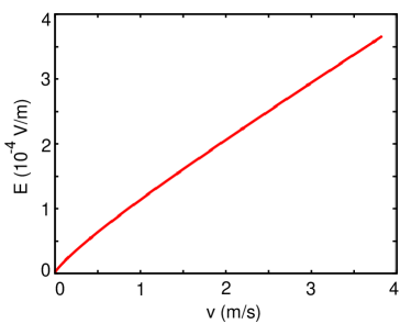
Figure 6: The effective electric field in a 1D-electron system induced by liquid flow in a infinite chamber, as a function of the flow velocity. For the same parameters for the liquid as in Fig. 5. The electron concentration per unit length in 1D-system $n_{l}=3\cdot 10^{9}$m^-1 and the electron relaxation time $\tau=4\cdot 10^{-14}$s

For the 1D-electron system we obtained a slight deviation from the linear dependence of the frictional drag on the liquid flow velocity. The frictional drag for the 1D-electron system is one order of magnitude larger than for the 2D-electron system.

Fig. 7 shows the dependence of the effective electric field in the liquid in the 2D-channel on the liquid flow velocity in the infinite chamber, assuming identical liquid in the channel and in the chamber. Qualitatively, we obtained the same results for a 1D-channel.

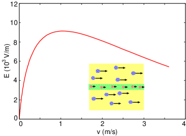
Figure 7: The same as Fig. 5 but for infinite chamber.

V Discussion and conclusion

For a channel with open ends the frictional drag force will induce a drift motion of the ions in the liquid with the velocity $v_{d}=D_{c}QE/k_{B}T$. The positive and negative ions will drift in the same direction. If ions have different mobility then the drifting ions will lead to an electric current whose direction will be determined by the current created by the ions with the largest mobility. For a channel with closed ends the frictional drag force will lead to a change in ion concentration along the channel. In the case of ions with the different mobilities, the friction force will be different for the ions with the opposite charges. As a result the ions of opposite charges will be characterized by different distribution functions which, as for electronic systems, will result in an electric field, and an induced voltage which can be measured. Let us write the friction force acting on the ions of different type in the form: $F_{a}=QE_{a}$ and $F_{b}=QE_{b}$. From the condition that, in the static case, the flux density in the channel must vanish, we get

$$n_{a}=-\frac{Q}{k_{B}T}\left(\varphi-E_{a}x\right),$$ (44)

$$n_{b}=\frac{Q}{k_{B}T}\left(\varphi+E_{a}x\right).$$ (45)

These equation must be supplemented with Poisson’s equation

$$\frac{d^{2}\varphi}{d^{2}x}=-\frac{4\pi Q}{\varepsilon_{c}}(n_{a}-n_{b}).$$ (46)

Substituting (44)-(45) in (46) we get

$$\frac{d^{2}\varphi}{d^{2}x}=q_{D}^{2}\left(2\varphi-\Delta Ex\right),$$ (47)

where $\Delta E=E_{a}-E_{b}$. The solution of (47) with boundary condition

$$\frac{d\varphi}{dx}\Big{|}_{x=\pm L/2}=0,$$ (48)

where $L$ is the channel length, has the form

$$\varphi(x)=\frac{\Delta E}{2}\left(x-\frac{1}{\sqrt{2}q_{D}}\frac{\sinh{\sqrt{2}q_{D}x}}{\cosh\sqrt{2}q_{D}L/2}\right).$$ (49)

The voltage between the ends of the channel is determined by

$$U=\varphi(L/2)-\varphi(-L/2)=\Delta E\left(\frac{L}{2}-\frac{1}{\sqrt{2}q_{D}}\tanh{\sqrt{2}q_{D}L/2}\right).$$ (50)

For $q_{D}L\gg 1$ the voltage, which appears as a result of the frictional drag, will be approximately equal to $U\approx\Delta{E}L/2$. Furthermore, the frictional drag will induce a pressure difference $\Delta p=nLeE$. For example, if $N_{0}=10^{24}$m^-3, $L=100\mu$m and $E=1000$V/m we get pressure difference $\Delta p=10^{4}$ Pa, which should be easy to measure. Assume now that one type of ions are fixed (adsorbed) on the walls of the channel and an equal number of mobile ions of opposite sign are distributed in the liquid phase. In this case the motion of the polar liquid in the adjacent region will lead to frictional drag force acting on the mobile ions in the channel. For a channel with the closed ends this frictional drag will induce a voltage, which can be measured.

In this paper we have shown that the van der Waals frictional drag force, induced in low-dimensional system by liquid flow, can be several orders of magnitude larger than the friction induced by an electron current. For narrow 2D-and 1D-channels with liquid the frictional drag force is several orders of magnitude larger than for 2D-and 1D-electron systems. In the contrast to electron systems, the frictional drag force for a narrow channel with liquid depends nonlinearly on the flow velocity. These results contradict to the calculations in Ref. Kumar2 , where it was assumed that the observed nonlinear dependence of a voltage on the liquid flow velocity was connected with the frictional drag acting on the electrons in the nanotubes. However, according to our calculations, the mobile ions in the channels of porous medium experience considerably greater frictional drag force due to van der Waals friction, than on the electrons in low-dimensional electronic structures. Thus, the liquid flow induced voltage observed in Kumar2 is more likely connected with the frictional drag experienced by mobile ions in an electrolyte in the channels between nanotubes, rather than the electrons in the nanotubes. These results should have a broad application for studying of the van der Waals friction and in the design of nanosensors. Such detectors would be of great interest in micromechanical and biological applications Schasfoort ; Munro , where local dynamical effects are intensively studied.

Acknowledgment

A.I.V acknowledges financial support from the Russian Foundation for Basic Research (Grant N 08-02-00141-a) and DFG.

References

- (1) K. Joulain, J. P. Mulet, F. Marquier, R. Carminati, and J. J. Greffet, Surf. Sci. Rep. , 57, 59 (2005)
- (2) A. I. Volokitin and B. N. J. Persson, Rev. Mod. Phys. 79 (3) (2007)
- (3) B. C. Stipe, H. J. Mamin, T. D. Stowe, T. W. Kenny, and D. Rugar, Phys. Rev. Lett. 87, 096801 (2001).
- (4) S. Kuehn, R. F. Loring, and J.A. Marohn, Phys. Rev. Lett. 96, 156103 (2006).
- (5) A. I. Volokitin and B. N. J. Persson, Phys. Rev. Lett. 94, 086104 (2005).
- (6) A. I. Volokitin, B. N. J. Persson, and H. Ueba, Phys. Rev. B 73, 165423 (2006).
- (7) M. B. Pogrebinskii, Fiz.Tekh.Poluprov. 11, 637 (1977) [Sov.Phys. Semicond. 11, 372 (1977)].
- (8) P. J. Price, Physica B+C 117, 750 (1983).
- (9) T. J. Gramila, J. P. Eisenstein, A. H. MacDonald, L.N. Pfeiffer, and K. W. West, Phys. Rev. Lett. 66, 1216 (1991).
- (10) U. Sivan, P. M. Solomon, and H. Shtrikman, Phys. Rev. Lett. 68, 1196 (1992).
- (11) M. C. Bønsager, K. Flensberg, Ben Yu-Kuang. Hu, and A. H. Macdonald, Phys.Rev. B 57, 7085 (1998).
- (12) S. Ghosh, A. K. Sood, and N. Kumar, Science 299, 1042 (2003).
- (13) S. Ghosh, A. K. Sood, S. Ramaswamy, and N. Kumar, Phys.Rev. B 70, 205423 (2004).
- (14) A. E. Cohen, Science, 300, 1235 (2003).
- (15) S. Ghosh, A. K. Sood, and N. Kumar, Science 300, 1235 (2003).
- (16) P. Král and M. Shapiro, Phys. Rev. Lett. 86, 131 (2001).
- (17) M. Das, S. Ramaswamy, A. K. Sood, and G. Ananthakrishna, Phys. Rev. E 73, 061409(2006).
- (18) B. N. J. Persson, U. Tartaglino, E. Tosatti, and H. Ueba, Phys.Rev. B 69, 235410 (2004).
- (19) A. I. Volokitin and B. N. J. Persson, Phys. Rev. B 77, 033413 (2008)
- (20) A. I. Volokitin and B. N. J. Persson, J.Phys.: Condens. Matter 11, 345 (1999);Phys.Low-Dim.Struct.7/8,17 (1998)
- (21) A. I. Volokitin and B. N. J. Persson, J.Phys.: Condens. Matter 13, 859 (2001)
- (22) N. D. Mermin, Phys. Rev. B 1, 2362 (1970)
- (23) F. Stern, Phys. Rev. Lett. 18, 546 (1967)
- (24) R. B. M. Schasfoort, S. Schlautmann, J. Hendrikse, and A. van der Berg, Science 286, 942 (1999).
- (25) N. J. Munro, K. Snow, J. A. Kant, and J. P. Landers, Clin. Chem. 45, 1906 (1999).