Quantum Back Reaction to asymptotically AdS Black Holes

Abstract

We analyze the effects of the back reaction due to a conformal field theory (CFT) on a black hole spacetime with negative cosmological constant. We study the geometry numerically obtained by taking into account the energy momentum tensor of CFT approximated by a radiation fluid. We find a sequence of configurations without a horizon in thermal equilibrium (CFT stars), followed by a sequence of configurations with a horizon. We discuss the thermodynamic properties of the system and how back reaction effects alter the space-time structure. We also provide an interpretation of the above sequence of solutions in terms of the AdS/CFT correspondence. The dual five-dimensional description is given by the Karch-Randall model, in which a sequence of five-dimensional floating black holes followed by a sequence of brane localized black holes correspond to the above solutions.

I Brane world black holes and the AdS/CFT correspondence

The AdS/CFT conjecture relates the gravitational dynamics of a $(d+1)$-dimensional AdS spacetime to a $d$-dimensional conformal field theory (CFT), and it was initially formulated as a correspondence between type IIB supergravity on $\mbox{AdS}_{5}\times\mbox{S}^{5}$ and ${\cal N}=4$ $U(N)$ super Yang-Mills (SYM) theory, with coupling $\hat{g}$ and ’t Hooft parameter $\lambda=\hat{g}^{2}N$, related to the supergravity parameters by

$$\ell=\lambda^{1/4}\ell_{s}~{},~{}~{}~{}~{}{\ell^{3}\over G_{5}}={N^{2}\over\pi}~{}.$$ (1)

In the above formulas $\ell_{s}$ is the string length, $\ell$ and $G_{5}$ are the five-dimensional AdS curvature length and Newton constant, respectively Mal ; Wit ; Gub . The correspondence relates the supergravity partition function in AdS₅ to the generating functional $W_{CFT}$ of connected Green’s functions for the CFT on the boundary, and it has a very interesting connection with the Randall-Sundrum (RS) model RS .

The RS model consists of two copies of a part of AdS₅-like spacetime. The boundaries of the copies are glued with a positive tension brane. The model is described by the following action:

$$S_{RS}=S_{EH}+S_{\text{brane}}+S_{M}~{},$$ (2)

where $S_{EH}$ is the five-dimensional Einstein-Hilbert action, $S_{\text{brane}}$ represents the action of the brane with tension $\sigma=3/4\pi G_{5}\ell$, and $S_{M}$ describes matter confined on the brane. On the four-dimensional brane, asymptotically flat spacetime is realized by tuning the brane tension relative to the negative bulk cosmological constant. The Standard Model is localized on the brane, and the observed four-dimensional nature of gravity arises owing to the presence of a localized graviton zero mode GT .

References Gubser2 ; Hawking provided an interpretation of the RS model in terms of the AdS/CFT correspondence. The correspondence implies

$$S_{\text{RS}}=-{\ell\over 16\pi G_{5}}\int d^{4}x\sqrt{g}R+2W_{CFT}+S_{M}~{},$$ (3)

indicating that the classical gravity in the RS model is dual to four-dimensional gravity coupled to a cutoff CFT. From the above action, the effective four-dimensional Newton constant is read as

$$G_{4}={G_{5}\over\ell}.$$ (4)

In the linearized, weak gravity regime various results clearly support this conjecture Hawking ; Duff ; TanakaFRWGW ; PujolasDW . On the other hand, although some evidence for the conjecture exists (e.g. tanaka ), things become more complicated when trying to extend the correspondence to the non-linear regime in general Shiromizu ; GarrigaSasaki , and to black holes in particular. In this paper we will be concerned with the latter case.

Let us summarize the present understanding of black hole solutions in the RS model. In this model no large, stable, static black hole solution localized on the brane has so far been found, whereas small localized solutions have been constructed numerically Kudo1 for black holes with size smaller than the curvature scale $\ell$ .

This situation can be interpreted in the light of the AdS/CFT correspondence, and in Refs. emparan ; tanaka it has been conjectured that large stable black holes localized on the brane do not exist in the RS model. The intuitive picture is as follows. Consider a four-dimensional black hole with CFT. This black hole will evaporate into CFT modes. If the correspondence is valid also in this situation, this evaporation process must be equivalent to a classical five-dimensional dynamical phenomena. This may imply that there is no stationary black hole solution in the five-dimensional RS model, and that the five-dimensional black hole “evaporates” by a classical process. Note that existence of the numerical solutions of Ref. Kudo1 , describing small black holes, is not in contradiction with the above statement since the correspondence is not expected to hold below the cutoff length scale of the CFT, which is of order of the AdS curvature scale $\ell$.

Black holes floating in the bulk are also expected to exist tanaka , although no solution of this sort has been found. Such floating black holes also cannot be large for the following reason. In the RS model, the gravitational force between the brane and a particle in the bulk is repulsive. Writing the metric in Poincaré coordinates,

$$ds^{2}=dy^{2}+e^{-2y/\ell}\left(-d\bar{t}^{2}+d{\bf\bar{x}}^{2}\right)~{},$$ (5)

one can see that the acceleration of a particle is $a=-\partial_{y}\log\sqrt{-g_{\bar{t}\bar{t}}}=1/\ell$ and independent of $y$. The only force that compensates such repulsive force is the self-gravity of the mirror image of the particle on the other side of the brane. From the above observation, we expect that, as $\ell$ decreases, the equilibrium position of the floating black hole should move towards the brane. However, the attractive force between the black holes is at most of $O(1/r_{\rm h})$, with $r_{\rm h}$ being the horizon size. If $r_{\rm h}\gg\ell$, such attractive force will not be sufficient to cancel the repulsive force from the brane. Thus, large black holes will necessarily touch the brane.

Although the difficulty in constructing large localized (or floating) black hole solutions in the RS model synchronizes with the prediction from the AdS/CFT correspondence, it is also true that larger black holes become more difficult to construct simply for a technical reason because two different scales, the bulk curvature scale $\ell$ and the black hole size, should be resolved simultaneously. Therefore it is difficult to prove the absence of solutions numerically. Then, one of the authors proposed to study black holes in Karch-Randall (KR) model KR , in which the brane tension is chosen to be less than the fine-tuned value of the RS model tanaka2 . Unperturbed background bulk geometry is AdS, which is conveniently described by

$$ds^{2}=dy^{2}+\ell^{2}\cosh^{2}\left(y/\ell\right)ds^{2}_{AdS_{4}}~{},$$ (6)

where $ds^{2}_{AdS_{4}}$ is the line element of four-dimensional AdS spacetime with unit curvature:

$$ds^{2}_{AdS_{4}}=-\left(1+{\bar{r}^{2}}\right)d\bar{t}^{2}+\left(1+{\bar{r}^{2}}\right)^{-1}d\bar{r}^{2}+\bar{r}^{2}d\Omega_{2}^{2}.$$ (7)

Contrary to the Poincare chart convenient for RS model, in this chart the warp factor is not monotonic but has a minimum at $y=0$. The position of the brane is specified by $y=y_{b}$, and $y_{b}$ is determined by the condition

$$\sigma=-{3\over 4\pi G_{5}\ell}\tanh\left(y_{b}/\ell\right)~{}.$$ (8)

The RS limit is obtained by letting $y_{b}\rightarrow-\infty$.

Let us consider a small black hole floating in the bulk of the KR model. Following the same analogy as before, we can look at the acceleration of a small mass particle. In this case a particle feels a potential

$$U_{\text{eff}}=\log\left(\cosh{y\over\ell}\right)+U_{\text{sg}}~{},$$ (9)

where $U_{\text{sg}}$ is the self-gravitational part caused by its own mirror image on the other side of the brane. The profile of $U_{\text{eff}}$ is illustrated in Fig. 1 and suggests that there will be two small black hole solutions: an unstable one close to the UV brane, and a stable one near $y=0$, far from the UV brane. In the RS limit $\delta\sigma\rightarrow 0$, the latter is infinitely far from the brane and hence it does not exist. It is natural to imagine that the stable floating black holes also touch the brane when the size becomes big enough.

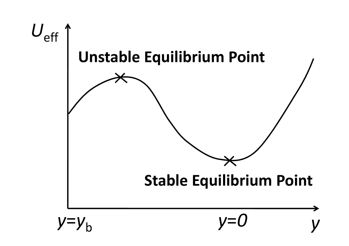
Figure 1: Effective potential in the KR model.

According to the AdS/CFT correspondence, we may expect that a five-dimensional black hole in the KR model will be dual to some object in the four-dimensional gravity coupled to CFT with negative cosmological constant tanaka2 . Naive expectation is that a brane-localized black hole and a floating black hole in the KR model are, respectively, dual to a four-dimensional black hole with back reaction of CFT halo and a star composed of CFT, which we refer to in this paper as a quantum black hole and a CFT star. If this duality is really the case, we can examine black holes in the KR model by analyzing the four-dimensional system.

On the four-dimensional brane in the KR model, asymptotically AdS spacetime is realized. Under the restriction to static and spherically symmetric configurations, the four-dimensional metric is in general written as

$$ds^{2}=-\alpha(r)^{2}dt^{2}+V(r)^{-1}dr^{2}+r^{2}d\Omega_{2}^{2}~{}.$$ (10)

As we consider an equilibrium configuration with a black object in the bulk, the corresponding CFT is also expected to be in thermal equilibrium at a finite temperature. The local temperature of CFT in equilibrium red-shifts as

$$T_{\rm local}(r)=T/\alpha(r),$$ (11)

where the global temperature of the system $T$ is defined with respect to the time-like Killing vector $\partial/\partial t$.

Let us consider a quantum black hole in the above thermal AdS spacetime. For black hole configurations in equilibrium the appropriate vacuum state will be the Hartle-Hawking state. In the asymptotically flat case, back reaction due to CFT is too strong to keep the asymptotic structure of the spacetime unchanged (the total mass diverges). In the asymptotically AdS case, a non-zero cosmological constant changes the situation dramatically. Since the lapse function in AdS behaves as $\alpha\sim r/L$ for large circumferential radius $r$, where $L$ is the four-dimensional AdS curvature scale, the temperature and hence the energy density of thermal CFT decrease rapidly for $r\gg L$. This reduces the effects of the back reaction. If the black hole size is large, the energy density due to CFT will stay negligibly small at any radius. Whilst, if the size of the black hole is small, the back reaction becomes important and a static black hole solution becomes non-trivial. Roughly speaking, such a small black hole will be unstable against the CFT back reaction and will ‘evaporate’ into a CFT star of the same mass.

The sequence of the CFT stars can be tagged by the central density, and the end-point of the sequence corresponds to a star with singular central density and the lapse vanishing at the center. Thus, this sequence of the CFT stars will naturally flow into the sequence of quantum black holes, whose starting-point corresponds to a small black hole in the limit of zero horizon radius.

We can interpret the sequence of four-dimensional quantum black holes and CFT stars from a five-dimensional view point as follows. At the transition point of the sequence, the lapse vanishes at the center of the system. This four-dimensional configuration corresponds to a five-dimensional black hole floating in the bulk and just touching the brane, since the lapse vanishes at the touching point for this five-dimensional configuration too. In this way, we may speculate that the sequence of floating black holes corresponds to the sequence of CFT stars, while the sequence of brane-localized black holes corresponds to the sequence of quantum black holes.

In this paper, we will present our investigation concerning the four-dimensional asymptotically AdS quantum black holes and CFT stars with the aim of clarifying the phase diagram structure of black objects in the KR model. We will give quantitative estimates of the characteristic quantities of the model by explicitly constructing equilibrium configurations in the dual picture described by four-dimensional gravity with CFT correction. In Sec. II, we will show that the effects of CFT can be properly approximated by a radiation fluid. We analyze properties of CFT in Schwartzschild AdS spacetime and give the conditions for the radiation fluid approximation to CFT to be applicable. We will show that those four-dimensional objects in equilibrium state can be well approximated by this approximation, as long as we restrict our interest to the range of parameters where the correspondence is expected to be valid. In Sec. III, we will illustrate our method to construct equilibrium configurations of four-dimensional self-gravitating CFT and study its basic properties that can be derived analytically. The full numerical analysis will be given in Sec. IV. Based on the above results, we will finally discuss the implications for the KR model via the AdS/CFT correspondence in Sec. V and summarize the paper in Sec. VI.

For notation convenience, we set $G_{4}$ to unity from Sec. II to Sec. IV.

II CFT Energy-Momentum Tensor and Radiation fluid approximation

In order to study the effects of the back reaction, explicit knowledge of the quantum energy-momentum tensor of the CFT in the Hartle-Hawking vacuum state is necessary. The computation is, however, technically very complicated and, apart from Ref. flachitanaka where the vacuum polarization has been obtained for a conformal scalar field, we are not aware of other relevant results for Schwarzschild AdS black holes in the literature. Even had we obtained the exact expression for the energy-momentum tensor, additional problems would arise in solving the Einstein equations self-consistently. The energy momentum tensor of CFT effectively contains higher derivatives of the metric functions, and those terms will introduce spurious solutions and make the choice of boundary conditions quite non-trivial. For this reason, as a first step, it seems natural to look for a simplified scheme to take into account the quantum back reaction approximately. In this paper we propose to use the radiation fluid approximation, which makes it easy to study back reaction effects of CFT on the spacetime structure. In this section we evaluate the CFT energy-momentum tensor using Page’s approximation page on the Schwarzschild AdS black hole background gregory , and compare the results with those obtained by the radiation fluid approximation.

Before introducing Page’s approximation, it is instructive to discuss the relevant length scales. Since the CFT is scale invariant, the only scales that characterize the system are (i) geometrical length scales of the space-time, such as the distance from the BH horizon radius $r-\bar{r}_{\rm h}$ or the curvature scale, and (ii) the scale related to the local temperature of the system $1/T_{\rm local}$. For high enough temperatures, $1/T_{\rm local}$ becomes the only relevant length scale of the system, except for the vicinity of the horizon. In this case, from the symmetry, the energy momentum tensor of CFT should follow a Stephan-Boltzmann law,

$$T^{\mu}{}_{\nu}=\frac{\pi^{2}}{30}g_{\rm eff}T_{\rm local}^{4}(\delta^{\mu}{}_{\nu}-4\delta^{\mu}{}_{0}\delta^{0}{}_{\nu})~{},$$ (12)

where $g_{\rm eff}$ represents the effective number of degrees of freedoms. Expression (12) claims that a thermal CFT can be approximated by a radiation fluid when the red-shifted temperature of the system is high enough.

The procedure is, however, not straightforward, since the radiation fluid approximation breaks down near the horizon, due to the fact that the local temperature $\propto\alpha^{-1}$ diverges there. In order to remove this pathology, we need to consider the quantum contribution to the energy momentum tensor, and will use Page’s approximation for this purpose. We split the genuine energy density into two parts, $\rho=\rho_{\rm r}+\rho_{\rm q}$, where $\rho_{\rm r}$ corresponds to a classical radiation fluid contribution and $\rho_{\rm q}$ to a quantum contribution that is defined by the remainder of this section.

As an example, we consider a conformal scalar field on Schwarzschild AdS background. In this case Page’s approximation is known to be equivalent to the fourth order WKB approximation anderson . In order to take into account all the degrees of freedom of SYM, conformal spinor and vector contributions should be included. However, Page’s approximation produces unphysical divergences on the event horizon for these cases, and to include such contributions rigorously, a more sophisticated numerical method is needed anderson . We do not pursue this rather technically complicated issue here. For a conformal scalar field, the classical part $\rho_{\rm r}$ described by a radiation fluid is given by

$$\rho_{\rm r}={r^{2}\over K\bar{r}_{\rm h}^{4}}(1+3\bar{r}_{\rm h}^{2}/L^{2})^{4}~{},$$ (13)

while the quantum part $\rho_{\rm q}$ is computed by using Page’s approximation as

$$\rho_{\rm q}=-{1\over K}\sum_{i=0}^{9}a_{i}r^{i-6}~{},$$ (14)

with

$$K\equiv 7680\pi^{2}\left(r-\bar{r}_{\rm h}\right)^{2}\left\{1+\left(r^{2}+\bar{r}_{\rm h}r+\bar{r}_{\rm h}^{2}\right)/L^{2}\right\}^{2}~{}.$$

The coefficients $a_{i}$ are polynomials in $\chi\equiv\bar{r}_{\rm h}/L$ of degree smaller than 9:

$$a_{0} =33\bar{r}_{\rm h}^{4}\left(1+\chi^{2}\right)^{4}~{}, a_{1} =-72\bar{r}_{\rm h}^{3}\left(1+\chi^{2}\right)^{3}~{},$$

$$a_{2} =40\bar{r}_{\rm h}^{2}(1+\chi^{2})^{2}~{}, a_{3} =-88\bar{r}_{\rm h}\chi^{2}\left(1+\chi^{2}\right)^{3}~{},$$

$$a_{4} =104\chi^{2}\left(1+\chi^{2}\right)^{2}~{}, a_{5} =0~{},$$

$$a_{6} ={104\over L^{2}}\chi^{2}\left(1+\chi^{2}\right)~{}, a_{7} =-{32\over L^{3}}\chi\left(1+\chi^{2}\right)~{},$$

$$a_{8} ={16\over L^{4}}~{}, a_{9} ={32\over L^{5}}\chi\left(1+\chi^{2}\right)~{}.$$

Let us consider the quantum effects in the near horizon region first. We define an inner critical radius $r_{\rm in}$ as the radius at which the equality

$$|\rho_{\rm q}|=c\rho_{\rm r}$$ (15)

is first satisfied, with $c$ being a constant of order $O(1)$. For $r<r_{\rm in}$ the quantum contribution dominates the classical radiation part. The result is not so sensitive to the choice of $c$ as long as it is $O(1)$. Figure 2 illustrates the relation between the horizon radius $\bar{r}_{\rm h}$ and the inner critical radius $r_{\rm in}$: when $\bar{r}_{\rm h}$ is small compared with the four-dimensional curvature scale $L$, $r_{\rm in}/\bar{r}_{\rm h}$ is approximately constant of $O(1)$ (e.g. $r_{\rm in}\sim 3\bar{r}_{\rm h}/2$ for $c=1/2$); when we increase $\bar{r}_{\rm h}$ beyond $L$, $r_{\rm in}/\bar{r}_{\rm h}$ begins to increase and finally solutions of Eq. (15) cease to exist. No inner critical radius can be defined for larger $\bar{r}_{\rm h}$.

Figure 2: Relation between the horizon radius $\bar{r}_{\rm h}$ and critical radius $r_{\rm in}$. We have set $c=1/2$ and $l/L=10^{-8}$.

Having fixed the critical radius as above, we can discuss the strength of the reaction due to the CFT in the region $r<r_{\rm in}$ by comparing the total energy of the CFT within the critical radius $M_{\rm in}$ with the black hole mass $m_{\rm h}$. When the size of the black hole is small, $M_{\rm in}$ is estimated as $M_{\rm in}\sim(\pi^{2}/30)g_{\rm eff}T_{\rm local}^{4}\bar{r}_{\rm h}^{3}\sim\ell^{2}/\bar{r}_{\rm h}$, where we have substituted

$$g_{\rm eff}=\frac{3}{4}\cdot 15N^{2}~{},$$ (16)

which is the value for ${\cal N}=4$ $U(N)$ SYM theory, and used the relation (1). The factor $3/4$ in Eq. (16) is the empirical factor that explains the discrepancy between results for CFTs in strong and weak coupling cases 3/4factor . Hence, we have

$${M_{\rm in}\over m_{\rm h}}\sim\left(\ell\over\bar{r}_{\rm h}\right)^{2}~{}.$$ (17)

It is easy to see that, as long as $\ell/\bar{r}_{\rm h}$ is small, the above ratio is also small, and the contribution to the total mass of CFT living inside the inner critical radius is negligible. The cases with $\ell>\bar{r}_{\rm h}$ are beyond the range of applicability of the AdS/CFT correspondence and are outside the parameter region of our interest. For illustration, Fig. 3 shows the ratio $M_{\rm in}/m_{\rm h}$ with respect to the horizon radius.

Figure 3: Ratio of the total energy of the CFT inside the critical radius and the black hole horizon radius. We set $\ell^{2}/L^{2}=10^{-8}$.

Let us move on to the quantum effect in the asymptotic region next. At a large distance, the classical radiation part of the energy density $\rho_{\rm r}$ behaves as $1/r^{4}$, whilst the quantum part $\rho_{\rm q}$ behaves as $1/r^{3}$, as is seen from Eq. (14). Hence, the quantum part dominates above an outer critical radius, $r_{\rm out}$, which is defined as before by Eq. (15). By comparing Eqs. (13) and (14), we find $r_{\rm out}\sim L\left(L/\bar{r}_{\rm h}\right)^{5}$ for small black holes with $\bar{r}_{\rm h}\ll L$. This quantum part $\rho_{\rm q}$ in the outer region gives a non-negligible contribution for large $r$. In fact, by taking $\rho_{\rm q}$ into account, the mass measured at $r$, $M(r)$, will be modified as follows. Eq. (14) suggests that the leading term of $\rho_{q}$ behaves as $\sim-M(r)\ell^{2}/L^{2}r^{3}$ when we consider the back reaction of the CFT to the background geometry. Then, $M(r)$ will be modified as

$$M(r)\sim\int^{r}r^{\prime\,2}\rho_{\rm q}dr^{\prime}\sim M(r_{\rm out})\times\left(\frac{r}{r_{\rm out}}\right)^{-\ell^{2}/L^{2}},$$ (18)

where $M(r_{\rm out})$ is the mass in the region $r<r_{\rm out}$. Hence, the effect of $\rho_{\rm q}$ significantly alter the total mass $M$ from the value for the bare black hole at a very large distance. The above result can be interpreted as the mass screening effect due to the non-zero graviton mass of $O(\ell/L^{2})$ porrati ; AdSDuff . To avoid ambiguity of $M$ with respect to $r$, strictly speaking, we need to truncate the model at a finite radius well outside the AdS curvature radius but before this screening effect becomes significant. This prescription will be justified later in Sec. V. As long as this truncated model is concerned, we can neglect the quantum part of the energy density $\rho_{\rm q}$ also in the region $r>r_{\rm out}$. Once we neglect the quantum part, this screening effect is also absent. Hence, in the actual computation discussed in the succeeding sections, where we use the radiation fluid approximation, we do not have to care about this truncation.

As the size of a black hole becomes large compared with $L$, the interval between $r_{\rm in}$ and $r_{\rm out}$ shrinks and eventually disappears. Beyond that point, the classical radiation part of the energy density $\rho_{\rm r}$ does not dominate the quantum part for any $r$. Hence, one may think that the approximating the energy momentum tensor by a radiation fluid is not a good approximation at all. However, in this case the temperature is so low that the back reaction to the mass due to CFT is negligibly small, as long as we adopt the above prescription of truncating the model at a finite radius before the screening effect becomes significant. Hence, we conclude that in all cases that we are interested in the radiation fluid approximation is expected to give a good approximation to the energy momentum tensor of CFT except for the vicinity of the event horizon.

III Boundary theory description of floating black holes

III.1 CFT stars

First, we re-examine spherically symmetric, equilibrium configuration of a radiation star in asymptotically AdS spacetime, which was analyzed in Ref. PP . The only difference from the literature is that the effective number of degrees of freedom $g_{\rm eff}$ is set to a large number $(45/4)N^{2}$ in connection to the AdS/CFT correspondence.

To deal with the above problem, it is convenient to write the metric (10) as

$$ds^{2}=-e^{2\psi}Vdt^{2}+V^{-1}dr^{2}+r^{2}(d\theta^{2}+\sin^{2}\theta d\phi^{2})~{},$$ (19)

with

$$V=1+\frac{r^{2}}{L^{2}}-\frac{2m(r)}{r}~{}.$$ (20)

We re-parametrize the time coordinate $t$ so as to satisfy

$$\lim_{r\to\infty}\psi(r)=0~{}.$$ (21)

In these coordinates the total mass of the system is given by

$$M\equiv\lim_{r\to\infty}m(r)~{},$$

Pressure and energy density can be written as

$$\rho=3P_{r}=3P_{\theta}=\frac{\pi^{2}}{30}g_{\rm eff}T_{\rm local}^{4}=\frac{3\pi^{3}\ell^{2}}{8}T^{4}e^{-4\psi}V^{-2}~{}.$$ (22)

The Einstein equations (with $\Lambda=-3/L^{2}$) are

$$\frac{dm}{dr} = 4\pi r^{2}\rho~{},$$ (23)

$$\frac{d\psi}{dr} = \frac{16\pi}{3}rV^{-1}\rho~{},$$ (24)

$$\frac{d\rho}{dr} = -\frac{4\rho(m+4\pi r^{3}\rho/3+r^{3}/L^{2})}{r^{2}+r^{4}/L^{2}-2rm}~{}.$$ (25)

The central density

$$\rho_{c}\equiv\rho(0),$$ (26)

can be used to parametrize the solutions, and the boundary condition for $m(r)$ is specified by

$$m(0) = 0~{}.$$ (27)

Then, integrating Eqs. (23) and (25) from $r=0$ for given curvature scales $\ell$ and $L$, we obtain a one-parameter family of non-singular equilibrium configurations labelled by $\rho_{c}$. From the boundary condition (21) and the relation (22), we obtain the global temperature

$$T=\lim_{r\to\infty}\Big{(}\frac{8}{3\pi^{3}\ell^{2}}\rho V^{2}\Big{)}^{1/4}~{}.$$ (28)

Finally, the solution of Eq. (24) is obtained algebraically from Eq. (22) as

$$\psi(r)=\frac{1}{4}\ln\Big{(}\frac{3\pi^{3}\ell^{2}}{8}T^{4}\rho^{-1}V^{-2}\Big{)},$$ (29)

without solving Eq. (24). Another global quantity of interest is the total entropy of the system, $S(L,\ell,\rho_{c})$. Once the functional dependence of $M$ and $T$ upon $\rho_{c}$ is determined, $S$ can be obtained by integrating the first law of thermodynamics,

$$dS=\frac{dM}{T}$$ (30)

for fixed $\ell$ and $L$, with $S=0$ at $\rho_{c}=0$.

Notice that, writing the equations in terms of the rescaled variables associated with “$~{}\tilde{}~{}$”, defined by

$$r=L\tilde{r}~{},\quad\rho=L^{-2}\tilde{\rho}~{},\quad m=L\tilde{m},$$ (31)

$L$-dependence is eliminated from the Einstein equations and also from the form of the metric function (20). Accordingly, the rescaled thermodynamic quantities defined by

$$M(L,\ell,\rho_{c}) = L\tilde{M}(L^{2}\rho_{c})~{},$$ (32)

$$T(L,\ell,\rho_{c}) = \ell^{-1/2}L^{-1/2}\tilde{T}(L^{2}\rho_{c})~{},$$ (33)

$$S(L,\ell,\rho_{c}) = \ell^{1/2}L^{3/2}\tilde{S}(L^{2}\rho_{c})~{},$$ (34)

absorb the $\ell$-dependence present in Eq. (22), too. Owing to the above scaling relations, we can set $L=\ell=1$ without loss of generality.

Details of the numerics for the CFT star configurations will be reported in the succeeding section along with the black hole ones. Here we wish to close this subsection with some analytic estimates of the thermodynamic quantities of our interest. As discussed in Ref. PP , when the radiation has negligible self-gravity, the metric will be approximated by the pure AdS spacetime. The condition for the self-gravity to be negligible can be stated as

$$m(r)/r\ll 1,$$ (35)

for all $r$. This condition is satisfied when the central density of the radiation is much smaller than that corresponds to the four-dimensional AdS curvature scale, $(\pi^{2}/30)g_{\rm eff}T^{4}\ll L^{-2}$. The temperature corresponding to the critical central density at which the equality $(\pi^{2}/30)g_{\rm eff}T^{4}=L^{-2}$ is satisfied will then be approximately given by

$$T\sim\ell^{-1/2}L^{-1/2}.$$ (36)

Below this temperature, the spacetime is practically AdS, which will work as a box of the volume of $O(L^{3})$ for the radiation. Then, the total energy of the system can be estimated easily as

$$M\sim\ell^{2}L^{3}T^{4}.$$ (37)

Similarly, the total entropy of the system is approximated by

$$S\sim\ell^{2}L^{3}T^{3}.$$ (38)

Substituting $T\sim\ell^{-1/2}L^{-1/2}$, one can estimate the total mass and the total entropy at the critical point where the back reaction to the geometry becomes important as

$$M/L \sim 1~{},$$ (39)

$$\ell^{-1/2}L^{-3/2}S \sim 1~{},$$ (40)

which is found to be consistent with the scaling relations (32), (33) and (34). A precise evaluation of all the thermodynamical quantities will be given later by explicit numerical computations.

III.2 AdS Black holes with CFT back reaction

Next, we discuss configurations with a black hole horizon. As we discussed in Sec. II, fluid approximation breaks down near the horizon. There is a critical radius $r_{\rm in}$, and for $r<r_{\rm in}$ we cannot neglect the quantum correction to the energy momentum tensor. However, the role of quantum correction is simply to regularize the divergent energy density obtained in the fluid approximation, and hence it is possible to approximate solutions in this region by a vacuum solution of the Einstein equations, i.e. Schwarzschild AdS solutions. In the following, we will use the critical radius $r_{\rm in}$ as the junction radius at which the Schwarzschild AdS solution for $r<r_{\rm in}$ is connected to the solution that includes the CFT back reaction for $r>r_{\rm in}$. As before, we assume that the spacetime is static and spherically symmetric. Thus, Eqs. (22), (23), (24) and (25) are the same as before. Only the inner boundary conditions are different. From the continuity of the metric functions at $r=r_{\rm in}$, we obtain the boundary conditions,

$$m(r_{\rm in}) = m_{\rm h}~{},$$ (41)

$$e^{\psi(r_{\rm in})}dt~{} = d\widehat{t},$$ (42)

where $m_{\rm h}$ is the mass parameter of the central Schwarzschild AdS metric that describes the region $r<r_{\rm in}$, and $\hat{t}$ is the time coordinate in the inner region $r<r_{\rm in}$. We require that the temperature of the inner black hole solution is equal to that of the outer thermal radiation fluid. Then, we obtain

$$T = e^{\psi(r_{\rm in})}\widehat{T}~{},$$ (43)

$$\widehat{T} = \frac{L^{2}+3\bar{r}_{\rm h}^{2}}{4\pi L^{2}\bar{r}_{\rm h}}~{}.$$ (44)

Here $\hat{T}$ is the temperature defined with respect to the timelike Killing vector $\partial/\partial\hat{t}$. The factor $e^{\psi(r_{\rm in})}$ in Eq. (43) takes care of the difference between the time coordinates for $r\leq r_{\rm in}$ and for $r\geq r_{\rm in}$. With the above boundary conditions, Einstein’s equations can be solved numerically and the thermodynamical quantities evaluated for various values of the horizon radius $\bar{r}_{\rm h}$. Here the scaling relations that hold in the star case are not fully compatible with the boundary condition (43) with (44), which requires $T$ to scale like $T=\tilde{T}/L$. Therefore we cannot completely absorb dependences on both $L$ and $\ell$ by the rescaling, and the dimensionless ratio $\ell/L$ remains as a relevant parameter in the black hole case. For a fixed value of $\ell/L$, we therefore compute the functional dependence of $M$ and $T$ upon $\bar{r}_{\rm h}$ numerically. Then, $S$ is also obtained by integrating the first law of thermodynamics (30).

In the preceding subsection we observed that there is a critical point where the back reaction to the geometry becomes important in the star case. The same is true for the black hole case. When the size of the central black hole is small, the temperature is high. Therefore the total mass is dominated by the radiation. As we increases the size of the black hole, radiation temperature drops. When the temperature drops down below $O(\ell^{-1/2}L^{-1/2})$, the effect of the radiation energy density becomes negligible in the same way as in the star case. When the size of the black hole is larger than that at the above critical point, the geometry does not significantly deviate from the Schwarzschild AdS spacetime.

As we further increase the size of the black hole, there appears another type of critical point, which does not exist in the star case. At this critical point, the stability of the system as a micro-canonical ensemble changes. In this regime the total mass of the system can be approximated by the sum of the mass the black hole and that due to the CFT,

$$M\sim\bar{r}_{\rm h}+\frac{\pi^{2}}{30}g_{\rm eff}L^{3}\bar{r}_{\rm h}^{-4}~{},$$ (45)

where we used a rough estimate for the temperature, $T\sim 1/\bar{r}_{\rm h}$, which is valid for $\bar{r}_{\rm h}\lesssim L$. The total mass takes a minimum at $\bar{r}_{\rm h}\sim(\ell^{2}L^{3})^{1/5}$. This means that there are several solutions with the same total mass, but with different temperature or entropy. Amongst these solutions, the one with the larger entropy is micro-canonically stable. Since the total entropy is approximately given by

$$S\sim\bar{r}_{\rm h}^{2}+\frac{\pi^{2}}{30}g_{\rm eff}L^{3}\bar{r}_{\rm h}^{-3}~{},$$ (46)

the sequence of the solutions is micro-canonically stable for $\bar{r}_{\rm h}\gtrsim(\ell^{2}L^{3})^{1/5}$. The thermodynamic quantities at this point of the minimum mass can be estimated as

$$M/L \sim (\ell/L)^{2/5}~{},$$

$$\ell^{1/2}L^{1/2}T \sim (\ell/L)^{1/10}~{},$$

$$\ell^{-1/2}L^{-3/2}S \sim (\ell/L)^{3/10}~{}.$$

Strictly speaking, we should consider a slightly different type of ensemble to discuss the stability of the KR models. We discuss this issue later in Sec. V.

IV Numerical results

(a) CFT star

(b) Black hole $+$ CFT

Figure 4: Total mass of CFT stars (left panel) and quantum black holes (right panel) with respect to the central density of the star and black hole horizon radius, respectively. In the right panel we set the parameter $\ell/L=10^{-3},10^{-4}$ and $10^{-5}$. The transition between the two sequences occurs at $M/L=0.36$.

(a) CFT star

(b) Black hole $+$ CFT

Figure 5: Plots for the temperature in the same way as in Fig. 4. The transition between the two sequences occurs at $\ell^{1/2}L^{1/2}T=0.21$.

In this section we will present the numerical results. We begin with showing plots for the thermodynamic quantities: total mass $M$ (Fig. 4), temperature $T$ (Fig. 5) and entropy $S$ (Fig. 6). The results for the CFT star and for the black holes are shown next to each other, illustrating the smooth transition from one to the other.

The two sequences are connected in the limit of infinite central density for the star configuration sequence, and in the limit of vanishing horizon radius for the black hole sequence. A CFT star with large central density ‘becomes’ a small mass black hole at the connection point. The transition occurs at

$$M/L = 0.36~{},$$

$$\ell^{1/2}L^{1/2}T = 0.21~{},$$

$$\ell^{-1/2}L^{-3/2}S = 2.0~{}.$$

These critical values do not depend on the ratio $\ell/L$.

As estimated in the preceding section, the minimum of the total mass for the quantum BH occurs at $\bar{r}_{\rm h}\sim(l^{2}L^{3})^{1/5}$, which is consistent with the analytic estimate.

(a) CFT star

(b) Black hole $+$ CFT

Figure 6: Plots for the temperature in the same way as in Fig. 4. The transition between the two sequences occurs at $\ell^{-1/2}L^{-3/2}S=2.0$.

(a) Phase diagram of quantum corrected black hole and CFT star

(b) Closeup of the transition point

Figure 7: Relation between $M$ and $T$ for CFT stars (dotted line) and quantum black holes (solid line). For the black hole system, we set $\ell/L=10^{-4}$. To understand the back reaction effect more clearly we add temperature-energy relation for Schwarzschild AdS space with (dotted-dashed line) and without (dashed line) the contribution of the radiation fluids. The right panel shows the closeup around the transition point.

Figure 7 shows the relation between $M$ and $T$. The dotted line refers to the star sequence, while the solid line to the quantum black hole sequence. In order to clarify the back reaction effects, two additional reference curves are also shown in the same figure. The dashed line refers to the purely Schwarzschild AdS black hole case, and the dotted-dashed line refers to the sum of the black hole mass and the energy due to the CFT without taking into account the back reaction to the geometry. Figure 7, once again, shows the smooth transition between the sequences of CFT stars and quantum black holes. The solid line starts to deviate from dotted-dashed line at $\bar{r}_{\rm h}\sim\sqrt{\ell L}$, where the back reaction effects begin to work. As is expected, the solid line deviates from pure Schwarzschild AdS case (dashed line) when the energy of CFT becomes relevant at $M\sim(\ell^{2}L^{3})^{1/5}$, corresponding to $\bar{r}_{\rm h}\sim(\ell^{2}L^{3})^{1/5}$.

In addition to the thermodynamic functions, we are interested in how the CFT back reaction alters the spacetime geometry. Figures 8 and 9 show the behavior of the metric functions $m(r)$ and $\psi(r)$ for CFT stars and quantum black holes. We calculated them for various central densities $10^{-4}\leq\rho_{c}L^{2}\leq 10^{2}$ in the star case and for various black hole masses $10^{-4}\leq m_{\rm h}/L\leq 1$ in the black hole case for $l/L=10^{-5}$. The results of the numerical computation are shown only for $r\geq r_{\rm in}$ for the black hole sequence.

(a) CFT star

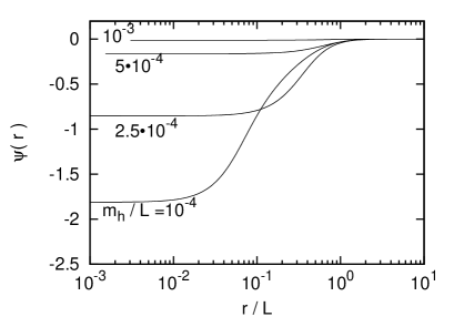
(b) Black hole $+$ CFT

Figure 8: The metric function $\psi(r)$ for CFT stars (left panel) and for quantum black holes (right panel) for various central densities and black hole masses, respectively. We set $\ell/L=10^{-5}$.

(a) CFT star

(b) Black hole $+$ CFT

Figure 9: Plot for the metric function $m(r)$ in the same way as in Fig. 8.

It is easy to see that the metric functions are almost the same for the star sequence in the large central density limit and for the black hole sequence in the small size limit. Let us focus on, for example, the curves for $\rho_{\rm c}L^{2}=10^{2}$ in the left panel and $m_{\rm h}/L=10^{-4}$ in the right panel. First, for a small radius ($r/L\lesssim 10^{-2}$ for $\rho_{\rm c}L^{2}=10^{2}$ and $m_{\rm h}/L=10^{-4}$), there is a constant density core described by

$$\psi(r)\sim\text{const}~{},$$ (47)

and

$$\frac{m(r)}{L}\sim\text{const}\times\left(\frac{r}{L}\right)^{3}.$$ (48)

Here the constants are determined by the central density or the black hole mass. This region is followed by the intermediate region ($10^{-2}\lesssim r/L\lesssim 1$). The behavior in this region is approximately obtained by solving Eqs. (23) and (25) for $r/L\ll 1$, assuming power law solutions for $m$ and $\rho$. With the aid of Eqs. (22), (23) and (24), we obtain

$$\frac{m(r)}{L}\sim\frac{3}{14}\left(\frac{r}{L}\right),$$ (49)

and

$$\psi(r)\sim\frac{1}{2}\ln\left(\frac{r}{L}\right)~{}.$$ (50)

For stars with large central density and for black holes with small mass, $\psi(r)$ takes a large negative value for a small $r$, which means a large red shift factor. The growth of red shift factor compensates the usual growth of black hole temperature in the small black hole limit, and explains the convergence of global temperature of the system. We also mention that in the black hole case the back reaction effects are small for $\bar{r}_{\rm h}\gtrsim(\ell^{2}L^{3})^{1/5}$. In this case $m(r)$ takes an almost constant (not small) value all over the spacetime (dotted lines in the right panel of Fig. 9).

V AdS/CFT interpretation

In this section we will discuss the implications of our calculations for black hole solutions in the KR model based on the AdS/CFT correspondence Gubser2 ; Hawking ; tanaka . When we discuss the AdS/CFT correspondence in the KR model, our asymptotically AdS brane does not throughly surround the five-dimensional bulk space. Therefore, in addition to the CFT considered so far (CFT1), we need to include the contributions from another CFT residing on the boundary that limits the other side of the bulk (CFT2) KR2 . As long as thermal equilibrium state is concerned, we have to relate the temperature of CFT2 to that of CFT1. For convenience, we introduce a second brane at a finite but large distance from the first brane. We calculate first the entropy of CFT2 on this second brane and then send the brane separation to infinity. The line element of four-dimensional metric induced on the second brane is approximated by the pure AdS metric:

$$ds^{2}=-f(r_{2})dt_{2}^{2}+f(r_{2})^{-1}dr_{2}^{2}+r_{2}^{2}d\Omega^{2}~{},$$ (51)

where $t_{2}$ and $r_{2}$, respectively, are time and radial coordinates on the second brane, $f(r_{2})\equiv 1+r_{2}^{2}/L_{2}^{2}$, and $L_{2}$ is the AdS curvature length on the second brane. The infinitesimal proper time interval for a static observer in these coordinates is $f(r_{2})^{1/2}dt_{2}$. On the other hand, this brane can be embedded in the five-dimensional bulk, which behaves as (6) in the asymptotic region. In the coordinates of Eq. (6) the second brane is located at $y=y_{2}$ approximately. The proper time interval in these coordinates is described by $\ell\cosh(y_{2}/\ell)\,(1+\bar{r}^{2})^{1/2}d\bar{t}$. Thus, the ratio between these two time coordinates is

$$dt_{2}/d\bar{t}=dr_{2}/d\bar{r}=\ell\cosh(y_{2}/\ell)=L_{2}~{}.$$ (52)

As for the first brane, a parallel discussion applies as long as a large radius limit is concerned. The induced metric on the first brane is also asymptotically AdS, and the location of the brane is also specified by a $y$-constant surface there. Thus, we find $dt_{2}/dt=L_{2}/L$. Therefore, when thermal equilibrium is realized in the five-dimensional picture, the relation between the temperatures of CFT1 and CFT2 is given by

$$TL=T_{2}L_{2}~{}.$$ (53)

By using the radiation fluid approximation, the entropy of CFT2 can be estimated as

$$S^{CFT2} = \int^{\infty}_{0}4\pi r^{2}\sqrt{g_{rr}}\,s\,dr={\pi^{5}\over 2G_{4}}T^{3}L^{3}l^{2},$$ (54)

where $s=(4/3)(\pi^{2}/30)g_{\rm eff}(T_{2}/\alpha)^{3}$ is the radiation fluid entropy density with $g_{\rm eff}$ given in Eq. (16). Since the entropy estimated in Eq. (54) is independent of the position of the second brane where the CFT2 lives, we send the second brane to the bulk boundary by taking the limit $y_{2}\to\infty$.

Now, let us consider brane-localized black holes which should correspond to four-dimensional asymptotically AdS quantum black holes. The AdS/CFT correspondence indicates that the micro-canonical stability in the four-dimensional CFT picture should correspond to the dynamical stability in the five-dimensional picture. (Notice that there is no reservoir of energy in the present system.) Hence, the previous discussion should be slightly modified by taking into account the contribution from CFT2. Estimating the mass for the CFT2 taking into account a redshift factor, the total mass of the system will be given by

$$M_{\rm tot}=M^{CFT1}\Bigl{(}\bar{r}_{\rm h},\ell,L\Bigr{)}+{3\pi^{5}\over 8G_{4}}T^{4}\Bigl{(}\bar{r}_{\rm h},\ell,L\Bigr{)}L^{3}\ell^{2},$$ (55)

(56)

where the first term represents what we evaluated numerically in the preceding section and the second term is the contribution from CFT2. A micro-canonical stable-unstable transition takes place at $\bar{r}_{\rm h}=0.38\cdot(\ell^{2}L^{3})^{1/5}$, where $M_{\rm tot}$ above is minimized. Therefore the brane-localized black holes are expected to be stable (unstable) when the circumferential radius of the brane cross-section of the horizon is larger (smaller) than the above critical value.

We can also discuss the possible shape of the corresponding five-dimensional solution. In the KR model, there is a black string solution, and its brane induced geometry is exactly Schwarzschild AdS. Although this solution does not satisfy the boundary condition that the metric should get close to the five-dimensional pure AdS at $y\to\infty$, we expect that, when the induced geometry of a brane-localized black hole is close to Schwarzschild AdS, the bulk geometry is also close to a black string solution. As we showed in the preceding section, this is the case when the four-dimensional horizon radius is larger than $(\ell^{2}L^{3})^{1/5}$. In this case the metric function $m(r)$ is almost constant and $\psi(r)\sim 0$ for any $r$. (see Figs. 8 and 9). The AdS/CFT correspondence suggests that large black holes should look like black strings in the five-dimensional picture, but there is small deviation from the Schwarzschild AdS. We expect that this small deviation is due to the truncation of the horizon of the “black string” at a finite distance far from the brane, having a cap there. Roughly speaking, the cap will be formed near the throat corresponding to $y=0$. In contrast, when $\bar{r}_{\rm h}\lesssim(\ell^{2}L^{3})^{1/5}$, the behavior of $m(r)$ and $\psi(r)$ is clearly different from the Schwarzschild AdS case. This indicates that the five-dimensional bulk black hole dual to a four-dimensional unstable black hole is not like a black string.

We can also estimate the expected size of the black hole in the five-dimensional picture since the entropy is related to the five-dimensional area of black hole horizon $A_{5}$ by

$$S=\frac{A_{5}}{4G_{5}}~{}.$$ (57)

We may define the corresponding five-dimensional horizon radius by

$$r_{\rm h}\equiv\left({A_{5}\over 2\cdot 2\pi^{2}}\right)^{1/3}~{},$$ (58)

where the factor $2$ represents the presence of two floating black holes (one for each side of the bulk interrupted by the brane). The total entropy and hence the size of bulk floating black holes are almost constant in the course of the transition (see Fig. 6). For example, the horizon radius of the five-dimensional black hole, $r_{\rm h}$, at the stability changing point is estimated as

$$r_{\rm h}=0.7\cdot(\ell^{3}L^{2})^{1/5},$$ (59)

from $\ell^{-4/5}L^{-6/5}G_{4}S_{\rm tot}=3.4$ at $\bar{r}_{\rm h}=0.38\cdot(l^{2}L^{3})^{1/5}$, where

$$S_{\rm tot}=S^{CFT1}\Bigl{(}\bar{r}_{\rm h},\ell,L\Bigr{)}+{\pi^{5}\over 2G_{4}}T^{3}\Bigl{(}\bar{r}_{\rm h},\ell,L\Bigr{)}L^{3}\ell^{2}.$$ (60)

(61)

Again, the first term represents what we evaluated numerically in the preceding section and the second term is the contribution from CFT2.

Let us now move on to the transition between the sequences of floating black holes and brane-localized black holes. Corresponding to this transition, in the four-dimensional picture, we have confirmed that there is a transition between CFT stars and quantum black holes. According to the results of our calculation, the transition occurs at

$$\ell^{1/2}L^{1/2}T = 0.21,$$

$$\ell^{-1/2}L^{-3/2}G_{4}S_{\rm tot} = 2.0+1.4=3.4.$$ (62)

Here, $2.0$ comes from CFT1 and $1.4$ from CFT2. These critical values are independent of the ratio $\ell/L$. From the entropy, the horizon radius of the five-dimensional black hole just touching the brane is estimated as

$$r_{\rm h}=0.7\cdot(lL)^{1/2}.$$ (63)

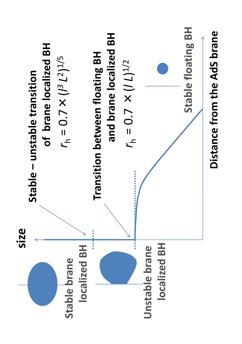
Figure 10: Phase diagram of BH solutions in the KR model.

As we can see from Figs. 8 and 9, the geometry of a star configuration in the large central density limit is very similar to that of a small black hole. This indicates that the five-dimensional geometry is also similar between the bulk floating black holes just before touching the brane and the brane-localized black holes just after touching. The expected phase diagram of black hole solutions in the KR model is illustrated in Fig. 10.

Before closing this section, we would like to mention the screening effect. As we have seen, if we use the Page’s approximation instead of our more crude radiation fluid approximation, the mass varies logarithmically in $r$ at infinity. In five-dimensional picture this phenomena can be understood as the leakage of gravitons from the brane on the CFT1 side because massless gravitons in the four-dimensional sense, which mediate the mass information to the infinity, are localized on the CFT2 side. Then, at a large distance the leaked energy should be observed as the energy on the CFT2 side. In the four-dimensional CFT language this transmutation of energy from CFT1 to CFT2 can be correctly described only when the interaction between CFT1 and CFT2 is treated appropriately. However, in the fluid approximation we treated CFT1 and CFT2 as completely independent components except for tuning the temperature. In such a treatment the energy transfer from CFT1 to CFT2 is not taken into account. Therefore, when we identify the mass, we do not have to worry about the screening effect in this approximation.

VI Summary

We analyzed asymptotically AdS configurations with and without event horizon in thermal equilibrium including the quantum back reaction due to CFT by using radiation fluid approximation with the aim to clarify the phase diagram structure of black objects in the KR model. We referred to the configurations with and without a horizon as CFT stars and quantum black holes, respectively. We have confirmed that the radiation fluid approximation is good when typical length scales like the horizon radius $\bar{r}_{\rm h}$ of the black hole are all larger than the bulk curvature scale $\ell$, in which the AdS/CFT correspondence is expected to be valid. We calculated the metric and the thermodynamic quantities and found that: (i) the sequence of solutions of CFT stars is smoothly connected to the sequence of quantum black holes in the limit of infinite central density, (ii) the thermodynamically stable-unstable transition in the sequence of quantum black holes occurs when the horizon radius $\bar{r}_{\rm h}$ is about $(\ell^{2}L^{3})^{1/5}$, (iii) because of the back reaction effects, the temperature of the system converges to $\approx 0.21\cdot(\ell L)^{-1/2}$ in the limit $\bar{r}_{\rm h}\rightarrow 0$, (iv) for $\bar{r}_{\rm h}\gtrsim(\ell^{2}L^{3})^{1/5}$, back reaction effects are negligible and the space-time is approximately given by Schwarzschild AdS.

We also discussed the implications of our calculations for black hole solutions in the KR model based on the AdS/CFT correspondence. We claimed that (i) there are stability changing points along the sequence of brane-localized black hole solutions. The first transition corresponding to the minimum total mass of the system occurs when the five-dimensional horizon radius is $\approx 0.7\cdot(\ell^{3}L^{2})^{1/5}$; (ii) the sequence of bulk floating black holes leads to the sequence of brane-localized black holes and this transition between these two sequences occurs when the black hole temperature is $\approx 0.21\cdot(\ell L)^{-1/2}$ and the five-dimensional black hole horizon radius is $\approx 0.7\cdot(lL)^{1/2}$.

VII Acknowledgements

This work is supported by the JSPS through Grants Nos. 19540285, 19GS0219, 2056381, 20740133, 21244033. We also acknowledge the support of the Global COE Program “The Next Generation of Physics, Spun from Universality and Emergence” from the Ministry of Education, Culture, Sports, Science and Technology (MEXT) of Japan is kindly acknowledged.

References

- (1) J. M. Maldacena, Adv. Theor. Math. Phys. 2 231 (1998).
- (2) E. Witten, Adv. Theor. Math. Phys. 2 253 (1998).
- (3) S. S. Gubser, I. R. Klebanov, A. M. Polyakov, Phys. Lett. B 428 105114 (1998).
- (4) L. Randall, R. Sundrum, Phys. Rev. Lett. 83 4690 (1999).
- (5) J. Garriga, T. Tanaka, Phys. Rev. Lett. 84, 2778 (2008).
- (6) S. S. Gubser, Phys. Rev. D 63, 084017 (2001) [arXiv:hep-th/9912001].
- (7) S. W. Hawking, T. Hertog, H. S. Reall, Phys. Rev. D 62 043501 (2000).
- (8) T, Tanaka,arXiv:gr-qc/0402068
- (9) L. Grisa, O. Pujolas, J. High Energy Phys. 0806 059 (2008)
- (10) M. J. Duff, J. T. Liu, Phys. Rev. Lett. 85 2052 (2000).
- (11) T. Tanaka, Prog. Theor. Phys. Suppl. 148 307 (2003).
- (12) T. Shiromizu, D. Ida, Phys. Rev. D 64 044015 (2001).
- (13) J. Garriga, M. Sasaki, Phys. Rev. D 62 043523 (2000).
- (14) H. Kudoh, T. Tanaka, N. Nakamura, Phys. Rev. D 68 024035 (2003).
- (15) H. Yoshino, J. High Energy Phys. 01 068 (2009).
- (16) R. Emparan, A. Fabbri, N. Kaloper, J. High Energy Phys. 0208 043 (2002).
- (17) A. Karch, L. Randall, J. High Energy Phys. 05 008 (2001).
- (18) T. Tanaka, Prog. Theor. Phys. Suppl. 121 1133 (2009).
- (19) A. Flachi, T. Tanaka, Phys. Rev. D 78, 064011 (2008).
- (20) D. N. Page, Phys. Rev. D 25 1499-1509 (1982).
- (21) A. Karch, L. Randall, Phys. Rev. Lett. 87 061601 (2001).
- (22) R. Gregory, S. F. Ross, R. Zegers, J. High Energy Phys. 09, 029 (2008).
- (23) P. R. Anderson, W. A. Hiscock, D. A. Samuel, Phys. Rev. D 51 4337 (1995).
- (24) M. Porrati, J. High Energy Phys. 0204, 058 (2002).
- (25) M. J. Duff, J. T. Liu and H. Sati, Phys. Rev. D 69 085012 (2004).
- (26) S. S. Gubser, I. R. Klebanov, A. W. Peet, Phys. Rev. D 54 3915 (1996).
- (27) D. N. Page, and K. C. Phillips, Gen. Rel. Grav. 17 1029 (1985).