Sparse regular random graphs: Spectral density and eigenvectors

Abstract

We examine the empirical distribution of the eigenvalues and the eigenvectors of adjacency matrices of sparse regular random graphs. We find that when the degree sequence of the graph slowly increases to infinity with the number of vertices, the empirical spectral distribution converges to the semicircle law. Moreover, we prove concentration estimates on the number of eigenvalues over progressively smaller intervals. We also show that, with high probability, all the eigenvectors are delocalized.

and

t2Supported by NSF CAREER Award DMS-08-47661. t3Supported in part by NSF Grant DMS-10-07563.

1 Introduction

Consider the uniform distribution over the space of all labeled simple graphs on $n$ vertices where every vertex has degree $d$. We denote a graph randomly selected from this distribution by $G(n,d)$; the vertices of $G(n,d)$ will always be labeled by $\{1,2,\ldots,n\}$.

Now, consider a sequence of such random graphs $\{G(n,d_{n}),n\in\mathbb{N}\}$ which are $d_{n}$-regular of order $n$. We assume $d_{n}$ to be slowly growing with $n$ in a manner which will be made more precise later. Consider the adjacency matrix $A_{n}$ of $G(n,d_{n})$; the $(i,j)$th element of $A_{n}$ is one or zero depending on whether there is an edge between vertices $i$ and $j$ in the graph $G(n,d_{n})$. The random matrix $A_{n}$ is always symmetric, and it has $n$ real eigenvalues (perhaps not all distinct) and corresponding real eigenspaces. Under appropriate conditions on the growth of the sequence $d_{n}$, we study the following phenomena as $n$ tends to infinity: [(iii)]

Global semicircle law. We prove the convergence of the empirical spectral distribution (ESD) of the scaled adjacency matrix to the probability measure on $[-2,2]$ with density

$$f_{\mathrm{sc}}(x)=\frac{1}{2\pi}\sqrt{4-x^{2}},\qquad-2<x<2.$$ (1)

Local semicircle law (a.k.a. the semicircle law on short scales). We obtain concentration estimates of the deviation of the number of eigenvalues $\mathcal{N}_{I}$ that lie in a small interval $I$ from its predicted number $n\int_{I}f_{\mathrm{sc}}(x)\,dx$. The size of $I$ will be taken to be vanishing at an appropriate rate with increasing $n$.

Delocalization of eigenvector coordinates. We obtain probability estimates of the event that, for some eigenvector, a few of the coordinates are significantly larger in magnitude than the rest.

These problems connect two areas of study: Wigner random matrices and spectra of sparse random graphs; since we have already mentioned the latter, we will now talk about the former.

In the last couple of decades there has been an enormous amount of activity in the study of universal properties of random matrices, inspired by their connection to (universal) physical systems. The literature on universality studies in random matrices is vast; we mention here only a few references and ask the reader to look to them for further ones.

For an introduction and motivation to the subject, we recommend Deift’s ICM address deift06a . Of particular interest are the Wigner matrices (see Bai baiconv , Soshnikov soshuniv , Bai and Yao baiyao05 , Khorunzhy, Khoruzhenko and Pastur khokhopastur , Guionnet and Zeitouni guionnetzeitouni , Ben Arous and Peche benarouspeche , Tao and Vu taovu , taovu2 ). Deift and Goiev deiftgioev looked at different potential functions on symmetric, Hermitian and self-dual matrices; Baik and Suidan explored connections to percolation baiksuidan05 and random walks baiksuidan07 ; $\beta$-generalizations of the classical ensembles and universal properties thereof have been explored in Forrester and Baker Forresterpoly , Johansson johanssoncltherm , Dumitriu and Edelman dumitriu06 . Recently, more sophisticated probability tools have been generalized and applied to random matrix theory (e.g., the Lindeberg Principle, by Chatterjee chatterjee and Tao and Vu taovu , taovu2 ).

Most of the focus in universality research has been on proving, under progressively weaker assumptions on the entry distribution, the following:

• convergence of the ESD to the semicircle or Marčenko–Pastur laws and establishing rates of convergence in various ways (large deviations, concentration estimates, central limit theorems). For a comprehensive treatment of the subject, see the books by Bai and Silverstein baisil and by Anderson, Guionnet and Zeitouni agzbook ;

• fluctuations of the spectrum at the edge (the famous Tracy–Widom laws twl , twuniv1 , twuniv2 ) for general Wigner matrices, settled by Tao and Vu taovu2 and Erdős et al. ERSTVY ;

• universality of correlation functions in the bulk, under various assumptions (Tao and Vu taovu , Erdős et al. ERSTVY , Erdős et al. eprsy , Erdős, Yau and Yin eyy );

• partial or complete delocalization of the eigenvectors (by Erdős, Schlein and Yau esy1 , esy2 and Tao and Vu taovu , taovu2 ).

The aim of said research has been to show that the spectral statistics agree in the large $n$ limit to the spectral statistics of the Gaussian Orthogonal Ensemble (GOE) and the Gaussian Unitary Ensemble (GUE), depending on whether the matrices are real symmetric/positive-definite, or complex Hermitian/positive-definite. The Gaussian and Wishart ensembles are some of the most studied and best understood random matrix models; for an easy introduction to classical random matrix theory, see the books by Mehta mehtabook and Muirhead muirhead82a .

Parallel to these developments, in combinatorics and discrete mathematics, there has always been an interest in studying spectral properties of deterministic and random graphs. There are two matrices of interest in spectral graph theory: the adjacency (sometimes called the incidence) matrix, which we already defined, and the Laplacian matrix. These matrices are the same for regular graphs (although, in general, they can be quite different), and the spectrum of the graph is the spectrum of the matrix.

Among the properties of random graphs that have been the focus of intense research are connectivity, phase transitions and the limiting spectral distribution of random graphs, including trees (McKay mckay81 , Feige and Ofek feigeofek05 , Mirlin and Fyodorov mirlinfyod91 , Bauer and Golinelli bauergolinelli01 , Semerjian and Gugliandolo semerjian02 , Bordenave and Lelarge bordlelarge , Bhamidi, Evans and Sen bhamidievanssen ). Other properties include concentration of eigenvalues (Krivelevich and Sudakov krivsudakov03 , Alon, Krivelevich and Vu alonkrivvu ), the spectral gap (Fűredi and Komlós furedikomlos , Friedman friedmane2 and Friedman and Alon friedmanalon , Broder and Shamir brodershamir ).

Another area of recent interest is the study of quasi-random graphs and expanders. These are nonrandom graphs which display properties one expects to hold with high-probability for certain classes of random graph models. For example, expanders are sparse graphs that have high connectivity properties (e.g., a large spectral gap). These graphs are often regular (e.g., the famous Ramanujan graph, described in the seminal articles by Lubotzky, Phillips and Sarnak LPS and Morgenstern morgenstern ). Random $d$-regular graphs display the same connectivity properties with very high probability, when $d$ is kept fixed and the order is large; this is in essence the Alon conjecture, recently settled by Friedman friedmanalon . Thus a study of random regular graphs suggests possible properties of (deterministic) expanders.

It is easy for a probability audience to appreciate the importance of studying eigenvalues of the graph (e.g., the spectral gap which determines the mixing properties of a random walk), but eigenvectors of graphs are equally important, especially since they are the solutions of various combinatorial optimization problems. Traditionally, there has been much less work on computing the actual graph eigenvector distributions, with the notable and recent exception of Wishart-like sample covariance matrices (see Bai, Miao and Pan buymeapan ). Thus, developments in examining properties of the eigenvectors of large random graphs (as in Friedman friedmannodal and Dekel, Lee and Linial dekelleelinial ) are relatively new, and motivated by the applications of eigenvectors to engineering and computer science. Such applications include the Google page-rank algorithm pagerank , the Shi–Malik algorithm shimalik00 , the Meila–Shi algorithm meilashi and other spectral clustering techniques and related segmentation problems (Weiss weiss99 , Pothen, Simon and Liou pothensimonliou , etc.).

It is probably clear by now that the two fields of research that we have very briefly sketched here (universality studies in random matrix theory and spectra of random graphs) are vast and, by examining the two lists of important problems we have outlined, one can see that there is a certain amount of overlap. Naturally, this lead to a few papers where the two fields have intersected, despite differences in both the goals and the methodology of each.

A famous such example is McKay’s derivation of the limiting empirical spectrum of random $d$-regular graphs on $n$ vertices, as $d$ is fixed and $n$ grows to infinity mckay81 . In that case, the empirical spectral distribution converges in probability to what is known as the McKay (or Kesten–McKay) law, which has a density

$$f_{d}(x)=\frac{d\sqrt{4(d-1)-x^{2}}}{2\pi(d^{2}-x^{2})},\qquad-2\sqrt{d-1}\leq x\leq 2\sqrt{d-1}.$$ (2)

This density had appeared earlier in Kesten’s work on random walks on groups kesten . It can be easily verified that as $d$ grows to infinity, if we normalize the variable $x$ in the above by $\sqrt{d-1}$, the resulting density converges to the semicircle law on $[-2,2]$.

This naturally raised the question of whether the study of “universal” properties could be pushed into the domain of regular random graphs with increasing degree. The rate of growth of the degree sequence plays an important role, since at both extremes ($d$ fixed and $d=n-1$) the ESDs do not converge to the semicircle law.

The answer to this question turns out to be difficult. There are a number of major obstacles to developing an applicable universality theory in the spirit of Wigner random matrices to adjacency matrices of random graphs, which are non-Wigner: these matrices are sparse and the entries are not independently distributed.

To see how sparsity affects concentration, consider the question of proper scaling of the adjacency matrix $A_{n}$. In the Wigner case, the scaling factor is clearly $1/\sqrt{n}$, which puts all of the eigenvalues in $[-2-\varepsilon,2+\varepsilon]$, for any positive $\varepsilon$, with very high probability for a sufficiently large $n$. One might be tempted then to believe that the proper scaling for adjacency matrices is $1/\sqrt{d_{n}}$, as this achieves the same kind of finite row-variance as $1/\sqrt{n}$ does in the Wigner case. Unfortunately, it is not known if this scaling will place all the eigenvalues (except the first) in a compact interval, as $d_{n}\rightarrow\infty$.

For the regime when $d$ is fixed, the Alon conjecture states that the second largest eigenvalue (in absolute value) $\lambda_{2}$ has an upper bound $|\lambda_{2}|\leq 2\sqrt{d-1}+\varepsilon$, with very high probability. The well-known lower bound holds for every $d$-regular graph and we cite it from Friedman friedmane2 : $|\lambda_{2}|\geq 2\sqrt{d-1}+O({\log d}/{\log n})$. Unfortunately, when $d$ grows with $n$, the upper bound is not known to hold outside of a narrow growth regime. Khorunzhy khorunzhy01 has shown that, for a random matrix model similar to the adjacency matrix of the Erdős–Renýi random graph on $n$ vertices with an expected degree $d_{n}\gg\log n$, with probability one, the spectral norm of the adjacency matrix grows faster than $\sqrt{d_{n}}$. Although this does not necessarily affect convergence of the ESD to the semicircle law, it eliminates the possibility of containing all the eigenvalues of the rescaled centralized adjacency matrix within any compact interval.

Our results investigate the extent to which universality can be extended to the slowly growing $d_{n}$ case. Our first result is Theorem 1 stated below.

Theorem 1

Let $d_{n}$ satisfy the asymptotic condition

$$\lim_{n\rightarrow\infty}d_{n}=\infty,\qquad d_{n}-1=n^{\varepsilon_{n}}\qquad\mbox{for some }\varepsilon_{n}=o(1).$$ (3)

Then the ESD of the matrix $(d_{n}-1)^{-1/2}A_{n}$, where $A_{n}$ denotes the adjacency matrix of $G_{n}$, converges in distribution to the semicircle law on $[-2,2]$ which has a density

$$f_{\mathrm{sc}}(x):=\frac{1}{2\pi}\sqrt{4-x^{2}},\qquad-2<x<2.$$ (4)

The condition on $d_{n}$, for example, includes the logarithmic regime, $d_{n}=(\log n)^{\gamma}$ for any positive $\gamma$; in which case we can define $\varepsilon_{n}$ as $\gamma\log\log n/\log n$.

Our proof of this result (and the following ones) depends crucially on two facts: [(ii)]

the “locally tree-like” property, which states that with high probability, most vertices in a random regular graph will have a (increasingly larger) neighborhood which is free of any cycles, and

the fact that $d_{n}$ grows to infinity, which smooths out irregularities as $n$ tends to infinity.

Our second result is arguably the most important one in this paper.

Theorem 2

Fix $\delta>0$. Let $d_{n}=(\log n)^{\gamma}$, where $\gamma>0$. Let $\eta_{n}=(r_{n}-r_{n}^{-1})/2$ where $r_{n}=\exp(d_{n}^{-\alpha})$ for some $0<\alpha<\min(1,1/\gamma)$. Then there exists an $N$ large enough such that for all $n\geq N$, for any interval $I\subset\mathbb{R}$ of length $|I|\geq\max\{2\eta_{n},\eta_{n}/(-\delta\log\delta)\}$,

$$\biggl{|}\mathcal{N}_{I}-n\int_{I}f_{\mathrm{sc}}(x)\,dx\biggr{|}<\delta n|I|$$

with probability at least $1-o(1/n)$. Here $\mathcal{N}_{I}$ is the number of eigenvalues of $\frac{1}{\sqrt{d_{n}-1}}A_{n}$ in the interval $I$, and $f_{\mathrm{sc}}$ refers to the density of the semicircle law as in (1).

Remark 1.

Note that the shortest length of the interval $I$ that our methods can narrow down to is of length $\eta_{n}$, which is roughly about $1/\log n$, if $d_{n}\gg\log n$, and $1/d_{n}$, if $d_{n}\ll\log n$. For Wigner matrices a far shorter scale can be achieved (effectively poly-log over $n$ in esy1 ). Such sharp estimates are not to be expected in the graph case, and this again is a consequence of sparsity and lack of concentration estimates.

Remark 2.

A close examination of the proof of Theorem 2 reveals that it can be extended to any deterministic sequence of regular graphs of increasing size and degree, as long as the “locally tree-like” property holds at “most” vertices.

Remark 3.

Since the submission of this paper, significant progress has been made in proving the local semicircle law for random regular graphs in any kind of growth regime for $d_{n}$ (see Tran, Vu and Wang TVW ). Their methods rely on proving the local semicircle law first for Erdős–Rényi graphs with suitable parameters, and then using a result by McKay and Wormald MW about the probability that an Erdős–Rényi graph is regular. Their result subsumes ours (in the sense that the lower bound on the length of the interval $I$ is smaller) for the case when $d_{n}=\Omega((\log n)^{10})$; when $d_{n}=o((\log n)^{10})$, our result is slightly stronger in the same sense.

Although these results are similar up to a point to the Wigner matrix results, our methodology is essentially different. Due to sparsity and lack of concentration, we had to adapt a more combinatorial set of tools (in particular, the tree approximation) as well as tools from linear algebra to the Stieltjes transform approach used in esy1 and taovu .

Several recent articles have done extensive simulations on eigenvalues and eigenvectors of random graphs, with surprising conclusions. For example, Jakobson et al. simeval carries out a numerical study of fluctuations in the spectrum of regular graphs. Their experiments indicate that the level spacing distribution of a generic $k$-regular graph approaches that of the GOE as we increase the number of vertices. On the eigenvector front, in the article simevec by Elon, the author attempts to characterize the structure of the eigenvectors by suggesting (with numerical observations) that all, except the first, follow approximately a Gaussian distribution. Additionally, the local covariance structure has been conjectured to be given by explicit functions of the Chebyshev polynomials of the second kind. In particular, if two vertices on the graph are at a distance $k$ from each other, it is conjectured that the covariance between the coordinates of any eigenvector at the two vertices decays exponentially in $k$.

All this empirical data points to universality properties of the adjacency matrices of large, sparse regular graphs; we took here a first step toward proving them.

If the eigenvectors are indeed uniformly distributed over the sphere then they must (with high probability) satisfy delocalization. We give upper bounds on the probability of this phenomenon.

We use the following definition of delocalization, similar to the one used in esy1 .

Definition 1.

Let $T$ be a subset of $\{1,2,\ldots,n\}$ of size $L\geq 1$. Let $\delta>0$ be some fixed number. We say that a vector $v=(v(1),\ldots,v(n))\in\mathbb{R}^{n}$ with $\mathbb{L}^{2}$ norm $\|v\|_{2}=1$ exhibits $(T,\delta)$ localization if

$$\|v\mid_{T}\|_{2}^{2}=\sum_{j\in T}|v(j)|^{2}\geq 1-\delta.$$

The vector $v$ is said to be $(L,\delta)$ localized there exists some set $T\subset\{1,2,\ldots,n\}$ such that $|T|=L$ such that $v$ is $(T,\delta)$ localized.

Below is our result on eigenvector delocalization.

Theorem 3

Assume the set-up of Theorem 2. Fix $\delta>0$.

[(ii)]

Let $T_{n}\subseteq\{1,2,\ldots,n\}$ be a deterministic sequence of sets of size $L_{n}=o(\eta_{n}^{-1})$. Let $\Omega_{1}(n)$ be the event that some normalized eigenvector of the matrix $A_{n}$ is $(T_{n},\delta)$ localized. Then, for all sufficiently large $n$,

$$P((\Omega_{1}(n))^{c})\geq e^{-L_{n}\eta_{n}/d_{n}}\biggl{(}1-o\biggl{(}\frac{1}{d_{n}}\biggr{)}\biggr{)}=1-o\biggl{(}\frac{1}{d_{n}}\biggr{)}.$$

Define the sequence

$$\zeta_{n}=\frac{1}{4}\frac{\log n}{\log(d_{n}-1)}-4,\qquad n\geq 2.$$

Consider the (random) subset $J(n)$ of all vertices in the graph whose $\zeta_{n}$-neighborhood is free of cycles. Then,

$$P\biggl{(}\frac{|J(n)|}{n}\geq 1-\frac{\eta_{n}}{d_{n}}\biggr{)}=1-o\biggl{(}\frac{1}{n}\biggr{)}.$$

Moreover, there exists an $n$ large enough such that the event that $T_{n}\subset J(n)$ and some normalized eigenvector is $(T_{n},\delta)$ has probability zero.

Remark 4.

More progress has been made on the eigenvector delocalization front since the submission of this paper. In their paper TVW , the authors prove that the $\ell^{\infty}$ norms of all eigenvectors are $o(1)$, regardless of the regime of growth of $d_{n}$. Very recently, Erdős et al. posted a paper EKYY proving the local semicircle law for Erdős–Rényi graphs with $pn=\Omega(\log n)$ up to a spectral window (an interval $I$) of size larger than $1/n$; from this, they could deduce that the eigenvectors of such Erdős–Rényi graphs are completely delocalized, that is, that the $\ell^{\infty}$ norms of the normalized (unit) eigenvectors are at most of order $1/\sqrt{N}$ with high probability. It would be interesting to see if the methods of TVW (of deducing results for random regular graphs from the same results for Erdős–Rényi) can be combined with the theorems of EKYY to obtain complete eigenvector delocalization (and, potentially, a much smaller spectral window) for random regular graphs with $d_{n}=\Omega(\log n)$.

The bounds in Theorem 3 are not sharp. There are severe technical obstacles in producing sharp bounds by adapting the strategy of Wigner matrices. One such example is eigenvalue collision, that is, the event that $A_{n}$ does not have $n$ distinct eigenvalues. Since $A_{n}$ has discrete entries, this event has a positive probability. However, to the best of our knowledge, no good bound on this probability is known.

The paper is organized as follows. In Section 2 we prove the global convergence to the semicircle law (Theorem 1). This is followed by the proof of the local semicircle law (Theorem 2) in Section 3. The eigenvector delocalization is proved in Section 4. Finally, the Appendix contains an exact calculation of eigenvalues and eigenvectors for the random regular (finite) tree, defined in Section 2.

2 Global convergence to the semi-circle law

Recall that $G_{n}=G(n,d_{n})$ denotes a random $d_{n}$-regular graph on $n$ vertices whose adjacency matrix is $A_{n}$. Recall that $d_{n}$ satisfies the asymptotic condition

$$\lim_{n\rightarrow\infty}d_{n}=\infty,\qquad d_{n}-1=n^{\varepsilon_{n}}\qquad\mbox{for some }\varepsilon_{n}=o(1).$$ (5)

We prove here Theorem 1, namely, that the empirical spectral distribution (ESD) of the adjacency matrix $A_{n}$ converges in probability to the semicircle law on $[-2,2]$ which we recall from (4).

Our main instrument is to use the moment method. Our arguments depend crucially on the following local approximation of $G_{n}$ by a rooted tree. Consider the deterministic rooted tree $S_{n}$, which is the infinite regular tree of degree $d_{n}$ with a distinguished vertex marked as the root. For a graph $G$ whose every edge is taken to have unit length, consider the induced metric structure on $G$. We define the $r$-neighborhood of the vertex $i$, to be the subgraph of $G$ whose vertices are at a distance at most $r$ from $i$, and whose edges are all the edges between those vertices. The following lemma makes precise the idea that, except for a vanishing proportion of the vertices, the $r$-neighborhood of any vertex is isomorphic to the corresponding neighborhood of the root in the tree $S_{n}$.

Recall that a cycle is a sequence of vertices $\{i_{1},\ldots,i_{k}\}$ of a graph such that $i_{1}=i_{k}$, there is no other repeated vertex, and there is an edge between every successive $i_{j}$ and $i_{j+1}$. The length of the cycle is the number of vertices except the initial one. A cycle of length $k$ will be called a $k$-cycle. Finally, a cycle-free or acyclic graph is a tree.

Lemma 4

Fix a positive integer $r$. Let $\tau(n)$ be the subset of vertices of $G_{n}$ which have no cycles in their $r$-neighborhoods, and let $|\tau(n)|$ denote the size of $\tau(n)$. Then, under the assumptions of (5), we have

$$P\biggl{(}1-\frac{|\tau(n)|}{n}>n^{-1/4}\biggr{)}=o(n^{-5/4}).$$

We use the estimates of McKay, Wormald and Wysocka mww04 on the Poisson approximation to the number of short cycles in regular graphs. Let $g(n)$ be a sequence such that

$$g(n)\geq 3\quad\mbox{and}\quad(d_{n}-1)^{2g(n)-1}=o(n).$$ (6)

For any $s\leq g$, let $M_{s}$ denote the number of cycles of length $s$ in the graph $G_{n}$. It has been shown in mww04 that $M_{s}$ is approximately distributed as a Poisson random variable and

$$E(M_{s}) = \mu_{s}\bigl{(}1+O\bigl{(}s(s+d)/n\bigr{)}\bigr{)}\qquad\mbox{where }\mu_{s}=\frac{(d-1)^{s}}{2s}\quad\mbox{and}$$

$$\operatorname{Var}(M_{s}) = \mu_{s}+O\bigl{(}s(s+d)/n\bigr{)}\mu_{s}^{2}.$$

Consider now the growth of the degree sequence as in (5). If we choose $g(n)$ such that $2g(n)-1=1/\sqrt{\varepsilon_{n}}$, it will satisfy

$$(d_{n}-1)^{2g(n)-1}=n^{\sqrt{\varepsilon_{n}}}=o(n).$$

Additionally $g(n)$ grows to infinity with $n$, since $\varepsilon(n)=o(1)$.

Consider an $s$-cycle for some $s\leq g(n)$. It has exactly $s$-vertices. Now, the number of vertices whose $r$ neighborhoods fail to be acyclic because of this $s$-cycle are precisely those vertices which are at a distance of at most $(2r-s)/2$ from any of the vertices in the $s$-cycle. The number of such vertices has an easy upper bound of $2(d_{n}-1)^{(2r-s)/2}s$, for all large enough $d_{n}$. Thus, the total number of vertices whose $r$ neighborhoods are not acyclic can be bounded above by

$$N^{*}_{r}=\sum_{s=3}^{2r}2s(d_{n}-1)^{(2r-s)/2}M_{s}.$$ (8)

Also,

$$n-|\tau(n)|\leq N_{r}^{*}.$$ (9)

Taking expectations on both sides of (8), and using formulas (2), we get

$$EN^{*}_{r}=\sum_{s=3}^{2r}2s(d-1)^{(2r-s)/2}\frac{(d-1)^{s}}{2s}\bigl{(}1+O\bigl{(}s(s+d)/n\bigr{)}\bigr{)}.$$

The quantity $O(s(s+d)/n)$ denotes a function $h(s,d,n)$ such that

$$\frac{n}{s(s+d)}h(s,d,n)$$

remains bounded for all choices of $s,d$ and $n$. Thus we get

$$EN^{*}_{r}=(d-1)^{r}\sum_{s=3}^{2r}(d-1)^{s/2}+O\Biggl{(}\frac{1}{n}\sum_{s=3}^{2r}s(s+d)(d-1)^{r+s/2}\Biggr{)}=O\bigl{(}(d-1)^{2r}\bigr{)}.$$

The last equality is true since, by our assumption on $d_{n}$, the second term in the sum is $o(1)$.

Similarly, we can compute the second moment. By the Cauchy–Schwarz inequality,

$$\operatorname{Var}(N^{*}_{r}) \leq 2r\sum_{s=3}^{2r}4s^{2}(d-1)^{2r-s}\operatorname{Var}(M_{s})$$

$$\leq 2r\sum_{s=3}^{2r}4s^{2}(d-1)^{2r-s}\bigl{[}\mu_{s}+O\bigl{(}s(s+d)/n\bigr{)}\mu_{s}^{2}\bigr{]}$$

$$\leq 2r\sum_{s=3}^{2r}4s^{2}(d-1)^{2r-s}\mu_{s}+2r\sum_{s=3}^{2r}4s^{2}(d-1)^{2r-s}O\bigl{(}s(s+d)/n\bigr{)}\mu_{s}^{2}.$$

Plugging in the value of $\mu_{s}$ from (2) we get

$$\operatorname{Var}(N^{*}_{r})\leq 4r^{2}(2r+1)(d-1)^{2r}+2r(d-1)^{2r}\sum_{s=3}^{2r}(d-1)^{s}O\bigl{(}s(s+d)/n\bigr{)}.$$

As before, it thus follows that

$$\sum_{s=3}^{2r}(d-1)^{s}O\bigl{(}s(s+d)/n\bigr{)} = O\Biggl{(}\sum_{s=3}^{2r}(d-1)^{s}s(s+d)/n\Biggr{)}$$

$$= O\Biggl{(}n^{-1}(2r+d)(d-1)^{2r}\sum_{s=3}^{2r}s\Biggr{)}$$

$$= O\bigl{(}n^{-1}(2r+d)(d-1)^{2r}{r}(2r+1)\bigr{)}.$$

Hence

$$\operatorname{Var}(N^{*}_{r})\leq 4r^{2}(2r+1)(d-1)^{2r}+O\bigl{(}r^{2}(2r+d)(d-1)^{4r}/n\bigr{)}.$$

Note again that, by our assumption, the quantity $(d-1)^{4r}/n$ is $o(1)$.

We now want to use Markov’s inequality to bound the tail probability of the quantity $1-|\tau(n)|/n$. Fix any $\varepsilon>0$. Then, by inequality (9), we get

$$P\biggl{(}1-\frac{|\tau(n)|}{n}>\varepsilon\biggr{)} \leq P(N^{*}_{r}>n\varepsilon)\leq\frac{1}{n^{2}\varepsilon^{2}}E(N^{*}_{r})^{2}$$

$$= \frac{1}{n^{2}\varepsilon^{2}}[\operatorname{Var}(N^{*}_{r})+(E(N^{*}_{r}))^{2}]$$

$$\leq \frac{1}{n^{2}\varepsilon^{2}}\bigl{[}4r^{2}(2r+1)(d-1)^{2r}$$

$$\hphantom{\frac{1}{n^{2}\varepsilon^{2}}[}{}+r^{2}(2r+d)o(1)+O\bigl{(}(d-1)^{4r}\bigr{)}\bigr{]}$$

$$\leq \varepsilon^{-2}O\biggl{(}\frac{(d-1)^{4r}}{n^{2}}\biggr{)}$$

$$= \varepsilon^{-2}O(n^{4r\varepsilon_{n}-2})$$

by our choice of the sequence $d_{n}$.

Choosing $\varepsilon=n^{-1/4}$ we get

$$P\biggl{(}1-\frac{|\tau(n)|}{n}>{n^{-1/4}}\biggr{)}\leq\sqrt{n}O(n^{4r\varepsilon_{n}-2})=o(n^{-5/4}),$$

since $\varepsilon_{n}=o(1)$. This completes the proof of the lemma.

Lemma 5

Let $\{\mu_{i},i=1,2,\ldots\}$ be a sequence of random probability measures on the real line, defined on the same probability space. Let $\mu$ be a nonrandom continuous probability measure supported on a compact interval $I$. Suppose there exits a pair of doubly indexed real-valued sequences $\{a_{n}(r),b_{n}(r),\break r,n\in\mathbb{N}\}$ such that the following hold: [(1)]

For every $r=1,2,\ldots,$ we have

$$P\Biggl{(}\bigcup_{N=1}^{\infty}\bigcap_{n\geq N}\biggl{\{}a_{n}(r)\leq\int x^{r}\,d\mu_{n}(x)\leq b_{n}(r)\biggr{\}}\Biggr{)}=1.$$

For every $r=1,2,\ldots,$ we have

$$\lim_{n\rightarrow\infty}a_{n}(r)=\lim_{n\rightarrow\infty}b_{n}(r)=\int x^{r}\,d\mu(x)<\infty.$$

Then the sequence of measures $\{\mu_{n}\}$ converges to $\mu$ in probability.

Let $\Omega_{r}$ be the event

$$\bigcup_{N=1}^{\infty}\bigcap_{n\geq N}\biggl{\{}a_{n}(r)\leq\int x^{r}\,d\mu_{n}(x)\leq b_{n}(r)\biggr{\}}.$$

Then, from condition (1), it follows that

$$1-P\Biggl{(}\bigcap_{r=1}^{\infty}\Omega_{r}\Biggr{)}=P\Biggl{(}\bigcup_{r=1}^{\infty}\Omega_{r}^{c}\Biggr{)}\leq\sum_{r=1}^{\infty}P(\Omega_{r}^{c})=0.$$

Thus $P(\bigcap_{r=1}^{\infty}\Omega_{r})=1$.

Consider any fixed realization of the sequence $\{\mu_{n}\}\in\bigcap_{r=1}^{\infty}\Omega_{r}$. By Helly’s selection theorem, this sequence has a limit point $\nu$. Thus, there is a subsequence $\{\mu_{n_{k}}\}$ that converges to $\nu$ in the topology of weak convergence.

Now take $r$ to be a positive integer. We would like to show that

$$\lim_{n_{k}\rightarrow\infty}\int x^{r}\,d\mu_{n_{k}}=\int x^{r}\,d\nu.$$

From the standard theory of weak convergence, it follows that this will be true if the function $x^{r}$ is uniformly integrable under the sequence of measures $\{\mu_{n_{k}}\}$. However, uniform integrability follows from the following $L^{2}$-boundedness condition:

$$\max_{n_{k}}\int x^{2r}\,d\mu_{n_{k}}<\max_{n_{k}}b_{n_{k}}(2r)<\infty$$

by conditions (1) and (2).

In particular, from condition (2) we reach the conclusion

$$\int x^{r}\,d\nu(x)=\int x^{r}\,d\mu(x),\qquad r=0,1,2,\ldots.$$

Since the support of $\mu$ is the compact interval $I$, it follows that the moment problem has a unique solution, and hence, $\nu$ must be equal to $\mu$.

This shows that any limit point of any sequence $\{\mu_{n}\}$ in $\bigcap_{r=1}^{\infty}\Omega_{r}$ is given by $\mu$. By the usual subsequence argument, this shows that $\mu_{n}$ converges to $\mu$ in the set $\bigcap_{r=1}^{\infty}\Omega_{r}$, and hence with probability one. This proves the result. Proof of Theorem 1 Consider the random graph sequence $G_{n}=G(n,d_{n})$ as in the statement, and let $A_{n}$ be the adjacency matrix of $G_{n}$.

Let $\mu_{n}$ be the ESD of the matrix $(d_{n}-1)^{-1/2}A_{n}$. Then, for any positive integer $r$,

$$\int x^{r}\,d\mu_{n}(x)=\frac{1}{n}\operatorname{tr}\bigl{(}(d_{n}-1)^{-r/2}A_{n}^{r}\bigr{)}=\frac{(d_{n}-1)^{-r/2}}{n}\sum_{i=1}^{n}A^{r}_{n}(i,i).$$

Here $A_{n}^{r}(i,i)$ is the $i$th diagonal element of the matrix $A_{n}^{r}$.

Note that $A_{n}^{r}(i,i)$ counts the number of paths of length $r$ that start and end at $i$. Consider the set of vertices in $\tau(n)$, as in Lemma 4, whose $\lceil r/2\rceil$-neighborhood is acyclic. For any $i\in\tau(n)$, the number of such paths, $B_{n}^{r}$, is equal to the number of paths of size $r$ that start and end at the root of the tree $S_{n}$. If $i\notin\tau(n)$, we use the trivial bound $A^{r}_{n}(i,i)\leq d_{n}^{r}$. Thus

$$(d_{n}-1)^{-r/2}\frac{|\tau(n)|}{n}B_{n}^{r} \leq \frac{(d_{n}-1)^{-r/2}}{n}\sum_{i=1}^{n}A^{r}_{n}(i,i)$$

$$\leq (d_{n}-1)^{-r/2}\biggl{[}B_{n}^{r}+\frac{n-|\tau(n)|}{n}d_{n}^{r}\biggr{]}.$$

If we define

$$a_{n}(r) = (1-n^{-1/4})(d_{n}-1)^{-r/2}B_{n}^{r},$$

$$b_{n}(r) = (d_{n}-1)^{-r/2}[B_{n}^{r}+n^{-1/4}d_{n}^{r/2}],$$

then from Lemma 4 we get

$$P\biggl{(}a_{n}(r)\leq\int x^{r}\,d\mu_{n}(x)\leq b_{n}(r)\biggr{)}\geq 1-o(n^{-5/4}).$$ (11)

In particular, by taking complements of the events above, we get

$$\sum_{n=1}^{\infty}P\biggl{(}\biggl{\{}a_{n}(r)\leq\int x^{r}\,d\mu_{n}(x)\leq b_{n}(r)\biggr{\}}^{c}\biggr{)}<\sum_{n=1}^{\infty}o(n^{-5/4})<\infty.$$

Now consider a product probability space on which independent copies of our (countably many) random graphs are defined. Applying the Borel–Cantelli lemma and (11) we get that

$$P\Biggl{(}\bigcap_{N=1}^{\infty}\bigcup_{n=N}^{\infty}\biggl{\{}a_{n}(r)\leq\int x^{r}\,d\mu_{n}(x)\leq b_{n}(r)\biggr{\}}^{c}\Biggr{)}=0.$$

Taking the complements again, we get

$$P\Biggl{(}\bigcup_{N=1}^{\infty}\bigcap_{n=N}^{\infty}\biggl{\{}a_{n}(r)\leq\int x^{r}\,d\mu_{n}(x)\leq b_{n}(r)\biggr{\}}\Biggr{)}=1.$$

This satisfies condition (1) in Lemma 5.

Once we show the validity of condition (2) for $\mu$ equal to the semicircle law, we will be done by Lemma 5. Clearly, by our choice of $d,n$ as in the statement, and the functions $a_{n}(r),b_{n}(r)$ as in (2), this will be true once we establish

$$\lim_{n\rightarrow\infty}(d_{n}-1)^{-r/2}B_{n}^{r}=\int x^{r}f_{\mathrm{sc}}(x)\,dx.$$

We only need to verify above for even $r$, since for odd $r$, both sides are zero ($B_{n}^{r}=0$ since in a tree one cannot return to the root in an odd number of steps, and the moment is zero since $f_{\mathrm{sc}}$ is a symmetric density).

Now, for an even $r$, the value of $B_{n}(r)$ has been computed by McKay in mckay81 (denoted by $\theta(r)$ in equation (15) on mckay81 ). It is given by

$$B_{n}(r)=\int_{-2\sqrt{d_{n}-1}}^{2\sqrt{d_{n}-1}}x^{r}f_{n}(x)\,dx,$$

where $f_{n}(x)$ is the Kesten–McKay density

$$f_{n}(x)=\frac{d_{n}\sqrt{4(d_{n}-1)-x^{2}}}{2\pi(d_{n}^{2}-x^{2})},\qquad-2\sqrt{d_{n}-1}<x<2\sqrt{d_{n}-1}.$$

Thus, changing variable to $y=(d_{n}-1)^{-1/2}x$, we get

$$\lim_{n\rightarrow\infty}(d_{n}-1)^{-r/2}B_{n}^{r}$$

$$\qquad=\lim_{n\rightarrow\infty}\frac{1}{(d_{n}-1)^{r/2}}\int_{-2\sqrt{d_{n}-1}}^{2\sqrt{d_{n}-1}}x^{r}\frac{d_{n}\sqrt{4(d_{n}-1)-x^{2}}}{2\pi(d_{n}^{2}-x^{2})}\,dx$$

$$\qquad=\lim_{n\rightarrow\infty}\int_{-2}^{2}y^{r}\frac{d_{n}\sqrt{d_{n}-1}\sqrt{4-y^{2}}}{2\pi(d_{n}-1)^{2}((d_{n}/(d_{n}-1))^{2}-y^{2}/(d_{n}-1))}(d_{n}-1)^{1/2}\,dy$$

$$\qquad=\frac{1}{2\pi}\int_{-2}^{2}y^{r}f_{\mathrm{sc}}(y)\,dy.$$

The last equality follows by the dominated convergence theorem and the fact that $\lim_{n\to\infty}d_{n}=\infty$. This completes our proof.

3 Estimating the rate of convergence of the ESD

This is the longest section of the paper, and it is quite technical, so we provide an outline of the proof. The approach we will use is given by the Stieltjes transform of the adjacency matrix of the graph. To estimate how far the Stieltjes transform of the graph is from the Stieltjes transform of the semicircle, we will use as a stepping stone the resolvent of the adjacency matrix of a finite regular tree, which we will show to be very close to both.

The estimation consists of the following steps: [Step 3.]

Basic definitions and properties of the quantities involved (Section 3.1).

Compute the resolvent of the regular tree, and show that, in a certain growth regime for $d_{n}$, its (root, root) elements is close to the Stieltjes transform of the semicircle (Section 3.2).

Show that, in the same growth regime as before, the (root, root) element of the resolvent of the regular tree is very close to the Stieltjes transform of the regular graph (Section 3.3).

Use the estimations from the previous steps to conclude that the Stieltjes transform of the regular graph is close to that of the semicircle, and use the methods of taovu to obtain bounds on the rate of convergence of the ESD (Section 3.4).

3.1 Basic definitions

Definition 2.

For a $n\times n$ Hermitian matrix $A$ and a variable $z\in\mathbb{C}$ for which $\operatorname{Im}(z)>0$ (thus $z$ is not an eigenvalue of $A$), define the Stieltjes transform to be the function

$$s(A;z) := \frac{1}{n}\operatorname{tr}(A-zI_{n})^{-1}$$

$$:= \frac{1}{n}\operatorname{tr}(A-z)^{-1}.$$

Here $I_{n}$ is the $n\times n$ identity matrix; for convenience, we will drop the identity matrix and use the second notation.

We will also require the notion of Chebyshev orthogonal polynomials of a complex variable. For more details, see the book by Mason and Handscomb MH , page 14.

For a complex number $z$, define

$$w=z+\sqrt{z^{2}-1},\qquad z=\tfrac{1}{2}(w+w^{-1}),$$

where the square root of a complex number is taken such that the imaginary part is always positive. It can be verified easily that for any $r>1$, the set

$$E_{r}:=\{z\dvtx|w|=r\}$$ (12)

is an ellipse whose foci are at $\{+1,-1\}$.

Note that

$$\max_{z\in E_{r}}|\Im(z)|=\frac{r-{1/r}}{2},$$

and that when $r=1$, this ellipse degenerates to the interval $[-1,1]$.

Definition 3.

The $n$th Chebyshev polynomial of the second kind $U_{n}$ is defined as

$$U_{n}(z)=\frac{w^{n+1}-w^{-(n+1)}}{w-w^{-1}},\qquad n=1,2,\ldots,$$ (13)

with $U_{0}(z)\equiv 1$. It is easy to check that, in addition, $U_{n}(z)$ satisfies the recursion

$$U_{n}(z)=2zU_{n-1}(z)-U_{n-2}(z),\qquad n=1,2,\ldots,$$ (14)

with the initial conditions $U_{0}(z)=1,U_{-1}(z)=0$.

Remark 5.

When $r=1$, the above gives us the traditional orthogonal polynomials for the semicircle law on the interval $[-1,1]$.

We will need the following bound on $U_{n}$ which can be found in MH , equations (1.53), (1.55):

$$\frac{r^{n}-r^{-n}}{r+r^{-1}}\leq|U_{n-1}(z)|\leq\frac{r^{n}-r^{-n}}{r-r^{-1}},\qquad z\in E_{r}.$$ (15)

Finally, we will need the standard formula for inverses of symmetric block matrices, given below.

Proposition 6

Let $\mathbb{A}$ and $\mathbb{D}$ be complex symmetric matrices with sizes $n\times n$, respectively, $m\times m$, and let $\mathbb{B}$ be an $m\times n$ real matrix. Define the $(m+n)\times(m+n)$ complex symmetric matrix

$$\mathbb{M}=\left[\matrix{\mathbb{A}&\mathbb{B}\cr\mathbb{B}^{\prime}&\mathbb{D}}\right],$$

where $\mathbb{B}^{\prime}$ denotes the transpose of $\mathbb{B}$. Then

$$\mathbb{M}^{-1}=\left[\matrix{\mathbb{A}^{-1}+\mathbb{A}^{-1}\mathbb{B}\mathbb{F}^{-1}\mathbb{B}^{\prime}\mathbb{A}^{-1}&-\mathbb{A}^{-1}\mathbb{B}\mathbb{F}^{-1}\cr-\mathbb{F}^{-1}\mathbb{B}^{\prime}\mathbb{A}^{-1}&\mathbb{F}^{-1}}\right],\qquad\mathbb{F}=\mathbb{D}-\mathbb{B}^{\prime}\mathbb{A}^{-1}\mathbb{B}.$$ (16)

Equivalently, by reversing the roles of the blocks $\mathbb{A}$ and $\mathbb{D}$,

$$\mathbb{M}^{-1}=\left[\matrix{\mathbb{G}^{-1}&-\mathbb{G}^{-1}\mathbb{B}\mathbb{D}^{-1}\cr-\mathbb{D}^{-1}\mathbb{B}^{\prime}\mathbb{G}^{-1}&\mathbb{D}^{-1}+\mathbb{D}^{-1}\mathbb{B}^{\prime}\mathbb{G}^{-1}\mathbb{B}\mathbb{D}^{-1}}\right],$$ (18)

$$\eqntext{\mathbb{G}=\mathbb{A}-\mathbb{B}\mathbb{D}^{-1}\mathbb{B}^{\prime}.}$$

These formulas are easy to verify, and their proofs can be found in standard matrix algebra books.

3.2 Resolvents of regular and almost regular trees

Fix a positive integer $d\geq 2$. Let $\mathbb{T}$ be a finite ordered rooted tree of depth $\zeta\in\mathbb{N}$ such that every vertex has exactly $(d-1)$ children. That is, the root has degree $(d-1)$, and every other vertex, except the leaves, has degree $d$. Such a tree is almost regular since all vertices, excluding the root and the leaves, have degree $d$.

In order to define the adjacency matrix of this graph, we must fix a labeling; we will define this labeling recursively down to $\zeta=0$, in which case all we have is a root vertex which we label $1$.

Imagine the tree embedded in the plane. If the depth is zero, the only element is the root, and the adjacency matrix is obvious. If the depth is one, the root has $(d-1)$ children. Consider each child vertex as a tree of depth zero, order their adjacency matrices $H_{1},H_{2},\ldots,H_{d-1}$ from left to right, and consider a block matrix with these as the diagonal blocks from upper left to bottom right. Finally add a bottom-most row and a rightmost column for the root vertex.

By induction, suppose we have labeled the adjacency matrix for the tree of depth $\zeta-1$. Consider now the tree of depth $\zeta$. If we remove the root and the edges incident to it, we are left with $(d-1)$ trees of depth $\zeta-1$ arranged from left to right. We consider their $(d-1)$ adjacency matrices and arrange them as diagonal blocks and add the root as the last element.

Denote by $H$ the adjacency matrix thus obtained.

Lemma 7

For any complex number $z$ such that $\Im(z)>0$, and recall the $n$th order Chebyshev polynomial, $U_{n}(z)$. Then the elements of the resolvent of the adjacency matrix $H$, $(1/\sqrt{d-1}H-z)^{-1}$, have the following properties: [(iii)]

$$\biggl{(}\frac{1}{\sqrt{d-1}}H-z\biggr{)}^{-1}_{\mathrm{root},\mathrm{root}} = \frac{-1}{z+}\frac{-1}{z+}\cdots\frac{-1}{z},$$

where the previous refers to a continued fraction of depth $\zeta$ (i.e., $\zeta+1$ recursions);

the above can also be represented as

$$\varphi(\zeta)=\biggl{(}\frac{1}{\sqrt{d-1}}H-z\biggr{)}^{-1}_{\mathrm{root},\mathrm{root}}=-\frac{U_{\zeta}(z/2)}{U_{\zeta+1}(z/2)};$$ (19)

furthermore,

$$\psi(\zeta)=\biggl{(}\frac{1}{\sqrt{d-1}}H-z\biggr{)}^{-1}_{\mathrm{root},\mathrm{leaf}}=-\frac{(d-1)^{-\zeta/2}}{U_{\zeta+1}(z/2)},$$ (20)

where $\mathrm{leaf}$ represents any leaf of $\mathbb{T}$.

(i) Note that when $\zeta=0$ (i.e., the tree has only the root vertex), the equality is trivially true. We proceed by induction. Suppose the equality is true until depth $\zeta-1$. Consider a tree of depth $\zeta$ and label the adjacency $H$ matrix as above. Thus

$$\frac{1}{\sqrt{d-1}}H-z$$

(21)

$$\qquad={{\left[\matrix{\dfrac{1}{\sqrt{d-1}}H_{1}-z&&&&\vspace*{2pt}\cr&\dfrac{1}{\sqrt{d-1}}H_{2}-z&&&u\vspace*{2pt}\cr&&\cdots&&\vspace*{2pt}\cr&&&\dfrac{1}{\sqrt{d-1}}H_{d-1}-z&\vspace*{2pt}\cr&&u^{\prime}&&-z}\right]}}.$$

Here $u$ is the column vector representing the children of the root. Notice that $u$ is $(d-1)^{-1/2}$ exactly at the $(d-1)$ coordinates which are the last elements in each of the block matrices $H_{1},\ldots,H_{d-1}$ and zero elsewhere. The vector $u^{\prime}$ is the transpose of $u$.

We now use formula (16) treating the the final element $[-z]$ as one block. Thus if $\varphi(\zeta)$ denote the element on the left-hand side of (i) above, we get $\varphi(\zeta)=F^{-1}$, where

$$F=-z-\frac{1}{d-1}\sum_{i\sim\mathrm{root}}\varphi(\zeta-1)=-z-\varphi(\zeta-1).$$ (22)

Here “$i\sim\mathrm{root}$” refers to the children of the root which are, in their turn, the roots of trees of depth $\zeta-1$. The formula now follows by induction.

(ii) We will use the three term recurrence formula for continued fractions which we state below. More details can be found in the excellent book by Lorentzen and Waadeland LW , pages 5 and 6. Given sequences of complex numbers $\{a_{n}\}$ and $\{b_{n}\}$ and a complex argument $\omega$, one can define a continued fraction function with argument $\omega$ by defining

$$S_{n}(\omega)=b_{0}+\frac{a_{1}}{b_{1}+}\frac{a_{2}}{b_{2}+}\cdots\frac{a_{n}}{b_{n}+\omega}.$$

By Lemma 1.1 in LW we get the existence of complex sequences $\{A_{n}\}$ and $\{B_{n}\}$ such that

$$S_{n}(\omega)=\frac{A_{n-1}\omega+A_{n}}{B_{n-1}\omega+B_{n}}\qquad\mbox{for }n=1,2,\ldots,$$

where

$$A_{n}=b_{n}A_{n-1}+a_{n}A_{n-2},\qquad B_{n}=b_{n}B_{n-1}+a_{n}B_{n-2}$$ (23)

with initial values $A_{-1}=1,A_{0}=b_{0},B_{-1}=0$ and $B_{0}=1$.

In our case we will take each $a_{i}=-1$ and each $b_{i}=z$, except $b_{0}=0$. The recursions in (23) give us

$$A_{n}=zA_{n-1}-A_{n-2},\qquad B_{n}=zB_{n-1}-B_{n-2}$$

with the initial values $A_{-1}=1,A_{0}=0,B_{-1}=0$ and $B_{0}=1$.

Comparing with the recursions of the Chebyshev polynomials $U_{n}$ given in (14) we get that

$$B_{n}(z)=U_{n}(z/2),\qquad A_{n}(z)=-U_{n-1}(z/2).$$

Since clearly $\varphi(\zeta)=S_{\zeta+1}(0)$ we get formula (19). This proves part (ii).

(iii) Since there is an obvious isomorphism of the tree that can exchange the labeling of leaves, it is enough to consider the leaf labeled $1$ in the adjacency matrix. We will express

$$\psi(\zeta)=\biggl{(}\frac{1}{\sqrt{d-1}}H-z\biggr{)}^{-1}_{1,\mathrm{root}}$$

in terms of $\psi(\zeta-1)$.

Let $N$ be the total number of vertices in the tree, and let $\mathcal{A}$ be the diagonal block matrix which is the upper left $(N-1)\times(N-1)$ block in (3.2). Then from the formula of inverses of block matrices we get

$$\psi(\zeta)=-F^{-1}(\mathcal{A}^{-1}u)_{1},$$

where $F$ is defined in (22). But $F^{-1}$ is $\varphi(\zeta)$, and simplifying the elements of $w=\mathcal{A}^{-1}u$, we see that $w(1)=(d-1)^{-1/2}\psi(\zeta-1)$. In other words, $\psi(\zeta)=-(d-1)^{-1/2}\varphi(\zeta)\psi(\zeta-1)$. We get by induction

$$\psi(\zeta)=\frac{(-1)^{\zeta}}{(d-1)^{\zeta/2}}\prod_{i=0}^{\zeta}\varphi(i),\qquad\zeta=1,2,\ldots.$$

Now we substitute formula (19) to obtain (20).

$$\psi(\zeta) = \frac{(-1)^{\zeta}}{(d-1)^{\zeta/2}}\prod_{i=0}^{\zeta}-\frac{U_{i}(z/2)}{U_{i+1}(z/2)}=-\frac{1}{(d-1)^{\zeta/2}}\frac{U_{0}(z/2)}{U_{\zeta+1}(z/2)}$$

$$= -\frac{(d-1)^{-\zeta/2}}{U_{\zeta+1}(z/2)}.$$

Having now calculated the quantities $\varphi$ and $\psi$ for this “slightly irregular” tree $\mathbb{T}$, let us use them to find the corresponding quantities for the regular one, where the root is adjacent (just like all of the other nonleaf nodes) to precisely $d$ edges (and thus has $d$ children). We consider the same kind of labeling as before.

Lemma 8 below is a variation of Lemma 7 above.

Lemma 8

Let $\mathbb{T}_{d}$ denote a $d$-regular tree of depth $\zeta\in\mathbb{N}$ such that every vertex has degree $d$. Let $H_{d}$ denote the adjacency matrix of the graph. The entries of its resolvent $(1/\sqrt{d-1}H_{d}-z)^{-1}$ have the following properties: [(ii)]

$$\varphi_{d}(\zeta):\! = \biggl{(}\frac{1}{\sqrt{d-1}}H_{d}-z\biggr{)}^{-1}_{\mathrm{root},\mathrm{root}}$$

$$= -\frac{U_{\zeta}(z/2)}{U_{\zeta+1}(z/2)-(d-1)^{-1}U_{\zeta-1}(z/2)};$$

the above can also be represented as

$$\psi_{d}(\zeta):\! = \biggl{(}\frac{1}{\sqrt{d-1}}H_{d}-z\biggr{)}^{-1}_{\mathrm{root},\mathrm{leaf}}$$

$$= -\frac{(d-1)^{-\zeta/2}}{U_{\zeta+1}(z/2)-(d-1)^{-1}U_{\zeta-1}(z/2)},$$

where $\mathrm{leaf}$ represents any leaf of $\mathbb{T}_{d}$.

The proof is identical to that of the last lemma, except that we need to be careful in the first step of the recursion. Since the labeling of the vertices has the same principle as before, we have

$$\biggl{(}\frac{1}{\sqrt{d-1}}H_{d}-z\biggr{)}^{-1}_{\mathrm{root},\mathrm{root}}=\frac{1}{-z-({d}/({d-1}))\varphi(\zeta-1)},$$ (26)

where $\varphi(\cdot)$ has been defined in (22). This reflects the fact that the only change from before is in the number of children on the root (used to be $d-1$, now is $d$).

Substituting the value of $\varphi$ from (19) we get

$$\biggl{(}\frac{1}{\sqrt{d-1}}H_{d}-z\biggr{)}^{-1}_{\mathrm{root},\mathrm{root}} = \biggl{(}-z+\frac{d}{d-1}\frac{U_{\zeta-1}(z/2)}{U_{\zeta}(z/2)}\biggr{)}^{-1}$$

$$= \frac{U_{\zeta}(z/2)}{-zU_{\zeta}(z/2)+U_{\zeta-1}(z/2)+(d-1)^{-1}U_{\zeta-1}(z/2)}$$

$$= -\frac{U_{\zeta}(z/2)}{U_{\zeta+1}(z/2)-(d-1)^{-1}U_{\zeta-1}(z/2)}.$$

The final step above follows from the recursion of the Chebyshev polynomials given in (14). This proves (i). The proof of (ii) follows by a similar argument.

Recall that we are ultimately interested in how close the Stieltjes transform of the $d$-regular graph is to the Stieltjes transform of the semicircle, $s(z)$. Toward this goal, we will need some estimates for the functions defined in Lemma 8.

Lemma 9

Consider the functions defined in Lemmas 7 and 8. Then for all $z$ such that $z/2\in E_{r}=\{y\in\mathbb{C}\dvtx|y+\sqrt{y^{2}-1}|=r\}$, for some $r>1$ such that $r^{-\zeta}<1/2$, one has the following estimates: [(iii)]

Consider $\varphi_{d}(\zeta)$ and $s(z)=-(z-\sqrt{z^{2}-4})/2$. We have the following estimate:

$$|\varphi_{d}(\zeta)-s(z)|\leq C_{0}\biggl{[}\frac{2r^{-2\zeta}}{1-r^{-2\zeta-2}}+\frac{1}{d-1}\biggr{]},$$ (27)

where $C_{0}$ is a constant.

The following bound on $\psi(\cdot)$ holds:

$$|\psi(\zeta)|\leq\frac{r^{-\zeta-1}}{(d-1)^{\zeta/2}}\frac{2}{1-r^{-2\zeta-4}}.$$ (28)

Similarly,

$$|\psi_{d}(\zeta)|\leq C_{0}\frac{r^{-\zeta-1}}{(d-1)^{\zeta/2}}\frac{1}{1-r^{-2\zeta-4}}.$$ (29)

Remark 6.

The condition $r^{-\zeta}<1/2$ is a priori more restrictive than necessary for the purposes of Lemma 9; since we will in fact be interested in the case when $r^{-\zeta}=o(1)$, this does not matter.

Proof of Lemma 9 (i) Let $\omega=(z+\sqrt{z^{2}-4})/2=-1/s(z)$. Note that $|\omega|=r>1$. Recall from (8) and (13) that

$$\varphi_{d}(\zeta) = \frac{\omega^{\zeta+1}-\omega^{-\zeta-1}}{\omega^{\zeta+2}-\omega^{-\zeta-2}-({1}/({d-1}))(\omega^{\zeta}-\omega^{-\zeta})}$$

$$= \frac{1}{\omega}\frac{1-\omega^{-\zeta-2}}{1-\omega^{-2\zeta-4}-({1}/({d-1}))(\omega^{-2}-\omega^{-2\zeta-2})}.$$

Thus

$$|\varphi_{d}(\zeta)|\leq r^{-1}\frac{1+r^{-\zeta-2}}{1-r^{-2\zeta-4}-(d-1)^{-1}(r^{-2}+r^{-2\zeta-2})}$$

as long as the right-hand side above is positive. Since $r>1$ we get $\varphi_{d}(\zeta)$ is bounded by an absolute constant $C_{0}$ when $r^{-\zeta}<1/2$.

We now estimate the quantity $\varphi(\zeta)$. By (19) and (13) we get

$$\varphi(\zeta)=-\frac{\omega^{\zeta+1}-\omega^{-\zeta-1}}{\omega^{\zeta+2}-\omega^{-\zeta-2}}=-\omega^{-1}\frac{1-\omega^{-2\zeta-2}}{1-\omega^{-2\zeta-4}}.$$ (30)

Thus

$$|\varphi(\zeta)+\omega^{-1}| = |\varphi(\zeta)-s(z)|=\biggl{|}\omega^{-1}\biggl{(}1-\frac{1-\omega^{-2\zeta-2}}{1-\omega^{-2\zeta-4}}\biggr{)}\biggr{|}$$

$$= r^{-1}\biggl{|}\frac{\omega^{-2\zeta-2}-\omega^{-2\zeta-4}}{1-\omega^{-2\zeta-4}}\biggr{|}$$

$$= r^{-2\zeta-3}\biggl{|}\frac{1-\omega^{-2}}{1-\omega^{-2\zeta-4}}\biggr{|}\leq\frac{r^{-2\zeta-3}}{1-r^{-2\zeta-4}}.$$

To get to $\varphi_{d}$, consider formula (26). Note that

$$-\frac{1}{z-s(z)}=-\frac{1}{z/2+\sqrt{z^{2}-4}/2}=-\omega^{-1}=s(z).$$

Thus

$$\varphi_{d}(\zeta)-s(z)=-\frac{1}{z+({d}/({d-1}))\varphi(\zeta-1)}+\frac{1}{z-s(z)}.$$

Hence

$$|\varphi_{d}(\zeta)-s(z)| = \biggl{|}s(z)-\frac{d}{d-1}\varphi(\zeta-1)\biggr{|}\biggl{|}\frac{1}{z-s(z)}\biggr{|}\biggl{|}\frac{1}{z+({d}/({d-1}))\varphi(\zeta-1)}\biggr{|}$$

$$= \biggl{|}\frac{d}{d-1}\bigl{(}s(z)-\varphi(\zeta-1)\bigr{)}-\frac{s(z)}{d-1}\biggr{|}|\omega^{-1}||\varphi_{d}(\zeta)|$$

$$\leq C_{0}\biggl{[}\biggl{(}\frac{d}{d-1}\biggr{)}\frac{r^{-2\zeta-1}}{1-r^{-2\zeta-2}}+\frac{r^{-1}}{d-1}\biggr{]}r^{-1}.$$

Since $r>1$ this completes the proof.

i(ii) We use the estimate on the Chebyshev polynomials given in (15) and our assumption on $z$ to get

$$|\psi(\zeta)| = \frac{1}{(d-1)^{\zeta/2}}\biggl{|}\frac{1}{U_{\zeta+1}(z/2)}\biggr{|}\leq\frac{1}{(d-1)^{\zeta/2}}\frac{r+r^{-1}}{r^{\zeta+2}-r^{-\zeta-2}}$$

$$= \frac{r^{-\zeta-1}}{(d-1)^{\zeta/2}}\frac{1+r^{-2}}{1-r^{-2\zeta-4}}.$$

(iii) This part is similar, since

$$|\psi_{d}(\zeta)| = \frac{1}{(d-1)^{\zeta/2}}\biggl{|}\frac{1}{U_{\zeta+1}(z/2)}\biggr{|}\biggl{|}\frac{1}{1-(d-1)^{-1}U_{\zeta-1}(z/2)/U_{\zeta+1}(z/2)}\biggr{|}$$

$$\leq \frac{r^{-\zeta-1}}{(d-1)^{\zeta/2}}\frac{1+r^{-2}}{1-r^{-2\zeta-4}}\biggl{\{}\frac{1}{1-(d-1)^{-1}|U_{\zeta-1}(z/2)/U_{\zeta+1}(z/2)|}\biggr{\}}.$$

Note that, by way of its definition, the constant $C_{0}$ in part (i) is an upper bound on the final term, hence the estimate.

3.3 From trees to regular graphs

Consider now a (deterministic) $d$-regular graph $G$ with a distinguished vertex called the root such that, for some $\zeta\geq 1$, the $(\zeta+1)$-neighborhood of the root is a tree. That is to say, consider the subgraph consisting of all vertices in $G$ whose distance from the root is at most $\zeta+1$ and the edges between them; we assume that this subgraph has no cycles.

This gives us a natural partition of the graph. We denote the tree subgraph induced by the root and all vertices of distance at most $\zeta$ from the root by $\mathbb{T}_{d}$. We denote the “boundary” of this graph, that is, the set of vertices that are at distance exactly $\zeta$ from the root, by $\partial\mathbb{T}_{d}$. The subgraph induced by the vertices in the complement of $\mathbb{T}_{d}$ will be denoted by $\mathbb{T}_{d}^{c}$, and its own boundary, that is, the set of vertices at distance exactly $\zeta+1$ from the root, will be denote by $\partial\mathbb{T}_{d}^{c}$. For further clarification, please refer to Figure 1.

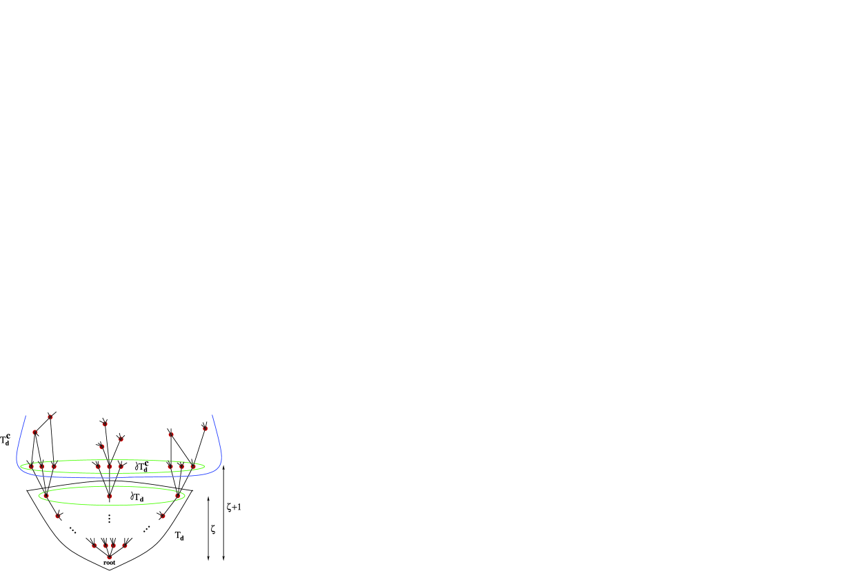
Figure 1: Illustration of $\mathbb{T}_{d}$, $\mathbb{T}_{d}^{c}$, $\partial\mathbb{T}_{d}$ and $\partial\mathbb{T}_{d}^{c}$ starting at a vertex root, with maximal tree depth $\zeta$. Note that the neighbors in $\mathbb{T}_{d}^{c}$ of the vertices from $\partial\mathbb{T}_{d}^{c}$ may, but need not continue the tree-like structure. For this particular tree, $d=4$.

Note that all edges between $\mathbb{T}_{d}$ and $\mathbb{T}_{d}^{c}$ are between $\partial\mathbb{T}_{d}$ and $\partial\mathbb{T}_{d}^{c}$.

Additionally we will denote the set of vertices of $\mathbb{T}_{d}$ (resp., $\mathbb{T}_{d}^{c}$) by $V(\mathbb{T}_{d})$ [resp., $V(\mathbb{T}_{d}^{c})$].

Let $A$ denote the adjacency matrix of this graph, and let $H_{d}$ denote the adjacency matrix of the subgraph $\mathbb{T}_{d}$. Label the vertices of $H_{d}$ as in Lemmas 7 and 8, and write $A$ in the block matrix form

$$A=\left[\matrix{D&B\cr B^{\prime}&H_{d}}\right].$$

Here $D$ is the adjacency matrix of $\mathbb{T}_{d}^{c}$, the matrix $B$ records only and all the edges between $\partial\mathbb{T}_{d}$ and $\partial\mathbb{T}_{d}^{c}$ and we again use the notation $B^{\prime}$ for the transpose of $B$.

We will now proceed to estimate how close the Stieltjes transform of the regular graph is to that of the tree.

Lemma 10

Fix a complex number $z$ such that $z\in E_{r}$ [see (12)] for some $r>1$. Let $\varepsilon$ denote the quantity

$$\varepsilon=\biggl{(}\frac{1}{\sqrt{d-1}}A-z\biggr{)}^{-1}_{\mathrm{root},\mathrm{root}}-\biggl{(}\frac{1}{\sqrt{d-1}}H_{d}-z\biggr{)}^{-1}_{\mathrm{root},\mathrm{root}}.$$

We have the following bound:

$$|\varepsilon|\leq\biggl{(}\frac{2C_{0}^{2}}{1-r^{-2\zeta-4}}\biggr{)}\frac{r^{-2\zeta-2}}{\Im(z)}.$$

Define the vector

$$v=B\biggl{(}\frac{1}{\sqrt{d-1}}H_{d}-z\biggr{)}^{-1}e_{\mathrm{root}},$$

where $e_{\mathrm{root}}$ is the vector that puts mass at the root vertex and zero elsewhere.

Then by using the formula for the inverse of block matrices (18) we get

$$\varepsilon=\frac{1}{d-1}\biggl{\{}v^{\prime}\biggl{(}\frac{1}{\sqrt{d-1}}D-z-\frac{1}{d-1}B\biggl{(}\frac{1}{\sqrt{d-1}}H_{d}-z\biggr{)}^{-1}B^{\prime}\biggr{)}^{-1}v\biggr{\}}.$$ (31)

Our first job is to estimate the elements of the vector $v$. From the definition it is clear that the rows of $B$ (and columns of $B^{\prime}$) are labeled by the vertices of $\mathbb{T}_{d}^{c}$. We write $B_{i*}$ to designate the $i$th row of $B$.

We obtain

$$v_{i} = B_{i*}\biggl{(}\frac{1}{\sqrt{d-1}}H_{d}-z\biggr{)}^{-1}e_{\mathrm{root}}=\sum_{k\in V(\mathbb{T}_{d})}B_{ik}\biggl{(}\frac{1}{\sqrt{d-1}}H_{d}-z\biggr{)}^{-1}_{k,\mathrm{root}}$$

$$= \sum_{k\in V(\mathbb{T}_{d}^{c})}B_{ik}\biggl{(}\frac{1}{\sqrt{d-1}}H_{d}-z\biggr{)}^{-1}_{\mathrm{root},k}\qquad\mbox{by symmetry of $H_{d}$}.$$

Note that $B_{ik}$ is positive (i.e., $1$) if and only if $i\in\partial\mathbb{T}_{d}^{c}$, $k\in\partial\mathbb{T}_{d}$ and $i$ and $k$ have an edge between them. Thus: [(iii)]

$v_{i}=0$ unless $i\in\partial\mathbb{T}^{c}_{d}$.

When $i\in\partial\mathbb{T}_{d}^{c}$,

$$v_{i}=\sum_{k\in\partial\mathbb{T}_{d},k\sim i}\biggl{(}\frac{1}{\sqrt{d-1}}H_{d}-z\biggr{)}^{-1}_{\mathrm{root},k}=\psi_{d}(\zeta).$$ (33)

Here $\psi_{d}(\zeta)$ has been defined in (8). The fact that there is exactly one $k\in\partial\mathbb{T}_{d}$ such that $i\sim k$ follows from our assumption that the $(\zeta+1)$ neighborhood of the root is a tree (see Figure 1).

By counting the number of elements in $\partial\mathbb{T}_{d}^{c}$, we get

$$\|v\|^{2}=d(d-1)^{\zeta}|\psi_{d}(\zeta)|^{2}\leq C_{0}^{2}\frac{dr^{-2\zeta-2}}{1-r^{-2\zeta-4}},$$ (34)

where the final estimate is from (29).

Note that the matrix

$$\biggl{(}\frac{1}{\sqrt{d-1}}D-z-\frac{1}{d-1}B\biggl{(}\frac{1}{\sqrt{d-1}}H_{d}-z\biggr{)}^{-1}B^{\prime}\biggr{)}$$

is precisely the matrix $\mathbb{G}$ appearing in (18). In particular, it is the top left block of the matrix $[(d-1)^{-1/2}A-z]^{-1}$. Hence, by padding the vector $v$ with extra zeros, we get a vector $\bar{v}$ such that

$$\varepsilon=\frac{1}{d-1}\bar{v}^{\prime}\biggl{(}\frac{1}{\sqrt{d-1}}A-z\biggr{)}^{-1}\bar{v}.$$

Since the matrix $A$ is real symmetric, it has only real eigenvalues. It follows from spectral decomposition of the real, symmetric matrix $A$, that for any real vector $y$

$$y^{\prime}\biggl{(}\frac{1}{\sqrt{d-1}}A-z\biggr{)}^{-1}y\leq\frac{\|y\|^{2}}{\Im(z)}.$$ (35)

Observe from (33) that $v=\psi_{d}(\zeta)e$, where $e$ is a real vector of ones and zeroes which is one precisely for the labels corresponding to $\partial\mathbb{T}_{d}$.

Combining our previous observations, we get

$$v^{\prime}\biggl{(}z-\frac{1}{\sqrt{d-1}}D-\frac{1}{d-1}\chi\biggr{)}^{-1}v=\psi_{d}^{2}(\zeta)e^{\prime}\biggl{(}\frac{1}{\sqrt{d-1}}A-z\biggr{)}^{-1}e.$$

Now using the bound from (34) in (31) we get

$$|\varepsilon| \leq \frac{|\psi_{d}^{2}(\zeta)|}{d-1}\frac{\|e\|^{2}}{\Im(z)}=\frac{1}{d-1}\frac{\|v\|^{2}}{\Im(z)}\leq C_{0}^{2}\frac{d}{d-1}\biggl{(}\frac{r^{-2\zeta-2}}{1-r^{-2\zeta-4}}\biggr{)}\frac{1}{\Im(z)}$$

$$\leq \biggl{(}\frac{2C_{0}^{2}}{1-r^{-2\zeta-4}}\biggr{)}\frac{r^{-2\zeta-2}}{\Im(z)}.$$

This completes the proof of the lemma.

We now arrive at our main result about deterministic regular graphs. Consider the set-up as in Lemma 10. Now a consider a sequence of graphs $G_{n}$ such that $G_{n}$ is $d_{n}$-regular. Each $G_{n}$ has a marked vertex called the root such that for some sequence $\{\zeta_{n}\}$, the $\zeta_{n}+1$ neighborhood of the root is acyclic in $G_{n}$.

Lemma 11

Assume that that sequences $\{d_{n}\}$ and $\{\zeta_{n}\}$ both tend to infinity with $n$ with the following restriction. There exists a sequence $r_{n}$ such that

$$r_{n}=e^{d_{n}^{-\alpha}}\qquad\mbox{for some $0<\alpha<1$}\quad\mbox{and}\quad r_{n}^{-\zeta_{n}}=o(1/d_{n}).$$ (36)

Let $U_{n}$ denote all complex numbers $z$ such that $\Im(z)>(r_{n}-r^{1}_{n})/2$. If $A_{n}$ denotes the adjacency matrix of the graph $G_{n}$, for all $d_{n}$ such that $d_{n}\geq(\log 2)^{1/\alpha}$, then for all $z$, eventually in every $U_{n}$, we have

$$\biggl{|}\biggl{(}\frac{1}{\sqrt{d_{n}-1}}A_{n}-z\biggr{)}^{-1}_{\mathrm{root},\mathrm{root}}-s(z)\biggr{|}=O(1/d_{n}),$$ (37)

where $s(z)$ is the Stieltjes transform of the semicircle law $s(z)=-z/2+\sqrt{z^{2}-4}/2$.

Under our assumptions certain simplifications are immediate. The constant $C_{0}$ appearing in Lemma 9 (and later) can be taken to be an absolute constant. Since $r_{n}^{-\zeta_{n}}=o(1/d_{n})$, we can choose $C_{0}$ large enough in (27) such that

$$|\varphi_{d_{n}}(\zeta_{n})-s(z_{n})|\leq C_{0}/d_{n}.$$ (38)

Here $z_{n}$ is any sequence of complex numbers such that $z_{n}/2$ belongs to the ellipse $E_{r_{n}}$ defined in (12).

Note that

$$\varphi_{d_{n}}(\zeta_{n})=\biggl{(}\frac{1}{\sqrt{d_{n}-1}}A_{n}-z_{n}\biggr{)}^{-1}_{\mathrm{root},\mathrm{root}}.$$

We now use Lemma 10.

Consider now

$$\Im(z)\geq\frac{r_{n}-r_{n}^{-1}}{2}=\frac{1}{2}[e^{d_{n}^{-\alpha}}-e^{-d_{n}^{-\alpha}}].$$

One can easily verify the inequality

$$\frac{e^{x}-e^{-x}}{2}\geq x/2\qquad\mbox{for all }x\leq\log 2.$$ (39)

Applying this inequality above, we get $\Im(z)\geq d_{n}^{-\alpha}/2$ for all $d_{n}$ as stated in the lemma.

Combining with Lemma 10 we get

$$|\varepsilon|\leq 2C_{0}^{2}\frac{r_{n}^{-2\zeta_{n}}}{1-r_{n}^{-2\zeta_{n}-4}}d_{n}^{\alpha}\leq C_{1}\frac{1}{d_{n}^{2}}d_{n}^{\alpha}=o(1/d_{n}).$$

Combining with (38) this completes the proof of the theorem.

We will need the following lemma to show that the previous “tree approximation” result about deterministic regular graphs can be applied to the random graph by choosing almost any vertex as the “root.”

Lemma 12

Let $d_{n}=(\log n)^{\gamma}$, for some positive $\gamma$. Let $\{r_{n}\}$ be as in Lemma 11. Let $\eta_{n}$ be defined as $(r_{n}-r_{n}^{-1})/2$. For some $\beta>1$, we define the sequence $\{\zeta_{n},n=1,2,\ldots\}$ satisfying

$$\zeta_{n}=\frac{1}{4}\frac{\log n}{\log(d_{n}-1)}-\beta.$$ (40)

Let $J(n)$ be the set of vertices in $G_{n}$ whose $\zeta_{n}$-neighborhoods are acyclic and let $|J(n)|$ denote its size. Let $\Omega(n)$ be the event

$${|J(n)|}/{n}>1-\eta_{n}/d_{n}.$$ (41)

One can choose $\beta$ no larger than $4$ such that

$$P(\Omega^{c}(n))\leq o\biggl{(}\frac{1}{n}\biggr{)}.$$ (42)

The proof of this result is very similar to the proof of Lemma 4. We again use the estimates of McKay, Wormald and Wysocka mww04 on the Poisson approximation to the number of short cycles. Consider a sequence $\{\zeta_{n}\}$ as in the statement. It is clear from the choice that

$$4\zeta_{n}\log(d_{n}-1)=\log n-\beta\log(d_{n}-1)$$ (43)

or

$$(d_{n}-1)^{4\zeta_{n}}=\frac{n}{(d_{n}-1)^{\beta}}=o(n).$$ (44)

Thus, we can take $g=2\zeta_{n}$ in (6).

The argument is essentially the same as the one used in the proof of Lemma 4; rather than repeating it, we choose to only highlight the differences.

The total number of vertices whose $\zeta_{n}$-neighborhoods are not acyclic can be bounded above by

$$N^{*}_{\zeta_{n}}=\sum_{s=3}^{2\zeta_{n}}s(d_{n}-1)^{(2\zeta_{n}-s)/2}M_{s},$$

where $M_{s}$ is the number of cycles of length $s$.

Taking expectations and variances above we get

$$EN^{*}_{\zeta_{n}}=O\bigl{(}(d_{n}-1)^{2\zeta_{n}}\bigr{)}$$

and

$$\operatorname{Var}(N^{*}_{\zeta_{n}})\leq\zeta_{n}^{2}(2\zeta_{n}+1)(d_{n}-1)^{2\zeta_{n}}+\zeta_{n}^{2}(2\zeta_{n}+d_{n})o(1).$$

We now want to use Chebyshev’s inequality on the quantity $1-|J(n)|/n$.

$$P\biggl{(}1-\frac{|J(n)|}{n}>\frac{\eta_{n}}{d_{n}}\biggr{)} \leq P(N^{*}_{\zeta_{n}}>{n\eta_{n}}/{d_{n}})\leq\frac{d_{n}^{2}}{n^{2}\eta_{n}^{2}}E(N^{*}_{\zeta_{n}})^{2}$$

$$\leq \frac{3d_{n}^{2}\zeta_{n}^{3}(d_{n}-1)^{2\zeta_{n}}}{n^{2}\eta_{n}^{2}}+\frac{3\zeta_{n}^{3}d_{n}^{2}o(1)}{n^{2}\eta_{n}^{2}}$$

$${}+\frac{d_{n}^{2}}{n\eta_{n}^{2}}O\biggl{(}\frac{(d_{n}-1)^{4\zeta_{n}}}{n}\biggr{)}.$$

Let us analyze the three terms that appear above. We use inequality (39) to obtain $\eta_{n}\geq d_{n}^{-\alpha}/2$. Using (43) we get

$$\frac{3d_{n}^{2}\zeta_{n}^{3}(d_{n}-1)^{2\zeta_{n}}}{n^{2}\eta_{n}^{2}} \leq 3d_{n}^{2}\zeta_{n}^{3}\frac{\sqrt{n}}{(d_{n}-1)^{\beta/2}}\frac{1}{n^{2}}4d_{n}^{2\alpha}=\frac{\mathrm{poly}\mbox{-}\mathrm{log}\ n}{n^{3/2}},$$

$$\frac{3\zeta_{n}^{3}d_{n}^{2}o(1)}{n^{2}\eta_{n}^{2}} \leq \frac{12\zeta_{n}^{3}d_{n}^{2+2\alpha}o(1)}{n^{2}}=\frac{\mathrm{poly}\mbox{-}\mathrm{log}\ n}{n^{2}}o(1).$$

The leading term is the last term on the right which is of the order $d_{n}^{2-\beta}/(n\eta_{n}^{2})$, because by (43) we get $(d_{n}-1)^{4\zeta_{n}}/n=(d_{n}-1)^{-\beta}$.

We now choose $\beta>2\alpha+2$ (and thus no larger than $4$, since $\alpha<1$) such that

$$\frac{d_{n}^{2-\beta}}{\eta_{n}^{2}}\leq 4d_{n}^{2-\beta}d_{n}^{2\alpha}=o(1).$$

This completes the proof of the lemma.

3.4 The Stieltjes transform

We bring now all the results of the previous sections together. Below is the first theorem of this section.

Theorem 13

Consider a sequence of $d_{n}$-regular graphs on $n$ vertices where $d_{n}=(\log n)^{\gamma}$ for some $\gamma>0$. Let $A_{n}$ be the adjacency matrix of the graph, and consider the Stieltjes transform

$$s_{n}(z)=\operatorname{tr}\biggl{(}\frac{1}{\sqrt{d_{n}-1}}A_{n}-z\biggr{)}^{-1},\qquad\Im(z)>0.$$

Let $\eta_{n}=(r_{n}-r_{n}^{-1})/2$ where $r_{n}=\exp(d_{n}^{-\alpha})$ for some $0<\alpha<\min(1,1/\gamma)$.

Let $U_{n}$ denote all complex numbers $z$ such that $\Im(z)>\eta_{n}$. Then there is a large enough constant $C>0$ such that the Stieltjes transform of the empirical eigenvalue distribution of the $n\times n$ matrix $A_{n}$ satisfies

$$P\Bigl{(}\sup_{z\in U_{n}}|s_{n}(z)-s(z)|>{C}/{d_{n}}\Bigr{)}\leq o(1/n).$$

Here $s(z)$ refers to the Stieltjes transform of the semicircle law.

We condition on the event $\Omega(n)$ which, from Lemma 12, happens with a probability of at least $1-o(1/n)$.

Consider the set $J(n)$ from the Lemma 12 and write

$$s_{n}(z)=\frac{1}{n}\sum_{k\in J(n)}\biggl{(}\frac{1}{\sqrt{d_{n}-1}}A_{n}-z\biggr{)}^{-1}_{k,k}+\frac{1}{n}\sum_{k\notin J(n)}\biggl{(}\frac{1}{\sqrt{d_{n}-1}}A_{n}-z\biggr{)}^{-1}_{k,k}.$$ (45)

Now, the spectral norm of $(\frac{1}{\sqrt{d_{n}-1}}A_{n}-z)^{-1}$ is bounded above by $1/\Im(z)$, which in turn is bounded above by $\eta_{n}^{-1}$ for all $z\in U_{n}$. Thus, for all $z\in U_{n}$ and all $k$, we have the obvious bound $(\frac{1}{\sqrt{d_{n}-1}}A_{n}-z)^{-1}_{k,k}\leq\eta_{n}^{-1}$.

Summing up over all $k\notin J(n)$, we get

$$\frac{1}{n}\sum_{k\notin J(n)}\biggl{|}\biggl{(}\frac{1}{\sqrt{d_{n}-1}}A_{n}-z\biggr{)}^{-1}_{k,k}\biggr{|}\leq\frac{n-|J(n)|}{n\eta_{n}}\leq\frac{1}{d_{n}},$$

where the final inequality holds on the event $\Omega$. Thus, we get

$$s_{n}(z)=\frac{1}{n}\sum_{k\in J(n)}\biggl{(}\frac{1}{\sqrt{d_{n}-1}}A_{n}-z\biggr{)}^{-1}_{k,k}+O\biggl{(}\frac{1}{d_{n}}\biggr{)}.$$

Now, on the event $\Omega(n)$, every $k\in J(n)$ can be considered as the root for a $d_{n}$-regular tree of depth $\zeta_{n}$. We can now apply Lemmas 10 and 11. Note that, technically, the $\zeta_{n}$ in Lemma 12 and the $\zeta$ used in Lemma 10 differ by at most one; however, this does not affect the following calculations.

We verify the following assumptions from Lemma 11:

$$r_{n}^{-\zeta_{n}} = \exp\biggl{(}-\frac{1}{4}d_{n}^{-\alpha}\frac{\log n}{\log(d_{n}-1)}+\beta d_{n}^{-\alpha}\biggr{)}$$

$$= \exp\biggl{(}-\frac{1}{4}\frac{(\log n)^{1-\alpha\gamma}}{\log(d_{n}-1)}+\frac{\beta}{(\log n)^{\alpha}}\biggr{)}$$

$$\leq C\exp\biggl{(}-\frac{(\log n)^{1-\alpha\gamma}}{4\gamma\log\log n}\biggr{)}\ll\exp(-\gamma\log\log n)=\frac{1}{d_{n}},$$

whenever $\alpha\gamma<1$.

We now combine our error estimate (37) to see that for any $k\in J(n)$, on the event $\Omega(n)$, and for all $z\in U_{n}$, we have

$$\biggl{|}\biggl{(}\frac{1}{\sqrt{d_{n}-1}}A_{n}-z\biggr{)}^{-1}(k,k)-s(z)\biggr{|}=O\biggl{(}\frac{1}{d_{n}}\biggr{)},$$ (46)

where the constants in the $O(\cdot)$ above does not depend on $k$.

Combining this with decomposition (45) we get

$$\sup_{z\in U_{n}}|s_{n}(z)-s(z)|=O\biggl{(}\frac{1}{d_{n}}\biggr{)}$$ (47)

on the event $\Omega(n)$, which holds with probability at least $1-o(1/n)$. This completes the proof of the lemma.

Recall now the setup of Theorem 2. Fix $\delta>0$. Let $d_{n},\eta_{n}$ be as in Theorem 13. Then we will show that there exists an $N$ large enough such that for all $n\geq N$, for any interval $I\subset\mathbb{R}$ of length $|I|\geq\max\{2\eta_{n},\eta_{n}/(-\delta\log\delta)\}$,

$$\biggl{|}\mathcal{N}_{I}-n\int_{I}f_{\mathrm{sc}}(x)\,dx\biggr{|}<\delta n|I|$$

with probability at least $1-o(1/n)$.

Here $\mathcal{N}_{I}$ is the number of eigenvalues of $W_{n}$ in the interval $I$, and $f_{\mathrm{sc}}$ refers to the density of the semicircle law as in (1). Proof of Theorem 2 Theorem 13 leads to Theorem 2 whose proof follows almost identically to Lemma 60 in the article by Tao and Vu taovu . The only major difference between our theorem and Lemma 60 of taovu is the fact that our interval $I$ can lie anywhere on the real line and is not restricted to a subset of $(-2,2)$ as Lemma 60 requires. We provide an outline of the argument but skip the details.

The idea lies in the observation that a good control over the Stieltjes transform near the real line allows one to invert the transform and have an estimate of the empirical spectral density. This is due to the following inversion formula: if $G$ is a continuous distribution on the real line with Stieltjes transform $s_{G}$, one gets

$$G[a,b]=\lim_{\varepsilon\rightarrow 0}\frac{1}{\pi}\int_{a}^{b}\Im\bigl{(}s_{G}(x+i\varepsilon)\bigr{)}\,dx.$$

Fix an interval $I\subseteq[-2,2]$ such that $|I|\geq 2\eta$. Define the function

$$F(y)=\frac{1}{\pi}\int_{I}\frac{\eta_{n}}{\eta_{n}^{2}+(y-x)^{2}}\,dx.$$

Then it follows that if $\lambda_{i}$ denotes the $i$th eigenvalues of the matrix $\frac{1}{\sqrt{d_{n}-1}}A_{n}$, then

$$\frac{1}{n}\sum_{i=1}^{n}F(\lambda_{i}) = \frac{1}{\pi}\int_{I}\frac{1}{n}\sum_{i=1}^{n}\frac{\eta_{n}}{\eta_{n}^{2}+(\lambda_{i}-x)^{2}}\,dx$$

$$= \frac{1}{\pi}\int_{I}\Im\bigl{(}s_{n}(x+i\eta_{n})\bigr{)}\,dx.$$

Also, if $f_{\mathrm{sc}}$ denotes the density of the semicircle law, we get

$$\int_{-2}^{2}F(y)f_{\mathrm{sc}}(y)\,dy=\frac{1}{\pi}\int_{I}\Im\bigl{(}s(x+i\eta_{n})\bigr{)}\,dx.$$

Using the approximation between $s_{n}$ and $s$ obtained in Theorem 13, we get

$$\Biggl{|}\frac{1}{n}\sum_{i=1}^{n}F(\lambda_{i})-\int_{-2}^{2}F(y)f_{\mathrm{sc}}(y)\,dy\Biggr{|} \leq \frac{1}{\pi}\int_{I}|s_{n}(x+i\eta_{n})-s(x+i\eta_{n})|\,dx$$

$$\leq C\frac{|I|}{d_{n}}\qquad\mbox{with probability }1-o\biggl{(}\frac{1}{n}\biggr{)}.$$

Choose $n$ large enough such that $1/d_{n}\leq\delta$ for all subsequent $n$. Thus

$$\frac{1}{n}\sum_{i=1}^{n}F(\lambda_{i})=\int_{-2}^{2}F(y)f_{\mathrm{sc}}(y)\,dy+O(\delta|I|)$$

with probability $1-o({1}/{n})$.

Now following the bounds in taovu , page 60, proof of Lemma 64, we obtain the bounds

$$\int_{-2}^{2}F(y)f_{\mathrm{sc}}(y)\,dy = \int_{I}f_{\mathrm{sc}}\,dy+O\biggl{(}\eta_{n}\log\frac{|I|}{\eta_{n}}\biggr{)},$$

$$\frac{1}{n}\sum_{i=1}^{n}F(\lambda_{i}) = \frac{\mathcal{N}}{n}+O\biggl{(}\eta_{n}\log\frac{|I|}{\eta_{n}}\biggr{)}.$$

Putting all these together we obtain that with probability $1-o(1/n)$, one has

$${\mathcal{N}_{I}}-n\int_{I}f_{\mathrm{sc}}\,dy=O(n\delta|I|)+O\biggl{(}n\eta_{n}\log\frac{|I|}{\eta_{n}}\biggr{)}.$$

Finally, as observed in taovu , the latter term can be absorbed in the former since $|I|\geq\eta_{n}/\delta\log(1/\delta)$. This completes the proof of the theorem.

4 Delocalization of eigenvectors

Closely related to approximation of the empirical spectral distribution is the fact that the $\mathbb{L}^{2}$-norm of a normalized eigenvector restricted to a large subset of the vertices cannot be small. We follow Definition 1 and prove Theorem 1.

Recall the set-up of Theorem 2. Fix $\delta>0$.

Let $T_{n}\subseteq\{1,2,\ldots,n\}$ be a sequence of sets of size $L_{n}=o(\eta_{n}^{-1})$. Let $\Omega_{1}(n)$ be the event that some unit-norm eigenvector of the matrix $A_{n}$ is $(T_{n},\delta)$ localized; that is,

$$\Omega_{1}(n)=\{\exists i\dvtx\|v_{i}|_{T_{n}}\|^{2}\geq 1-\delta\mbox{, for some }v_{i}\mbox{ such that }A_{n}v_{i}=\lambda_{i}v_{i}\}.$$

Then, for all sufficiently large $n$, we will show that

$$P((\Omega_{1}(n))^{c})\geq e^{-L_{n}\eta_{n}/d_{n}}\biggl{(}1-o\biggl{(}\frac{1}{d_{n}}\biggr{)}\biggr{)}=1-o\biggl{(}\frac{1}{d_{n}}\biggr{)}.$$

Proof of Theorem 3 Consider the set $J(n)$, defined in Lemma 12, of vertices whose $\zeta_{n}$-neighborhoods are acyclic. Recall the event $\Omega(n)$, whose probability (as soon as $n$ is large enough) is $1-o(1/n)$, which is that $|J(n)|/n>1-\eta_{n}/d_{n}$.

We first prove part (i). The event $\Omega_{1}(n)$ can be decomposed as two disjoint events depending on whether the set $T_{n}$ is a subset of $J(n)$ or not. We first examine the event

$$\Omega^{\prime}_{1}(n)=\{T_{n}\subseteq J(n)\}\cap\Omega_{1}(n)$$

for purposes of exclusion.

Assume $\omega\in\Omega(n)\cap\Omega^{\prime}_{1}(n)$, and fix $i,v_{i}$ depending on $\omega$ and $n$. The matrix $A_{n}$ has $n$ real eigenvalues and corresponding eigenspaces. The top eigenvalue is $d_{n}$ with corresponding eigenvector $v_{1}=n^{-1/2}\mathbf{1}$, which is completely delocalized. Let us now choose $v_{2},v_{3},\ldots,v_{n}$ to be a set of normalized eigenvectors, corresponding, respectively, to the eigenvalues $\lambda_{2},\lambda_{3},\ldots,\lambda_{n}$ of $\frac{1}{\sqrt{d_{n}-1}}A_{n}$. Fix a subset $T_{n}\subseteq\{1,2,\ldots,n\}$ of size $L_{n}$ as stated in the theorem.

Consider again the Stieltjes transform of the matrix $(d_{n}-1)^{-1/2}A_{n}$ as in the proof of Theorem 13. That is, for $z\in\mathbb{C}$, with $\Im(z)>0$, consider the matrix $(\frac{1}{\sqrt{d_{n}-1}}A_{n}-z)^{-1}$. Then by the spectral representation it follows that for any $1\leq k\leq n$ we get

$$\biggl{(}\frac{1}{\sqrt{d_{n}-1}}A_{n}-z\biggr{)}^{-1}(k,k)=\sum_{j=1}^{n}\frac{v_{j}^{2}(k)}{(\lambda_{j}-z)}.$$

Summing over the vertices $k\in T_{n}$, we get

$$\sum_{k\in T_{n}}\biggl{(}\frac{1}{\sqrt{d_{n}-1}}A_{n}-z\biggr{)}^{-1}(k,k)=\sum_{j=1}^{n}\frac{\sum_{k\in T_{n}}v_{j}^{2}(k)}{(\lambda_{j}-z)}.$$ (48)

Taking the imaginary part on both sides, we get

$$\Im\biggl{(}\sum_{k\in T_{n}}\biggl{(}\frac{1}{\sqrt{d_{n}-1}}A_{n}-z\biggr{)}^{-1}(k,k)\biggr{)} = \sum_{j=1}^{n}\sum_{k\in T_{n}}v_{j}^{2}(k)\Im\biggl{(}\frac{1}{\lambda_{j}-z}\biggr{)}$$

$$\geq \sum_{k\in T_{n}}v_{i}^{2}(k)\Im(\lambda_{i}-z)^{-1}$$

$$\geq (1-\delta)\Im(\lambda_{i}-z)^{-1}.$$

Now we use the fact that for $\omega\in\Omega(n)$ and for all $k\in J(n)$, we get from equation (46) that

$$\sup_{z\in U_{n}}\biggl{|}\biggl{(}\frac{1}{\sqrt{d_{n}-1}}A_{n}-z\biggr{)}^{-1}(k,k)-s(z)\biggr{|}\leq\frac{C}{d_{n}}$$

for some absolute constant $C>0$. Recall that $s(z)$, the Stieltjes transform of the semicircle density, is given by

$$s(z)=\tfrac{1}{2}\bigl{(}-z+\sqrt{z^{2}-4}\bigr{)}.$$

Thus, summing up over all $k$ in $T_{n}$ we get

$$\sup_{z\in S_{n}}\biggl{|}\sum_{k\in T_{n}}\biggl{(}\frac{1}{\sqrt{d_{n}-1}}A_{n}-z\biggr{)}^{-1}(k,k)-L_{n}s(z)\biggr{|}\leq\frac{CL_{n}}{d_{n}}.$$

Combining this estimate with (4) for $z$ such that $\Re(z)=\lambda_{i}$ and $\Im(z)=\eta_{n}$ we get

$$L_{n}\Im(s(z))+CL_{n}/d_{n}\geq\eta_{n}^{-1}(1-\delta)$$

for all $\omega\in\Omega(n)\cap\Omega^{\prime}_{1}(n)$.

Since $\Im(s(z))$ is bounded and $L_{n}=o(\eta_{n}^{-1})$, there is a large enough $N$ such that for all $n\geq N$, this inequality will not hold when $\omega\in\Omega^{\prime}_{1}(n)$. So we get that

$$P\bigl{(}\Omega(n)\cap\Omega_{1}^{\prime}(n)\bigr{)}=0$$ (50)

as soon as $n$ is large enough.

We can now write

$$\Omega_{1}(n)=\bigl{(}(\Omega(n))^{c}\cap\Omega_{1}(n)\bigr{)}\cup\bigl{(}\Omega(n)\cap\Omega_{1}(n)\bigr{)};$$

the probability of the first of the two events above is bounded by the probability of $(\Omega(n))^{c}$ which is $o(1/n)$. Further, by (50), we get that

$$\Omega(n)\cap\Omega_{1}(n)=\Omega(n)\cap\bigl{(}\Omega_{1}(n)\setminus\Omega_{1}^{\prime}(n)\bigr{)}.$$

Note that the last event is equivalent to saying that $\Omega(n)$ and $\Omega_{1}(n)$ happen, and that in addition $T_{n}\not\subseteq J(n)$.

We now bound

$$P\bigl{[}\Omega(n)\cap\bigl{(}\Omega_{1}(n)\setminus\Omega_{1}^{\prime}(n)\bigr{)}\bigr{]} \leq P[\Omega(n)\cap\{T_{n}\not\subseteq J(n)\}]$$

$$= P[\{T_{n}\not\subseteq J(n)\}\mid\Omega(n)]P[\Omega(n)]$$

$$= \biggl{(}1-o\biggl{(}\frac{1}{n}\biggr{)}\biggr{)}P[\{T_{n}\not\subseteq J(n)\}\mid\Omega(n)].$$

Note now that, given the size $j=|J(n)|$, any set of $j$ labels chosen from $\{1,\ldots,n\}$ is just as likely as any other, and independent of the set $T_{n}$. So

$$P[\{T_{n}\not\subseteq J(n)\}\mid|J(n)|=j] = 1-P[\{T_{n}\subseteq J(n)\}\mid|J(n)|=j]$$

$$= 1-\frac{{n-L_{n}\choose j-L_{n}}}{{n\choose j}}$$

$$\leq 1-\frac{(j-L_{n})^{L_{n}}}{n^{L_{n}}}.$$

Since

$$P[\{T_{n}\not\subseteq J(n)\}\mid\Omega(n)]=P\biggl{[}\{T_{n}\not\subseteq J(n)\}\Bigm{|}\frac{|J(n)|}{n}>1-\frac{\eta_{n}}{d_{n}}\biggr{]},$$

it follows from (4) that

$$P[\{T_{n}\not\subseteq J(n)\}\mid\Omega(n)]\leq 1-\biggl{(}1-\frac{\eta_{n}}{d_{n}}-\frac{L_{n}}{n}\biggr{)}^{L_{n}},$$

and since $L_{n}=o(1/\eta_{n})$ and thus $L_{n}/n=o(\eta_{n}/d_{n})$, it follows that

$$P[\{T_{n}\not\subseteq J(n)\}\mid\Omega(n)]\leq 1-e^{-L_{n}\eta_{n}/d_{n}}\biggl{(}1-o\biggl{(}\frac{1}{d_{n}}\biggr{)}\biggr{)}.$$ (52)

Putting all of these together, we conclude that

$$P[\Omega_{1}(n)]\leq 1-e^{-L_{n}\eta_{n}/d_{n}}\biggl{(}1-o\biggl{(}\frac{1}{d_{n}}\biggr{)}\biggr{)},$$

which completes the proof.

Note that part (ii) is proved in (50).

Appendix: Eigenvalues and eigenvectors of regular trees

Our main step in the above proofs was to understand the Stieltjes transforms or the resolvent matrix of a finite tree where every nonleaf vertex has $(d-1)$ children. It is quite straightforward to compute all the eigenvalues of such a tree. Explicit eigenvalues of the tree give us ideas about spacing distribution of eigenvalues of the random regular graph. Fix a positive integer $d\geq 2$.

Lemma 14

Let $\mathbb{T}$ be a finite ordered rooted tree of depth $\zeta\in\mathbb{N}$ such that every vertex has exactly $(d-1)$ children. That is, the root has degree $(d-1)$, and every other vertex, other than the leaves, has degree $d$. Let $H$ denote the adjacency matrix of this graph. [(ii)]

Then, for any complex number $z$ the characteristic polynomial of $H$ is given by

$$\Delta(z;\zeta):=\det\biggl{(}zI-\frac{1}{\sqrt{d-1}}H\biggr{)}=U_{\zeta+1}(z/2)\prod_{i=1}^{\zeta}U_{\zeta+1-i}^{(d-1)^{i}-(d-1)^{i-1}}(z/2).$$

The eigenvalues of the adjacency matrix are given by the following collection. Consider $i=1,2\ldots,\zeta$: then twice the zeros of the Chebyshev polynomial $U_{\zeta+1-i}$ appears with multiplicity $(d-1)^{i}-(d-1)^{i-1}$. For $i=0$, the multiplicity is one.

Recall the recursive labeling of vertices as given in Section 3.2.

To prove conclusion (i), note that when $\zeta=0$ (i.e., the tree has only the root vertex), the equality is trivially true. We proceed by induction. Suppose the equality is true until depth $\zeta-1$. Consider a tree of depth $\zeta$, and label the adjacency $H$ matrix as above. Thus

$$z-\frac{1}{\sqrt{d-1}}H$$

(53)

$$\qquad={{\left[\matrix{z-\dfrac{1}{\sqrt{d-1}}H_{1}&&&&\vspace*{2pt}\cr&z-\dfrac{1}{\sqrt{d-1}}H_{2}&&&-u\vspace*{2pt}\cr&&\cdots&&\vspace*{2pt}\cr&&&z-\dfrac{1}{\sqrt{d-1}}H_{d-1}&\vspace*{2pt}\cr&&-u^{\prime}&&z}\right].}}$$

Here $u$ is the column vector representing the children of the root. Notice that $u$ is $(d-1)^{-1/2}$ exactly at the $(d-1)$ coordinates which are the last elements in each of the block matrices $H_{1},\ldots,H_{d-1}$ and zero elsewhere. The vector $u^{\prime}$ is the transpose of $u$.

We now use the following well-known formula of determinant of block matrices [akin to (16)]:

$$\det\left[\matrix{A&B\cr C&D}\right]=\det(A)\det(D-CA^{-1}B).$$

We apply this to the matrix $z-(d-1)^{-1/2}H$ treating the the final element $[z]$ as one block: note that, by our labeling, in this case $A$ is a diagonal block matrix, and hence its determinant is a product of the determinants of the individual blocks which are all the same and equal to $\Delta(z;\zeta-1)$. Thus we get

$$\Delta(z;\zeta)=\bigl{(}\Delta(z;\zeta-1)\bigr{)}^{d-1}(z-u^{\prime}A^{-1}u).$$

As shown in Section 3.2, the quantity

$$(z-u^{\prime}A^{-1}u) = z+\varphi(\zeta-1)=z-\frac{U_{\zeta-1}(z/2)}{U_{\zeta}(z/2)}$$

$$= \frac{zU_{\zeta}-U_{\zeta-1}}{U_{\zeta}}=\frac{U_{\zeta+1}(z/2)}{U_{\zeta}(z/2)}.$$

Here $U_{n}$ is the Chebyshev polynomial of the second kind. Note the reversal of sign from Section 3.2 which is due to current reversal of sign from the resolvent matrix.

Hence

$$\Delta(z;\zeta)=\frac{U_{\zeta+1}(z/2)}{U_{\zeta}(z/2)}\bigl{(}\Delta(z;\zeta-1)\bigr{)}^{d-1}=\prod_{i=0}^{\zeta}\biggl{[}\frac{U_{\zeta+1-i}(z/2)}{U_{\zeta-i}(z/2)}\biggr{]}^{(d-1)^{i}}.$$

The last term can be verified from the initial conditions of the Chebyshev polynomials.

Simplifying a bit more, we get

$$\Delta(z;\zeta)=U_{\zeta+1}(z/2)\prod_{i=1}^{\zeta}U_{\zeta+1-i}^{(d-1)^{i}-(d-1)^{i-1}}(z/2).$$

For part (ii), note from above that the $i$ many zeroes of $U_{i}$ appear with multiplicity $(d-1)^{i}-(d-1)^{i-1}$. Hence the total number of eigenvalues are

$$\zeta+1+\sum_{i=1}^{\zeta}(\zeta+2-i)[(d-1)^{i}-(d-1)^{i-1}]=\sum_{i=0}^{\zeta}(d-1)^{i},$$

which is the total number of vertices of the tree.

The zeros of Chebyshev polynomials of order $k$ can be easily shown to be given by

$$\cos\biggl{(}\frac{j\pi}{k+1}\biggr{)},\qquad j=1,2,\ldots,k.$$

Thus an interesting phenomenon transpires in this analysis. If we drop the multiplicities and consider the empirical distribution of the distinct eigenvalues, they are the zeros of the Chebyshev polynomials of increasing order. These zeros are cosine transformations of equidistant points on the unit circle; and hence their empirical distribution converges to the arc-sine law. However, the entire empirical spectral distribution converges (see bordlelarge ) to the spectral distribution of the infinite tree which is the semicircle law. The effect of the multiplicities is strong enough to flip the “smile” of the arc-sine law to the “frown” of the semicircle! Also note that the gap of the spectrum from $2$ is about twice of $\pi^{2}/(\zeta+1)^{2}$, and does not depend on $d$.

Some facts about eigenvectors of this tree are also easy to derive and might be also worthwhile to look at. For example, by the spectral theorem, one can write

$$-\frac{U_{\zeta}(z/2)}{U_{\zeta+1}(z/2)}=\varphi(z)=\biggl{(}\frac{1}{\sqrt{d-1}}H-z\biggr{)}^{-1}_{\mathrm{root},\mathrm{root}}=\sum_{i}\frac{\|P_{i}e_{\mathrm{root}}\|^{2}}{\lambda_{i}-z}.$$ (54)

Here the sum on the right goes over distinct eigenvalues of the adjacency matrix and $P_{i}e_{\mathrm{root}}$ refers to the projection of the vector $e_{\mathrm{root}}$ on the eigenspace corresponding to $\lambda_{i}$.

Notice that the above is a meromorphic function of $z$. From the leftmost expression in (54), it is obvious that the function has poles at (twice) the zeros of $U_{\zeta+1}$. It follows then that $P_{i}e_{\mathrm{root}}$ is zero for all eigenvalues except when $\lambda_{i}$ is twice of a root of $U_{\zeta+1}$. However, these roots are simple, as we show in the previous lemma. Hence, $\|P_{i}e_{\mathrm{root}}\|^{2}$ is precise the square of the “root”-coordinate of the $i$th eigenvector.

Its value can be easily computed. For any root $\lambda_{i}$ of $U_{\zeta+1}$, we get

$$\|P_{i}e_{\mathrm{root}}\|^{2}=\lim_{z\rightarrow 2\lambda_{i}}(z-2\lambda_{i})\frac{U_{\zeta}(z/2)}{U_{\zeta+1}(z/2)}=\frac{2U_{\zeta}(\lambda_{i})}{U_{\zeta+1}^{\prime}(\lambda_{i})}.$$

Here $U^{\prime}_{\zeta+1}$ refers to the derivative of the polynomial $U_{\zeta+1}$. Other coordinates can be similarly derived.

References

- (1) {barticle}[mr] \bauthor\bsnmAlon, \bfnmNoga\binitsN., \bauthor\bsnmKrivelevich, \bfnmMichael\binitsM. and \bauthor\bsnmVu, \bfnmVan H.\binitsV. H. (\byear2002). \btitleOn the concentration of eigenvalues of random symmetric matrices. \bjournalIsrael J. Math. \bvolume131 \bpages259–267. \biddoi=10.1007/BF02785860, issn=0021-2172, mr=1942311\endbibitem
- (2) {bbook}[mr] \bauthor\bsnmAnderson, \bfnmGreg W.\binitsG. W., \bauthor\bsnmGuionnet, \bfnmAlice\binitsA. and \bauthor\bsnmZeitouni, \bfnmOfer\binitsO. (\byear2010). \btitleAn Introduction to Random Matrices. \bseriesCambridge Studies in Advanced Mathematics \bvolume118. \bpublisherCambridge Univ. Press, \baddressCambridge. \bidmr=2760897 \bptnotecheck year \endbibitem
- (3) {barticle}[mr] \bauthor\bsnmBai, \bfnmZ. D.\binitsZ. D. (\byear1993). \btitleConvergence rate of expected spectral distributions of large random matrices. I. Wigner matrices. \bjournalAnn. Probab. \bvolume21 \bpages625–648. \bidissn=0091-1798, mr=1217559 \endbibitem
- (4) {barticle}[mr] \bauthor\bsnmBai, \bfnmZ. D.\binitsZ. D., \bauthor\bsnmMiao, \bfnmB. Q.\binitsB. Q. and \bauthor\bsnmPan, \bfnmG. M.\binitsG. M. (\byear2007). \btitleOn asymptotics of eigenvectors of large sample covariance matrix. \bjournalAnn. Probab. \bvolume35 \bpages1532–1572. \biddoi=10.1214/009117906000001079, issn=0091-1798, mr=2330979 \endbibitem
- (5) {bbook}[auto:STB—2011-03-03—12:04:44] \bauthor\bsnmBai, \bfnmZ. D.\binitsZ. D. and \bauthor\bsnmSilverstein, \bfnmJ. W.\binitsJ. W. (\byear2006). \btitleSpectral Analysis of Large Dimensional Random Matrices. \bseriesMathematics Monograph Series \bvolume2. \bpublisherScience Press, \baddressBeijing. \endbibitem
- (6) {barticle}[mr] \bauthor\bsnmBai, \bfnmZ. D.\binitsZ. D. and \bauthor\bsnmYao, \bfnmJ.\binitsJ. (\byear2005). \btitleOn the convergence of the spectral empirical process of Wigner matrices. \bjournalBernoulli \bvolume11 \bpages1059–1092. \biddoi=10.3150/bj/1137421640, issn=1350-7265, mr=2189081 \endbibitem
- (7) {barticle}[mr] \bauthor\bsnmBaik, \bfnmJinho\binitsJ. and \bauthor\bsnmSuidan, \bfnmToufic M.\binitsT. M. (\byear2005). \btitleA GUE central limit theorem and universality of directed first and last passage site percolation. \bjournalInt. Math. Res. Not. IMRN \bvolume6 \bpages325–337. \biddoi=10.1155/IMRN.2005.325, issn=1073-7928, mr=2131383 \endbibitem
- (8) {barticle}[mr] \bauthor\bsnmBaik, \bfnmJinho\binitsJ. and \bauthor\bsnmSuidan, \bfnmToufic M.\binitsT. M. (\byear2007). \btitleRandom matrix central limit theorems for nonintersecting random walks. \bjournalAnn. Probab. \bvolume35 \bpages1807–1834. \biddoi=10.1214/009117906000001105, issn=0091-1798, mr=2349576 \endbibitem
- (9) {barticle}[mr] \bauthor\bsnmBaker, \bfnmT. H.\binitsT. H. and \bauthor\bsnmForrester, \bfnmP. J.\binitsP. J. (\byear1997). \btitleThe Calogero–Sutherland model and generalized classical polynomials. \bjournalComm. Math. Phys. \bvolume188 \bpages175–216. \biddoi=10.1007/s002200050161, issn=0010-3616, mr=1471336 \endbibitem
- (10) {barticle}[mr] \bauthor\bsnmBauer, \bfnmM.\binitsM. and \bauthor\bsnmGolinelli, \bfnmO.\binitsO. (\byear2001). \btitleRandom incidence matrices: Moments of the spectral density. \bjournalJ. Stat. Phys. \bvolume103 \bpages301–337. \biddoi=10.1023/A:1004879905284, issn=0022-4715, mr=1828732 \endbibitem
- (11) {barticle}[mr] \bauthor\bsnmBen Arous, \bfnmG.\binitsG. and \bauthor\bsnmPéché, \bfnmS.\binitsS. (\byear2005). \btitleUniversality of local eigenvalue statistics for some sample covariance matrices. \bjournalComm. Pure Appl. Math. \bvolume58 \bpages1316–1357. \biddoi=10.1002/cpa.20070, issn=0010-3640, mr=2162782 \endbibitem
- (12) {bmisc}[auto:STB—2011-03-03—12:04:44] \bauthor\bsnmBhamidi, \bfnmS.\binitsS., \bauthor\bsnmEvans, \bfnmS.\binitsS. and \bauthor\bsnmSen, \bfnmA.\binitsA. (\byear2008). \bhowpublishedSpectra of random large trees. Preprint. Available at arXiv:0903.3589v2. \endbibitem
- (13) {barticle}[mr] \bauthor\bsnmBordenave, \bfnmCharles\binitsC. and \bauthor\bsnmLelarge, \bfnmMarc\binitsM. (\byear2010). \btitleResolvent of large random graphs. \bjournalRandom Structures Algorithms \bvolume37 \bpages332–352. \biddoi=10.1002/rsa.20313, issn=1042-9832, mr=2724665 \bptnotecheck year \endbibitem
- (14) {bincollection}[auto:STB—2011-03-03—12:04:44] \bauthor\bsnmBrin, \bfnmS.\binitsS. and \bauthor\bsnmLawrence, \bfnmP.\binitsP. (\byear1998). \btitleThe anatomy of a large-scale hypertextual Web search engine. In \bbooktitleProceedings of the Seventh International Conference on World Wide Web 7 \bpages107–117. \bpublisherBrisbane, \baddressAustralia. \endbibitem
- (15) {bincollection}[auto:STB—2011-03-03—12:04:44] \bauthor\bsnmBroder, \bfnmA.\binitsA. and \bauthor\bsnmShamir, \bfnmE.\binitsE. (\byear1987). \btitleOn the second eigenvalue of random regular graphs. In \bbooktitle28th Annual Symposium on Foundations of Computer Science (Los Angeles, 1987) \bpages286–294. \bpublisherIEEE Comput. Soc. Press, \baddressWashington, DC. \endbibitem
- (16) {barticle}[mr] \bauthor\bsnmChatterjee, \bfnmSourav\binitsS. (\byear2006). \btitleA generalization of the Lindeberg principle. \bjournalAnn. Probab. \bvolume34 \bpages2061–2076. \biddoi=10.1214/009117906000000575, issn=0091-1798, mr=2294976 \endbibitem
- (17) {bincollection}[mr] \bauthor\bsnmDeift, \bfnmPercy\binitsP. (\byear2007). \btitleUniversality for mathematical and physical systems. In \bbooktitleInternational Congress of Mathematicians. Vol. I \bpages125–152. \bpublisherEur. Math. Soc., \baddressZürich. \biddoi=10.4171/022-1/7, mr=2334189 \bptnotecheck year \endbibitem
- (18) {barticle}[mr] \bauthor\bsnmDeift, \bfnmPercy\binitsP. and \bauthor\bsnmGioev, \bfnmDimitri\binitsD. (\byear2007). \btitleUniversality at the edge of the spectrum for unitary, orthogonal, and symplectic ensembles of random matrices. \bjournalComm. Pure Appl. Math. \bvolume60 \bpages867–910. \biddoi=10.1002/cpa.20164, issn=0010-3640, mr=2306224 \bptnotecheck year \endbibitem
- (19) {barticle}[auto:STB—2011-03-03—12:04:44] \bauthor\bsnmDekel, \bfnmY.\binitsY., \bauthor\bsnmLee, \bfnmJ. R.\binitsJ. R. and \bauthor\bsnmLinial, \bfnmN.\binitsN. (\byear2011). \btitleEigenvectors of random graphs: Nodal domains. \bjournalRandom Structures Algorithms \bvolume39 \bpages3958. \endbibitem
- (20) {barticle}[mr] \bauthor\bsnmDumitriu, \bfnmIoana\binitsI. and \bauthor\bsnmEdelman, \bfnmAlan\binitsA. (\byear2006). \btitleGlobal spectrum fluctuations for the -Hermite and -Laguerre ensembles via matrix models. \bjournalJ. Math. Phys. \bvolume47 \bpages063302, 36. \biddoi=10.1063/1.2200144, issn=0022-2488, mr=2239975 \endbibitem
- (21) {barticle}[mr] \bauthor\bsnmElon, \bfnmYehonatan\binitsY. (\byear2008). \btitleEigenvectors of the discrete Laplacian on regular graphs—a statistical approach. \bjournalJ. Phys. A \bvolume41 \bpages435203, 17. \biddoi=10.1088/1751-8113/41/43/435203, issn=1751-8113, mr=2453165 \endbibitem
- (22) {bmisc}[auto:STB—2011-03-03—12:04:44] \bauthor\bsnmErdős, \bfnmL.\binitsL., \bauthor\bsnmKnowles, \bfnmA.\binitsA., \bauthor\bsnmYau, \bfnmH. T.\binitsH. T. and \bauthor\bsnmYin, \bfnmJ.\binitsJ. (\byear2011). \bhowpublishedSpectral statistics of Erdős–Rényi graphs I: Local semicircle law. Preprint. http://arxiv.org/abs/ 1103.1919. \endbibitem
- (23) {barticle}[mr] \bauthor\bsnmErdős, \bfnmLászló\binitsL., \bauthor\bsnmPéché, \bfnmSandrine\binitsS., \bauthor\bsnmRamírez, \bfnmJosé A.\binitsJ. A., \bauthor\bsnmSchlein, \bfnmBenjamin\binitsB. and \bauthor\bsnmYau, \bfnmHorng-Tzer\binitsH.-T. (\byear2010). \btitleBulk universality for Wigner matrices. \bjournalComm. Pure Appl. Math. \bvolume63 \bpages895–925. \bidissn=0010-3640, mr=2662426 \endbibitem
- (24) {barticle}[mr] \bauthor\bsnmErdős, \bfnmLászló\binitsL., \bauthor\bsnmRamírez, \bfnmJosé\binitsJ., \bauthor\bsnmSchlein, \bfnmBenjamin\binitsB., \bauthor\bsnmTao, \bfnmTerence\binitsT., \bauthor\bsnmVu, \bfnmVan\binitsV. and \bauthor\bsnmYau, \bfnmHorng-Tzer\binitsH.-T. (\byear2010). \btitleBulk universality for Wigner Hermitian matrices with subexponential decay. \bjournalMath. Res. Lett. \bvolume17 \bpages667–674. \bidissn=1073-2780, mr=2661171 \endbibitem
- (25) {barticle}[mr] \bauthor\bsnmErdős, \bfnmLászló\binitsL., \bauthor\bsnmSchlein, \bfnmBenjamin\binitsB. and \bauthor\bsnmYau, \bfnmHorng-Tzer\binitsH.-T. (\byear2009). \btitleSemicircle law on short scales and delocalization of eigenvectors for Wigner random matrices. \bjournalAnn. Probab. \bvolume37 \bpages815–852. \biddoi=10.1214/08-AOP421, issn=0091-1798, mr=2537522 \endbibitem
- (26) {barticle}[mr] \bauthor\bsnmErdős, \bfnmLászló\binitsL., \bauthor\bsnmSchlein, \bfnmBenjamin\binitsB. and \bauthor\bsnmYau, \bfnmHorng-Tzer\binitsH.-T. (\byear2009). \btitleLocal semicircle law and complete delocalization for Wigner random matrices. \bjournalComm. Math. Phys. \bvolume287 \bpages641–655. \biddoi=10.1007/s00220-008-0636-9, issn=0010-3616, mr=2481753 \endbibitem
- (27) {bmisc}[auto:STB—2011-03-03—12:04:44] \bauthor\bsnmErdős, \bfnmL.\binitsL., \bauthor\bsnmYau, \bfnmH. T.\binitsH. T. and \bauthor\bsnmYin, \bfnmJ.\binitsJ. (\byear2010). \bhowpublishedUniversality for generalized Wigner matrices with Bernoulli distribution. Preprint. Available at arXiv:1003.3813v4. \endbibitem
- (28) {barticle}[mr] \bauthor\bsnmFeige, \bfnmUriel\binitsU. and \bauthor\bsnmOfek, \bfnmEran\binitsE. (\byear2005). \btitleSpectral techniques applied to sparse random graphs. \bjournalRandom Structures Algorithms \bvolume27 \bpages251–275. \biddoi=10.1002/rsa.20089, issn=1042-9832, mr=2155709 \endbibitem
- (29) {barticle}[mr] \bauthor\bsnmFriedman, \bfnmJoel\binitsJ. (\byear1991). \btitleOn the second eigenvalue and random walks in random -regular graphs. \bjournalCombinatorica \bvolume11 \bpages331–362. \biddoi=10.1007/BF01275669, issn=0209-9683, mr=1137767 \endbibitem
- (30) {barticle}[mr] \bauthor\bsnmFriedman, \bfnmJoel\binitsJ. (\byear1993). \btitleSome geometric aspects of graphs and their eigenfunctions. \bjournalDuke Math. J. \bvolume69 \bpages487–525. \biddoi=10.1215/S0012-7094-93-06921-9, issn=0012-7094, mr=1208809 \endbibitem
- (31) {barticle}[mr] \bauthor\bsnmFriedman, \bfnmJoel\binitsJ. (\byear2008). \btitleA proof of Alon’s second eigenvalue conjecture and related problems. \bjournalMem. Amer. Math. Soc. \bvolume195 \bpagesviii+100. \bidissn=0065-9266, mr=2437174 \endbibitem
- (32) {barticle}[mr] \bauthor\bsnmFüredi, \bfnmZ.\binitsZ. and \bauthor\bsnmKomlós, \bfnmJ.\binitsJ. (\byear1981). \btitleThe eigenvalues of random symmetric matrices. \bjournalCombinatorica \bvolume1 \bpages233–241. \biddoi=10.1007/BF02579329, issn=0209-9683, mr=0637828 \endbibitem
- (33) {barticle}[mr] \bauthor\bsnmGuionnet, \bfnmA.\binitsA. and \bauthor\bsnmZeitouni, \bfnmO.\binitsO. (\byear2000). \btitleConcentration of the spectral measure for large matrices. \bjournalElectron. Commun. Probab. \bvolume5 \bpages119–136 (electronic). \bidissn=1083-589X, mr=1781846 \endbibitem
- (34) {bincollection}[mr] \bauthor\bsnmJakobson, \bfnmDmitry\binitsD., \bauthor\bsnmMiller, \bfnmStephen D.\binitsS. D., \bauthor\bsnmRivin, \bfnmIgor\binitsI. and \bauthor\bsnmRudnick, \bfnmZeév\binitsZ. (\byear1999). \btitleEigenvalue spacings for regular graphs. In \bbooktitleEmerging Applications of Number Theory (Minneapolis, MN, 1996). \bseriesIMA Vol. Math. Appl. \bvolume109 \bpages317–327. \bpublisherSpringer, \baddressNew York. \bidmr=1691538 \bptnotecheck year \endbibitem
- (35) {barticle}[mr] \bauthor\bsnmJohansson, \bfnmKurt\binitsK. (\byear1998). \btitleOn fluctuations of eigenvalues of random Hermitian matrices. \bjournalDuke Math. J. \bvolume91 \bpages151–204. \biddoi=10.1215/S0012-7094-98-09108-6, issn=0012-7094, mr=1487983 \endbibitem
- (36) {barticle}[mr] \bauthor\bsnmKesten, \bfnmHarry\binitsH. (\byear1959). \btitleSymmetric random walks on groups. \bjournalTrans. Amer. Math. Soc. \bvolume92 \bpages336–354. \bidissn=0002-9947, mr=0109367 \endbibitem
- (37) {barticle}[mr] \bauthor\bsnmKhorunzhy, \bfnmA.\binitsA. (\byear2001). \btitleSparse random matrices: Spectral edge and statistics of rooted trees. \bjournalAdv. in Appl. Probab. \bvolume33 \bpages124–140. \biddoi=10.1239/aap/999187900, issn=0001-8678, mr=1825319 \endbibitem
- (38) {barticle}[mr] \bauthor\bsnmKhorunzhy, \bfnmAlexei M.\binitsA. M., \bauthor\bsnmKhoruzhenko, \bfnmBoris A.\binitsB. A. and \bauthor\bsnmPastur, \bfnmLeonid A.\binitsL. A. (\byear1996). \btitleAsymptotic properties of large random matrices with independent entries. \bjournalJ. Math. Phys. \bvolume37 \bpages5033–5060. \biddoi=10.1063/1.531589, issn=0022-2488, mr=1411619 \endbibitem
- (39) {barticle}[mr] \bauthor\bsnmKrivelevich, \bfnmMichael\binitsM. and \bauthor\bsnmSudakov, \bfnmBenny\binitsB. (\byear2003). \btitleThe largest eigenvalue of sparse random graphs. \bjournalCombin. Probab. Comput. \bvolume12 \bpages61–72. \biddoi=10.1017/S0963548302005424, issn=0963-5483, mr=1967486 \endbibitem
- (40) {bbook}[mr] \bauthor\bsnmLorentzen, \bfnmLisa\binitsL. and \bauthor\bsnmWaadeland, \bfnmHaakon\binitsH. (\byear2008). \btitleContinued Fractions. Vol. 1. Convergence Theory, \bedition2nd ed. \bseriesAtlantis Studies in Mathematics for Engineering and Science \bvolume1. \bpublisherAtlantis Press, \baddressParis. \bidmr=2433845 \endbibitem
- (41) {barticle}[mr] \bauthor\bsnmLubotzky, \bfnmA.\binitsA., \bauthor\bsnmPhillips, \bfnmR.\binitsR. and \bauthor\bsnmSarnak, \bfnmP.\binitsP. (\byear1988). \btitleRamanujan graphs. \bjournalCombinatorica \bvolume8 \bpages261–277. \biddoi=10.1007/BF02126799, issn=0209-9683, mr=0963118 \endbibitem
- (42) {bbook}[mr] \bauthor\bsnmMason, \bfnmJ. C.\binitsJ. C. and \bauthor\bsnmHandscomb, \bfnmD. C.\binitsD. C. (\byear2003). \btitleChebyshev Polynomials. \bpublisherChapman & Hall/CRC, \baddressBoca Raton, FL. \bidmr=1937591 \endbibitem
- (43) {barticle}[mr] \bauthor\bsnmMcKay, \bfnmBrendan D.\binitsB. D. (\byear1981). \btitleThe expected eigenvalue distribution of a large regular graph. \bjournalLinear Algebra Appl. \bvolume40 \bpages203–216. \biddoi=10.1016/0024-3795(81)90150-6, issn=0024-3795, mr=0629617 \endbibitem
- (44) {barticle}[mr] \bauthor\bsnmMcKay, \bfnmBrendan D.\binitsB. D. and \bauthor\bsnmWormald, \bfnmNicholas C.\binitsN. C. (\byear1997). \btitleThe degree sequence of a random graph. I. The models. \bjournalRandom Structures Algorithms \bvolume11 \bpages97–117. \biddoi=10.1002/(SICI)1098-2418(199709)11:2<97::AID-RSA1>3.3.CO;2-E, issn=1042-9832, mr=1610253 \endbibitem
- (45) {barticle}[mr] \bauthor\bsnmMcKay, \bfnmBrendan D.\binitsB. D., \bauthor\bsnmWormald, \bfnmNicholas C.\binitsN. C. and \bauthor\bsnmWysocka, \bfnmBeata\binitsB. (\byear2004). \btitleShort cycles in random regular graphs. \bjournalElectron. J. Combin. \bvolume11 \bpages12 pp. (electronic). \bidissn=1077-8926, mr=2097332 \endbibitem
- (46) {bbook}[mr] \bauthor\bsnmMehta, \bfnmMadan Lal\binitsM. L. (\byear1991). \btitleRandom Matrices, \bedition2nd ed. \bpublisherAcademic Press, \baddressBoston, MA. \bidmr=1083764 \endbibitem
- (47) {bincollection}[auto:STB—2011-03-03—12:04:44] \bauthor\bsnmMeila, \bfnmM.\binitsM. and \bauthor\bsnmShi, \bfnmJ.\binitsJ. (\byear2011). \btitleLearning segmentation with random walks. In \bbooktitleAdv. Neural Inf. Process. Syst. \bvolume14 \bpages873–879. \bpublisherMIT Press, \baddressCambridge, MA. \endbibitem
- (48) {barticle}[mr] \bauthor\bsnmMirlin, \bfnmA. D.\binitsA. D. and \bauthor\bsnmFyodorov, \bfnmYan V.\binitsY. V. (\byear1991). \btitleUniversality of level correlation function of sparse random matrices. \bjournalJ. Phys. A \bvolume24 \bpages2273–2286. \bidissn=0305-4470, mr=1118532 \endbibitem
- (49) {barticle}[mr] \bauthor\bsnmMorgenstern, \bfnmMoshe\binitsM. (\byear1994). \btitleExistence and explicit constructions of regular Ramanujan graphs for every prime power . \bjournalJ. Combin. Theory Ser. B \bvolume62 \bpages44–62. \biddoi=10.1006/jctb.1994.1054, issn=0095-8956, mr=1290630 \endbibitem
- (50) {bbook}[mr] \bauthor\bsnmMuirhead, \bfnmRobb J.\binitsR. J. (\byear1982). \btitleAspects of Multivariate Statistical Theory. \bpublisherWiley, \baddressNew York. \bidmr=0652932 \endbibitem
- (51) {barticle}[mr] \bauthor\bsnmPothen, \bfnmAlex\binitsA., \bauthor\bsnmSimon, \bfnmHorst D.\binitsH. D. and \bauthor\bsnmLiou, \bfnmKang-Pu\binitsK.-P. (\byear1990). \btitlePartitioning sparse matrices with eigenvectors of graphs. \bjournalSIAM J. Matrix Anal. Appl. \bvolume11 \bpages430–452. \biddoi=10.1137/0611030, issn=0895-4798, mr=1054210 \endbibitem
- (52) {barticle}[mr] \bauthor\bsnmSemerjian, \bfnmGuilhem\binitsG. and \bauthor\bsnmCugliandolo, \bfnmLeticia F.\binitsL. F. (\byear2002). \btitleSparse random matrices: The eigenvalue spectrum revisited. \bjournalJ. Phys. A \bvolume35 \bpages4837–4851. \biddoi=10.1088/0305-4470/35/23/303, issn=0305-4470, mr=1916090 \endbibitem
- (53) {barticle}[auto:STB—2011-03-03—12:04:44] \bauthor\bsnmShi, \bfnmJ.\binitsJ. and \bauthor\bsnmMalik, \bfnmJ.\binitsJ. (\byear2000). \btitleNormalized cuts and image segmentation. \bjournalIEEE Transactions on Pattern Analysis and Machine Intelligence \bvolume22 \bpages888–905. \endbibitem
- (54) {barticle}[mr] \bauthor\bsnmSoshnikov, \bfnmAlexander\binitsA. (\byear1999). \btitleUniversality at the edge of the spectrum in Wigner random matrices. \bjournalComm. Math. Phys. \bvolume207 \bpages697–733. \biddoi=10.1007/s002200050743, issn=0010-3616, mr=1727234 \endbibitem
- (55) {barticle}[mr] \bauthor\bsnmTao, \bfnmTerence\binitsT. and \bauthor\bsnmVu, \bfnmVan\binitsV. (\byear2010). \btitleRandom matrices: Universality of local eigenvalue statistics up to the edge. \bjournalComm. Math. Phys. \bvolume298 \bpages549–572. \biddoi=10.1007/s00220-010-1044-5, issn=0010-3616, mr=2669449 \bptnotecheck year \endbibitem
- (56) {bmisc}[auto:STB—2011-03-03—12:04:44] \bauthor\bsnmTao, \bfnmT.\binitsT. and \bauthor\bsnmVu, \bfnmV.\binitsV. (\byear2011). \bhowpublishedRandom matrices: Universality of local eigenvalue statistics. Acta Math. To appear. Available at arXiv:0906.0510v10. \endbibitem
- (57) {bincollection}[mr] \bauthor\bsnmTracy, \bfnmCraig A.\binitsC. A. and \bauthor\bsnmWidom, \bfnmHarold\binitsH. (\byear1999). \btitleUniversality of the distribution functions of random matrix theory. In \bbooktitleStatistical Physics on the Eve of the 21st Century. \bseriesSeries on Advances in Statistical Mechanics \bvolume14 \bpages230–239. \bpublisherWorld Sci. Publishing, \baddressRiver Edge, NJ. \bidmr=1704004 \endbibitem
- (58) {bincollection}[mr] \bauthor\bsnmTracy, \bfnmCraig A.\binitsC. A. and \bauthor\bsnmWidom, \bfnmHarold\binitsH. (\byear2000). \btitleUniversality of the distribution functions of random matrix theory. In \bbooktitleIntegrable Systems: From Classical to Quantum (Montréal, QC, 1999). \bseriesCRM Proceedings & Lecture Notes \bvolume26 \bpages251–264. \bpublisherAmer. Math. Soc., \baddressProvidence, RI. \bidmr=1791893 \endbibitem
- (59) {bincollection}[mr] \bauthor\bsnmTracy, \bfnmC. A.\binitsC. A. and \bauthor\bsnmWidom, \bfnmH.\binitsH. (\byear2000). \btitleThe distribution of the largest eigenvalue in the Gaussian ensembles. In \bbooktitleCalogero–Moser–Sutherland Models (\beditor\bfnmJ. F.\binitsJ. F. \bsnmvanDiejen and \beditor\bfnmL.\binitsL. \bsnmVinet, eds.). \bseriesCRM Series in Mathematical Physics \bvolume4 \bpages461–472. \bpublisherSpringer, \baddressNew York. \endbibitem
- (60) {bmisc}[mr] \bauthor\bsnmTran, \bfnmL.\binitsL., \bauthor\bsnmVu, \bfnmVan\binitsV. and \bauthor\bsnmWang, \bfnmK.\binitsK. (\byear2010). \bhowpublishedSparse random graphs: Eigenvalues and eigenvectors. Preprint. Available at http://www.math.rutgers.edu/ ~linhtran/. \endbibitem
- (61) {bincollection}[auto:STB—2011-03-03—12:04:44] \bauthor\bsnmWeiss, \bfnmY.\binitsY. (\byear1999). \btitleSegmentation using eigenvectors: A unifying view. In \bbooktitleProc. of the 7th IEEE Intern. Conf. on Computer Vision, Vol. 2 \bpages975–982. \bpublisherIEEE Press, \baddressNew York. \endbibitem